Sklar’s theorem in an imprecise setting

Abstract.

Sklar’s theorem is an important tool that connects bidimensional distribution functions with their marginals by means of a copula. When there is imprecision about the marginals, we can model the available information by means of p-boxes, that are pairs of ordered distribution functions. Similarly, we can consider a set of copulas instead of a single one. We study the extension of Sklar’s theorem under these conditions, and link the obtained results to stochastic ordering with imprecision.

Keywords. Sklar’s theorem, copula, p-boxes, natural extension, independent products, stochastic orders.

1. Introduction

In this paper, we deal with the problem of combining two marginal models representing the probabilistic information about two random variables $X,Y$ into a bivariate model of the joint behaviour of $(X,Y)$. In the classical case, this problem has a simple solution, by means of Sklar’s well-known theorem [26], that tells us that any bivariate distribution function can be obtained as the combination of its marginals by means of a copula [19].

Here we investigate to what extent Sklar’s theorem can be extended in the context of imprecision, both in the marginal distribution functions and in the copula that links them. The imprecision in marginal distributions shall be modelled by a probability box [10] (p-box, for short), that summarizes a set of distribution functions by means of its lower and upper envelopes. Regarding the imprecision about the copula, we shall also consider a set of copulas. This set shall be represented by means of the newly introduced notion of imprecise copula, that we study in Section 3.1. This imprecision means that in the bivariate case we end up with a set of bivariate distribution functions, that we can summarize by means of a coherent bivariate p-box, a notion recently studied in [22].

Interestingly, we shall show in Section 3.1 that Sklar’s theorem can be only partly extended to the imprecise case; although the combination of two marginal p-boxes by means of a set of copulas (or its associated imprecise copula) always produces a coherent bivariate p-box, the most important aspect of the theorem does not hold: not every coherent bivariate p-box can be obtained in this manner. In Sections 3.2 and 3.3, we consider two particular cases of interest: that where we have no information about the copula that links the two variables together, and that where we assume that the two variables are independent. In those cases, we use Walley’s notions of natural extension [28] and (epistemic) independent products [4, 28] to derive the joint model.

In Section 4, we connect our results to decision making by applying the notion of stochastic dominance in this setting, and we establish a number of cases in which the order existing on the marginals is preserved by their respective joints. We conclude the paper with some additional comments and remarks in Section 5.

2. Preliminary concepts

2.1. Coherent lower previsions

Let us introduce the basic notions from the theory of coherent lower previsions that we shall use later on in this paper. For a more detailed exposition of the theory and for a behavioural interpretation of the concepts below in terms of betting rates, we refer to [28].

Let $\Omega$ be a possibility space. A gamble is a bounded real-valued function $f:\Omega\rightarrow\mathbb{R}$. We shall denote by $\mathcal{L}(\Omega)$ the set of all gambles on $\Omega$, and by $\mathcal{L}^{+}(\Omega)$ the set of non-negative gambles. It includes in particular the indicator functions of subsets $B$ of $\Omega$, i.e., the gambles that take value $1$ on the elements of $B$ and $0$ elsewhere. In this paper, we shall use the same symbol for an event $B$ and for its indicator function.

A lower prevision is a functional $\underline{P}:\mathcal{K}\rightarrow\mathbb{R}$ defined on some set of gambles $\mathcal{K}\subseteq\mathcal{L}(\Omega)$. Here we are interested in lower previsions satisfying the property of coherence:

Definition 1 (Coherent lower previsions).

A lower prevision $\underline{P}:\mathcal{L}(\Omega)\rightarrow\mathbb{R}$ is called coherent when it satisfies the following conditions for every pair of gambles $f,g\in\mathcal{L}(\Omega)$ and every $\lambda>0$:

• $\underline{P}(f)\geq\inf_{\omega\in\Omega}f(\omega)$.

• $\underline{P}(\lambda f)=\lambda\underline{P}(f)$.

• $\underline{P}(f+g)\geq\underline{P}(f)+\underline{P}(g)$.

The restriction to events of a coherent lower prevision is called a coherent lower probability, and more generally a lower prevision $\underline{P}$ on $\mathcal{K}$ is said to be coherent whenever it can be extended to a coherent lower prevision on $\mathcal{L}(\Omega)$. On the other hand, if $\underline{P}$ is a coherent lower prevision on $\mathcal{L}(\Omega)$ and it satisfies (C3) with equality for every $f$ and $g$ in $\mathcal{L}(\Omega)$, then it is called a linear prevision, and its restriction to events is a finitely additive probability. In fact, coherent lower previsions can be given the following sensitivity analysis interpretation: a lower prevision $\underline{P}$ on $\mathcal{K}$ is coherent if and only if it is the lower envelope of its associated credal set,

(1) $$\mathcal{M}(\underline{P}):=\{P:\mathcal{L}(\Omega)\rightarrow\mathbb{R}\text{ linear prevision}:P(f)\geq\underline{P}(f)\ \forall f\in\mathcal{K}\},$$

and as a consequence the lower envelope of a set of linear previsions is always a coherent lower prevision [28, Section 3.3.3(b)].

One particular instance of coherent lower probabilities are those associated with $p$-boxes.

Definition 2.

[10] A (univariate) $p$-box is a pair $(\underline{F},\overline{F})$ where $\underline{F},\overline{F}:\overline{\mathbb{R}}\rightarrow[0,1]$ are cumulative distribution functions (i.e., monotone and such that $\underline{F}(-\infty)=\overline{F}(-\infty)=0,\underline{F}(+\infty)=\overline{F}(+\infty)=1$) satisfying $\underline{F}(x)\leq\overline{F}(x)$ for every $x\in\overline{\mathbb{R}}$.

Define the set $A_{x}=[-\infty,x]$ for every $x\in\overline{\mathbb{R}}$, and let

$$\mathcal{E}_{0}:=\{A_{x}:x\in\overline{\mathbb{R}}\}\cup\{A_{x}^{c}:x\in\overline{\mathbb{R}}\}.$$

Then [27] a $p$-box $(\underline{F},\overline{F})$ induces a coherent lower probability $\underline{P}_{(\underline{F},\overline{F})}:\mathcal{E}_{0}\rightarrow[0,1]$ by

(2) $$\underline{P}_{(\underline{F},\overline{F})}(A_{x})=\underline{F}(x)\text{ and }\underline{P}_{(\underline{F},\overline{F})}(A_{x}^{c})=1-\overline{F}(x)\ \forall x\in\overline{\mathbb{R}}.$$

2.2. Bivariate $p$-boxes

In [22], the notion of $p$-box from Definition 2 has been extended to the bivariate case, to describe couples of random variables $(X,Y)$ in presence of imprecision.

Definition 3.

[22] A map $F:\overline{\mathbb{R}}\times\overline{\mathbb{R}}\rightarrow[0,1]$ is called standardized when it is component-wise increasing, that is, $F(t_{1},z)\leq F(t_{2},z)$ and $F(z,t_{1})\leq F(z,t_{2})$ for all $t_{1}\leq t_{2}$ and $z$, and satisfies

$$F(-\infty,y)=F(x,-\infty)=0\ \forall x,y\in\overline{\mathbb{R}},\ F(+\infty,+\infty)=1.$$

It is called a distribution function for $(X,Y)$ when it is standardized and satisfies

$$F(x_{2},y_{2})+F(x_{1},y_{1})-F(x_{1},y_{2})-F(x_{2},y_{1})\geq 0$$

for all $x_{1},x_{2},y_{1},y_{2}\in\overline{\mathbb{R}}$ such that $x_{1}\leq x_{2}$, $y_{1}\leq y_{2}$ (with equality holding whenever $(x_{1}\leq X<x_{2})\wedge(y_{1}\leq Y<y_{2})$ is impossible). Given two standardized functions $\underline{F},\overline{F}:\overline{\mathbb{R}}\times\overline{\mathbb{R}}\rightarrow[0,1]$ satisfying $\underline{F}(x,y)\leq\overline{F}(x,y)$ for every $x,y\in\overline{\mathbb{R}}$, the pair $(\underline{F},\overline{F})$ is called a bivariate $p$-box.

Bivariate $p$-boxes are introduced as a model for the imprecise knowledge of a bivariate distribution function. The reason why the lower and upper functions in a bivariate $p$-box are not required to be distribution functions is that the lower and upper envelopes of a set of bivariate distribution functions need not be distribution functions themselves, as showed in [22].

Let $(\underline{F},\overline{F})$ be a bivariate $p$-box on $\overline{\mathbb{R}}\times\overline{\mathbb{R}}$. Define $A_{(x,y)}=[-\infty,x]\times[-\infty,y]$ for every $x,y\in\overline{\mathbb{R}}$, and consider the sets

$${\mathcal{D}}:=\{A_{(x,y)}:x,y\in\overline{\mathbb{R}}\},{\mathcal{D}}_{c}:=\{A_{(x,y)}^{c}:x,y\in\overline{\mathbb{R}}\},\ \mathcal{E}:={\mathcal{D}}\cup{\mathcal{D}}_{c}.$$

Note that $A_{(+\infty,+\infty)}=\overline{\mathbb{R}}\times\overline{\mathbb{R}}$, whence both $\overline{\mathbb{R}}\times\overline{\mathbb{R}}$ and $\emptyset$ belong to ${\mathcal{E}}$. Similarly to Eq. (2), we can define the lower probability induced by a bivariate $p$-box $(\underline{F},\overline{F})$ on $\overline{\mathbb{R}}\times\overline{\mathbb{R}}$ as the map $\underline{P}_{(\underline{F},\overline{F})}:{\mathcal{E}}\rightarrow[0,1]$ given by:

(3) $$\underline{P}_{(\underline{F},\overline{F})}(A_{(x,y)})=\underline{F}(x,y),\ \ \underline{P}_{(\underline{F},\overline{F})}(A_{(x,y)}^{c})=1-\overline{F}(x,y)$$

for every $x,y\in\overline{\mathbb{R}}$. Conversely, a lower probability $\underline{P}:\mathcal{E}\rightarrow[0,1]$ determines a couple of functions $\underline{F}_{\underline{P}},\overline{F}_{\underline{P}}:\overline{\mathbb{R}}\times\overline{\mathbb{R}}\rightarrow[0,1]$ defined by

(4) $$\underline{F}_{\underline{P}}(x,y)=\underline{P}(A_{(x,y)})\text{ and }\overline{F}_{\underline{P}}(x,y)=1-\underline{P}(A_{(x,y)}^{c})\ \forall x,y\in\overline{\mathbb{R}}.$$

Then $(\underline{F}_{\underline{P}},\overline{F}_{\underline{P}})$ is a bivariate $p$-box as soon as the lower probability $\underline{P}$ is $2$-coherent [22]. $2$-coherence is a weak rationality condition implied by coherence [28, Appendix B], which in the context of this paper, where the domain $\mathcal{E}$ is closed under complementation, is equivalent [22] to $\underline{P}_{(\underline{F},\overline{F})}$ being monotone, normalised, and such that $\underline{P}_{(\underline{F},\overline{F})}(E)+\underline{P}_{(\underline{F},\overline{F})}(E^{c})\leq 1$ for every $E\in{\mathcal{E}}$.

The correspondence between bivariate $p$-boxes and lower probabilities in terms of precise models is given by the following lemma:

Lemma 1.

[22] Let $(\underline{F},\overline{F})$ be a $p$-box and $\underline{P}_{(\underline{F},\overline{F})}$ the lower probability it induces on $\mathcal{E}$ by means of Eq. (3).

• Let $P$ be (the restriction to $\mathcal{E}$ of) a linear prevision on $\mathcal{L}(\overline{\mathbb{R}}\times\overline{\mathbb{R}})$, and let $F_{P}$ be its associated distribution function given by $F_{P}(x,y)=P(A_{(x,y)})$ for every $x,y\in\overline{\mathbb{R}}$. Then

  $$P(A)\geq\underline{P}_{(\underline{F},\overline{F})}(A)\ \forall A\in{\mathcal{E}}\iff\underline{F}\leq F_{P}\leq\overline{F}.$$

• Conversely, let $F$ be a distribution function on $\overline{\mathbb{R}}\times\overline{\mathbb{R}}$, and let $P_{F}:{\mathcal{E}}\rightarrow[0,1]$ be the functional given by $P_{F}(A_{(x,y)})=F(x,y),P_{F}(A_{(x,y)}^{c})=1-F(x,y)$ for every $x,y\in\overline{\mathbb{R}}$. Then

  $$\underline{F}\leq F\leq\overline{F}\iff P_{F}(A)\geq\underline{P}_{(\underline{F},\overline{F})}(A)\ \forall A\in{\mathcal{E}}.$$

Given a bivariate $p$-box $(\underline{F},\overline{F})$, Lemma 1 implies that the coherence of its associated lower probability $\underline{P}_{(\underline{F},\overline{F})}$ can be characterised through a set of distribution functions:

Proposition 1.

[22] The lower probability $\underline{P}_{(\underline{F},\overline{F})}$ induced by the bivariate $p$-box $(\underline{F},\overline{F})$ by means of Eq. (3) is coherent if and only if $\underline{F}$ (resp., $\overline{F}$) is the lower (resp., upper) envelope of the set

(5) $${\mathcal{F}}=\{F:\overline{\mathbb{R}}\times\overline{\mathbb{R}}\rightarrow[0,1]\text{ distribution function}:\underline{F}\leq F\leq\overline{F}\}.$$

If $\underline{P}_{(\underline{F},\overline{F})}$ is coherent, the following conditions hold for every $x_{1}\leq x_{2}\in\overline{\mathbb{R}}$ and $y_{1}\leq y_{2}\in\overline{\mathbb{R}}$:

(I-RI1) $$\underline{F}(x_{2},y_{2})+\overline{F}(x_{1},y_{1})-\underline{F}(x_{1},y_{2})-\underline{F}(x_{2},y_{1})\geq 0.$$

(I-RI2) $$\overline{F}(x_{2},y_{2})+\underline{F}(x_{1},y_{1})-\underline{F}(x_{1},y_{2})-\underline{F}(x_{2},y_{1})\geq 0.$$

(I-RI3) $$\overline{F}(x_{2},y_{2})+\overline{F}(x_{1},y_{1})-\overline{F}(x_{1},y_{2})-\underline{F}(x_{2},y_{1})\geq 0.$$

(I-RI4) $$\overline{F}(x_{2},y_{2})+\overline{F}(x_{1},y_{1})-\underline{F}(x_{1},y_{2})-\overline{F}(x_{2},y_{1})\geq 0.$$

Definition 4.

A bivariate $p$-box $(\underline{F},\overline{F})$ is coherent whenever the lower probability $\underline{P}_{(\underline{F},\overline{F})}$ it induces on $\mathcal{E}$ by means of Eq. (3) is coherent.

2.3. Copulas

In this paper, we are going to study to what extent bivariate $p$-boxes can be expressed as a function of their marginals. In the precise case (that is, when we have only one bivariate distribution function), this is done through the notion of copula.

Definition 5.

[19] A function $C:[0,1]\times[0,1]\rightarrow[0,1]$ is called a copula when it satisfies the following conditions:

(COP1) $$C(0,u)=C(u,0)=0\ \forall u\in[0,1].$$

(COP2) $$C(1,u)=C(u,1)=u\ \forall u\in[0,1].$$

(COP3) $$C(u_{2},v_{2})+C(u_{1},v_{1})-C(u_{1},v_{2})-C(u_{2},v_{1})\geq 0\ \forall u_{1}\leq u_{2},v_{1}\leq v_{2}\in[0,1].$$

It follows from the definition above that a copula is component-wise monotone increasing. One of the main features of copulas lies in Sklar’s theorem:

Theorem 1 ([26], Sklar’s Theorem).

Let $F_{\rm(X,Y)}:\overline{\mathbb{R}}\times\overline{\mathbb{R}}\rightarrow[0,1]$ be a bivariate distribution function with marginals $F_{\rm X}:\overline{\mathbb{R}}\rightarrow[0,1]$ and $F_{\rm Y}:\overline{\mathbb{R}}\rightarrow[0,1]$, defined by $F_{\rm X}(x)=F_{\rm(X,Y)}(x,+\infty)$ and $F_{\rm Y}(y)=F_{\rm(X,Y)}(+\infty,y)$ for any $x$ and $y$ in $\overline{\mathbb{R}}$. Then there is a copula $C$ such that

$$F_{\rm(X,Y)}(x,y)=C(F_{\rm X}(x),F_{\rm Y}(y))\mbox{ for all }(x,y)\in\overline{\mathbb{R}}\times\overline{\mathbb{R}}.$$

Conversely, any transformation of marginal distribution functions by means of a copula produces a bivariate distribution function.

Any copula $C$ must satisfy the Fréchet-Hoeffding bounds (see [11, 29]):

(6) $$C_{\rm L}(u,v):=\max\{u+v-1,0\}\leq C(u,v)\leq\min\{u,v\}:=C_{\rm M}(u,v)$$

for every $u,v\in[0,1]$. $C_{\rm L}$ is called the Łukasiewicz copula and $C_{\rm M}$ the minimum copula. Eq. (6) applies in particular to one instance of copulas that shall be of interest in this paper: the product copula $C_{\rm P}$, given by $C_{\rm P}(u,v)=u\cdot v$ for every $u,v\in[0,1]$. It holds that two random variables $X,Y$ are stochastically independent if and only if their distribution functions are coupled by the product copula.

For an in-depth review on copulas we refer to [19].

3. Combining marginal $p$-boxes into a bivariate one

One particular context where bivariate $p$-boxes can arise is in the joint extension of two marginal $p$-boxes. In this section, we explore this case in detail, studying in particular the properties of some bivariate $p$-boxes with given marginals: the largest one, that shall be obtained by means of the Fréchet bounds and the notion of natural extension, and the one modelling the notion of independence. In both cases, we shall see that the bivariate model can be derived by means of an appropriate extension of the notion of copula.

Related results can be found in [27, Section 7], with one fundamental difference: in [27], the authors use the existence of a total preorder on the product space (in the case of this paper, $\overline{\mathbb{R}}\times\overline{\mathbb{R}}$) that is compatible with the orders in the marginal spaces, and reduce the multivariate p-box to a univariate one. Here we do no such reduction, and we consider only a partial order: the product order, given by

$$(x_{1},y_{1})\leq(x_{2},y_{2})\Leftrightarrow x_{1}\leq x_{2}\text{ and }y_{1}\leq y_{2}.$$

Another related study was made by Yager in [30], considering the case in which the marginal distributions are not precisely described and are defined by means of Dempster-Shafer belief structures instead. He modelled this situation by considering copulas whose arguments are intervals (the ones determined by the Demspter-Shafer models) instead of crisp numbers, and whose images are also intervals. He showed then that the lower (resp., upper) bound of the interval of images corresponds to the copula evaluated in the lower (resp., upper) bounds of the intervals. This can be seen as a particular case of our subsequent Proposition 4.

3.1. A generalization of Sklar’s theorem

Let us study to which extent Sklar’s theorem can be generalised to a context of imprecision, both in the marginal distribution functions to be combined and in the copula that links them. In order to tackle this problem, we introduce the notion of imprecise copula:

Definition 6.

A pair $(\underline{C},\overline{C})$ of functions $\underline{C},\overline{C}:[0,1]\times[0,1]\rightarrow[0,1]$ is called an imprecise copula if:

• $\underline{C}(0,u)=\underline{C}(u,0)=0$, $\underline{C}(1,u)=\underline{C}(u,1)=u$ $\forall u\in[0,1]$.

• $\overline{C}(0,u)=\overline{C}(u,0)=0$, $\overline{C}(1,u)=\overline{C}(u,1)=u$ $\forall u\in[0,1]$.

• For any $u_{1}\leq u_{2},v_{1}\leq v_{2}$:

  (CI-1) $${}\underline{C}(u_{2},v_{2})+\overline{C}(u_{1},v_{1})-\underline{C}(u_{1},v_{2})-\underline{C}(u_{2},v_{1})\geq 0.$$

  (CI-2) $$\overline{C}(u_{2},v_{2})+\underline{C}(u_{1},v_{1})-\underline{C}(u_{1},v_{2})-\underline{C}(u_{2},v_{1})\geq 0.$$

  (CI-3) $$\overline{C}(u_{2},v_{2})+\overline{C}(u_{1},v_{1})-\overline{C}(u_{1},v_{2})-\underline{C}(u_{2},v_{1})\geq 0.$$

  (CI-4) $$\overline{C}(u_{2},v_{2})+\overline{C}(u_{1},v_{1})-\underline{C}(u_{1},v_{2})-\overline{C}(u_{2},v_{1})\geq 0.$$

We are using the terminology imprecise copula in the definition above because we intend it as a mathematical model for the imprecise knowledge of a copula; note however that the lower and upper functions $\underline{C},\overline{C}$ need not be copulas themselves, because they may not satisfy the 2-increasing property (COP3).

(CI-1)$\div$(CI-4) are useful in establishing the following properties of imprecise copulas.

Proposition 2.

Let $(\underline{C},\overline{C})$ be an imprecise copula.

• $\underline{C}\leq\overline{C}$.

• $\underline{C}$ and $\overline{C}$ are component-wise increasing.

• The Lipschitz condition

  (7) $$|C(u_{2},v_{2})-C(u_{1},v_{1})|\leq|u_{2}-u_{1}|+|v_{2}-v_{1}|\ \forall u_{1},u_{2},v_{1},v_{2}\in[0,1]$$

  is satisfied both by $C=\underline{C}$ and by $C=\overline{C}$.

• The pointwise infimum and supremum of a non-empty set of copulas $\mathcal{C}$ form an imprecise copula.

Proof.

• This follows from inequality (CI-3), with $u_{2}=u_{1}$.

• Use (CI-1) with, alternatively, $v_{1}=0$ and $u_{1}=0$ to obtain, respectively,

  $$\underline{C}(u_{2},v_{2})-\underline{C}(u_{1},v_{2})\geq 0 \ \forall v_{2},u_{1},u_{2}\in[0,1],s.t.\ u_{1}\leq u_{2}$$

  $$\underline{C}(u_{2},v_{2})-\underline{C}(u_{2},v_{1})\geq 0 \ \forall u_{2},v_{1},v_{2}\in[0,1],s.t.\ v_{1}\leq v_{2}$$

  By these inequalities, $\underline{C}$ is component-wise increasing. Analogously, to prove that $\overline{C}$ is component-wise increasing, apply (CI-4) with $u_{1}=0$ and (CI-3) with $v_{1}=0$.

• Applying twice (CI-2) and the boundary conditions in Definition 5, first with $v_{2}=1$ and then with $u_{2}=1$, we obtain, respectively,

  (8) $$\underline{C}(u_{2},v_{1})-\underline{C}(u_{1},v_{1})\leq u_{2}-u_{1}$$

  (9) $$\underline{C}(u_{1},v_{2})-\underline{C}(u_{1},v_{1})\leq v_{2}-v_{1}.$$

  Because they are derived from (CI-2), Eqs. (8) and (9) hold, respectively, for any $v_{1},u_{1},u_{2}\in[0,1]$ such that $u_{1}\leq u_{2}$, and for any $u_{1},v_{1},v_{2}\in[0,1]$ such that $v_{1}\leq v_{2}$. In the general case, Eq. (8) is replaced by

  $$|\underline{C}(u_{2},v_{1})-\underline{C}(u_{1},v_{1})|\leq|u_{2}-u_{1}|$$

  and similarly for Eq. (9). Therefore, for arbitrary $u_{1},u_{2},v_{1}$ and $v_{2}$ in $[0,1]$, $|\underline{C}(u_{2},v_{2})-\underline{C}(u_{1},v_{1})|\leq|\underline{C}(u_{2},v_{2})-\underline{C}(u_{2},v_{1})|+|\underline{C}(u_{2},v_{1})-\underline{C}(u_{1},v_{1})|\leq|u_{2}-u_{1}|+|v_{2}-v_{1}|$, which proves the Lipschitz condition for $\underline{C}$. The proof for $\overline{C}$ is similar (use (CI-4) with $v_{2}=1$ and (CI-3) with $u_{2}=1$).

• The boundary conditions are trivial, so let us prove (CI-1)$\div$(CI-4). Define $\underline{C}(x,y):=\inf_{C\in\mathcal{C}}C(x,y)$, $\overline{C}(x,y):=\inf_{C\in\mathcal{C}}C(x,y)$. By applying (COP3) to the copulas in $\mathcal{C}$, we get that, for every $C\in\mathcal{C}$ and every $u_{1}\leq u_{2},v_{1}\leq v_{2}\in[0,1]$,

  $$C(u_{2},v_{2})+C(u_{1},v_{1})\geq C(u_{1},v_{2})+C(u_{2},v_{1})\geq\underline{C}(u_{1},v_{2})+\underline{C}(u_{2},v_{1}).$$

  From this we deduce that, for every $C\in\mathcal{C}$ and every $u_{1}\leq u_{2},v_{1}\leq v_{2}\in[0,1]$,

  $$\overline{C}(u_{2},v_{2})+C(u_{1},v_{1})\geq\underline{C}(u_{1},v_{2})+\underline{C}(u_{2},v_{1}),$$

  $$C(u_{2},v_{2})+\overline{C}(u_{1},v_{1})\geq\underline{C}(u_{1},v_{2})+\underline{C}(u_{2},v_{1}),$$

  whence (CI-2) and (CI-1) hold.

  As for (CI-3) and (CI-4), again from (COP3), we get that for every $C\in\mathcal{C}$ and every $u_{1}\leq u_{2},v_{1}\leq v_{2}\in[0,1]$,

  $$\overline{C}(u_{2},v_{2})+\overline{C}(u_{1},v_{1})\geq C(u_{2},v_{2})+C(u_{1},v_{1})\geq C(u_{1},v_{2})+C(u_{2},v_{1}).$$

  This implies that for every $C\in\mathcal{C}$ and every $u_{1}\leq u_{2},v_{1}\leq v_{2}\in[0,1]$,

  $$\overline{C}(u_{2},v_{2})+\overline{C}(u_{1},v_{1})\geq C(u_{1},v_{2})+\underline{C}(u_{2},v_{1}),$$

  $$\overline{C}(u_{2},v_{2})+\overline{C}(u_{1},v_{1})\geq\underline{C}(u_{1},v_{2})+C(u_{2},v_{1}),$$

  whence (CI-3) and (CI-4) hold. ∎

According to [20, Corollary 2.3], the pointwise infimum and supremum of a set of copulas are also quasi-copulas (see [21] for a study on the lattice structure of copulas). A quasi-copula [19] is a binary operator satisfying conditions (COP1), (COP2) in Definition 5 and the Lipschitz condition given by Eq. (7).

By Proposition 2 (c), both $\underline{C}$ and $\overline{C}$ in an imprecise copula $(\underline{C},\overline{C})$ are quasi-copulas. Conversely, given two quasi-copulas $C_{1}$ and $C_{2}$ such that $C_{1}\leq C_{2}$, $(C_{1},C_{2})$ may not be an imprecise copula. To see that, it is enough to consider a proper quasi-copula $C$, i.e. a quasi-copula which is not a copula (see for instance [19, Example 6.3]). Then, the pair $(C,C)$ is not an imprecise copula because it does not satisfy the inequalities in Definition 6: in this case the inequalities all reduce to (COP3). We may then conclude that an imprecise copula is formed by two quasi-copulas $C_{1}\leq C_{2}$, for which the additional inequalities (CI-1)$\div$(CI-4) hold.

The converse of item (d) in this proposition is still an open problem at this stage; it is formally equivalent to the characterisation of coherent bivariate $p$-boxes studied in detail in [22]. So far, we have only established it under some restrictions on the domains of the copulas. If it held, then we could regard imprecise copulas as restrictions of sets of bivariate distribution functions of continuous random variables with uniform marginals, similar to the situation for precise copulas.

In the particular case when $\underline{C}=\overline{C}:=C$, $(\underline{C},\overline{C})$ is an imprecise copula if and only if $C$ is a copula. It is also immediate to establish the following:

Proposition 3.

Let $C_{1}$ and $C_{2}$ be two copulas such that $C_{1}\leq C_{2}$. Then, $(C_{1},C_{2})$ forms an imprecise copula. In particular, $(C_{\rm L},C_{\rm M})$ is the largest imprecise copula, in the sense that, for any imprecise copula $(\underline{C},\overline{C})$, it holds that $C_{\rm L}\leq\underline{C}\leq\overline{C}\leq C_{\rm M}$.

Proof.

It is simple to check that $(C_{1},C_{2})$ satisfies Definition 6. The proof of the remaining part is similar to that of the Fréchet-Hoeffding inequalities. Consider an imprecise copula $(\underline{C},\overline{C})$. Since $\overline{C}$ is component-wise increasing by Proposition 2 (b), and applying the boundary conditions,

$$\begin{array}[]{l}\overline{C}(u,v)\leq\min(\overline{C}(u,1),\overline{C}(1,v))=\min(u,v).\end{array}$$

Using (CI-2) we deduce that:

$$1+\underline{C}(u,v)=\overline{C}(1,1)+\underline{C}(u,v)\geq\underline{C}(u,1)+\underline{C}(1,v)=u+v.$$

Then $\underline{C}(u,v)\geq u+v-1$, and by definition $\underline{C}$ is also non-negative. Finally, the inequality $\underline{C}\leq\overline{C}$ follows from Proposition 2 (a). ∎

Remark 1.

Given a copula $C:[0,1]\times[0,1]\rightarrow[0,1]$, it is immediate to see that its extension $C^{\prime}:\overline{\mathbb{R}}\times\overline{\mathbb{R}}\rightarrow[0,1]$ given by

$$C^{\prime}(x,y):=\begin{cases}C(x,y)&\text{ if }(x,y)\in[0,1]\times[0,1]\\ 0&\text{ if }x<0\text{ or }y<0\\ \min\{x,y\}&\text{ if }\min\{x,y\}\in[0,1]\text{ and }\max\{x,y\}\in[1,+\infty]\\ 1&\text{ otherwise}\end{cases}$$

is a distribution function. Taking this into account, given any non-empty set of copulas $\mathcal{C}$, its infimum $\underline{C}$ and supremum $\overline{C}$ form a coherent bivariate $p$-box. Moreover, an imprecise copula $(\underline{C},\overline{C})$ can be extended to $\overline{\mathbb{R}}\times\overline{\mathbb{R}}$ in the manner described above, and then it constitutes a bivariate $p$-box that satisfies conditions (I-RI1)$\div$(I-RI4) (although it is still an open problem whether it is coherent). $\blacklozenge$

Let us see to what extent an analogue of Sklar’s theorem also holds in an imprecise framework. For this aim, we start by considering marginal imprecise distributions, described by (univariate) $p$-boxes, and we use imprecise copulas to obtain a bivariate $p$-box.

Proposition 4.

Let $(\underline{F}_{\rm X},\overline{F}_{\rm X})$ and $(\underline{F}_{\rm Y},\overline{F}_{\rm Y})$ be two marginal $p$-boxes on $\overline{\mathbb{R}}$, and let $\mathcal{C}$ be a set of copulas. Consider the imprecise copula $(\underline{C},\overline{C})$ defined from $\mathcal{C}$ by $\underline{C}(u,v)=\inf_{C\in\mathcal{C}}C(u,v)$ and $\overline{C}(u,v)=\sup_{C\in\mathcal{C}}C(u,v)$ for every $u,v\in[0,1]$. Define the couple $(\underline{F},\overline{F})$ by:

(10) $$\underline{F}(x,y)=\underline{C}(\underline{F}_{\rm X}(x),\underline{F}_{\rm Y}(y))\mbox{ and }\overline{F}(x,y)=\overline{C}(\overline{F}_{\rm X}(x),\overline{F}_{\rm Y}(y))$$

for any $(x,y)\in\overline{\mathbb{R}}\times\overline{\mathbb{R}}$. Then, $(\underline{F},\overline{F})$ is a bivariate $p$-box and it holds that:

• $\underline{P}_{(\underline{F},\overline{F})}$ is coherent.

• The credal set $\mathcal{M}(\underline{P}_{(\underline{F},\overline{F})})$ associated with the lower probability $\underline{P}_{(\underline{F},\overline{F})}$ by means of Eq. (1) is given by

  $$\mathcal{M}(\underline{P}_{(\underline{F},\overline{F})})=\{P\mbox{ linear prevision}\mid\underline{C}(\underline{F}_{\rm X},\underline{F}_{\rm Y})\leq F_{P}\leq\overline{C}(\overline{F}_{\rm X},\overline{F}_{\rm Y})\}.$$

Proof.

Note that $\underline{F}\leq\overline{F}$, since $\underline{F}=\underline{C}(\underline{F}_{X},\underline{F}_{Y})\leq\underline{C}(\overline{F}_{X},\overline{F}_{Y})\leq\overline{C}(\overline{F}_{X},\overline{F}_{Y})=\overline{F}$. It is easy to check that both $\underline{F},\overline{F}$ are standardized and as a consequence $(\underline{F},\overline{F})$ is a bivariate $p$-box.

• Let $\mathcal{F}$ be the set of distribution functions associated with the bivariate $p$-box $(\underline{F},\overline{F})$ by means of Eq. (5). Since $\underline{F}_{\rm X},\overline{F}_{\rm X},\underline{F}_{\rm Y},\overline{F}_{\rm Y}$ are marginal distribution functions, Sklar’s theorem implies that $C(\underline{F}_{\rm X}(x),\underline{F}_{\rm Y}(y))$ and $C(\overline{F}_{\rm X}(x),\overline{F}_{\rm Y}(y))$ are bivariate distribution functions for any $C\in\mathcal{C}$. Moreover, they necessarily belong to $\mathcal{F}$ by Eq. (10). From this we deduce that

  $$\underline{F}(x,y)\leq\inf_{F\in\mathcal{F}}F(x,y)\leq\underline{C}(\underline{F}_{\rm X}(x),\underline{F}_{\rm Y}(y))=\underline{F}(x,y),$$

  and therefore $\underline{F}(x,y)=\inf_{F\in\mathcal{F}}F(x,y)$. Similarly, we can prove that $\overline{F}(x,y)=\sup_{F\in\mathcal{F}}F(x,y)$. Applying now Proposition 1, we deduce that $\underline{P}_{(\underline{F},\overline{F})}$ is coherent.

• This follows from the first statement and Lemma 1. ∎

In particular, when the available information about the marginal distributions is precise, and it is given by the distribution functions $F_{\rm X}$ and $F_{\rm Y}$, the bivariate $p$-box in the proposition above is given by

$$\underline{F}(x,y)=\inf_{C\in\mathcal{C}}C(F_{\rm X}(x),F_{\rm Y}(y))\text{ and }\overline{F}(x,y)=\sup_{C\in\mathcal{C}}C(F_{\rm X}(x),F_{\rm Y}(y))$$

for every $(x,y)\in\overline{\mathbb{R}}\times\overline{\mathbb{R}}$. As a consequence, the result above generalizes [20, Theorem 2.4], where the authors only focused on the functions $\underline{F}$ and $\overline{F}$, showing that $\underline{F}(x,y)=\underline{C}(F_{\rm X}(x),F_{\rm Y}(y))$ and $\overline{F}(x,y)=\overline{C}(F_{\rm X}(x),F_{\rm Y}(y))$. Instead, in Proposition 4 we are also allowing for the existence of imprecision in the marginal distributions, that we model by means of $p$-boxes. Note that we have also established the coherence of the joint lower probability $\underline{P}_{(\underline{F},\overline{F})}$ and therefore of the $p$-box $(\underline{F},\overline{F})$.

Proposition 4 generalizes to the imprecise case one of the implications in Sklar’s theorem: if we combine two marginal $p$-boxes by means of a set of copulas, we obtain a coherent bivariate $p$-box, which is thus equivalent to a set of bivariate distribution functions. We focus now on the other implication: whether any bivariate $p$-box can be obtained as a function of its marginals.

A partial result in this sense has been established in [23, Theorem 9]. In our language, it ensures that if the restriction on $\mathcal{D}$ of $\underline{P}_{(\underline{F},\overline{F})}$ is (a restriction of) a $2$-monotone lower probability, then there exists a function $\underline{C}:[0,1]\times[0,1]\rightarrow[0,1]$, which is component-wise increasing and satisfies (COP1) and (COP2), such that $\underline{F}(x,y)=\underline{C}(\underline{F}_{\rm X}(x),\underline{F}_{\rm Y}(y))$ for every $(x,y)$ in $\overline{\mathbb{R}}\times\overline{\mathbb{R}}$. This has been used in the context of random sets in [1, 24].

Somewhat surprisingly, we show next that this result cannot be generalized to arbitrary $p$-boxes.

Example 1.

Let $P_{1},P_{2}$ be the discrete probability measures associated with the following masses on $\mathcal{X}\times\mathcal{Y}=\{1,2,3\}\times\{1,2\}$:

	$(1,1)$	$(2,1)$	$(1,2)$	$(2,2)$	$(3,1)$	$(3,2)$
$P_{1}$	0.2	0	0.3	0	0	0.5
$P_{2}$	0.1	0.2	0.5	0.1	0	0.1

Let $\underline{P}$ be the lower envelope of $\{P_{1},P_{2}\}$. Then, $\underline{P}$ is a coherent lower probability, and its associated $p$-box $(\underline{F},\overline{F})$ satisfies

$$\underline{F}_{\rm X}(1)=\underline{F}_{\rm X}(2)=0.5,\underline{F}_{\rm Y}(1)=0.2,\underline{F}(1,1)=0.1<\underline{F}(2,1)=0.2.$$

If there was a function $\underline{C}$ such that $\underline{F}(x,y)=\underline{C}(\underline{F}_{\rm X}(x),\underline{F}_{\rm Y}(y))$ for every $(x,y)\in\overline{\mathbb{R}}\times\overline{\mathbb{R}}$, then we should have

$$\underline{F}(1,1)=\underline{C}(\underline{F}_{\rm X}(1),\underline{F}_{\rm Y}(1))=\underline{C}(\underline{F}_{\rm X}(2),\underline{F}_{\rm Y}(1))=\underline{F}(2,1).$$

This is a contradiction. As a consequence, the lower distribution in the bivariate $p$-box cannot be expressed as a function of its marginals. $\blacklozenge$

This shows that the direct implication of Sklar’s theorem does not hold in the bivariate case: given a coherent bivariate $p$-box $(\underline{F},\overline{F})$, there is not in general an imprecise copula $(\underline{C},\overline{C})$ determining it by means of Eq. (10). The key point here is that the lower and upper distribution functions of a coherent bivariate $p$-box may not be distribution functions themselves, as showed in [22]; they need only be standardized functions. Indeed, if $\underline{F},\overline{F}$ were distribution functions we could always apply Sklar’s theorem to them, and we could express each of them as a copula of its marginals. What Example 1 shows is that this is no longer possible when $\underline{F},\overline{F}$ are just standardized functions, nor in general when $(\underline{F},\overline{F})$ is coherent. We can thus summarize the results of this section in the following theorem:

Theorem 2 (Imprecise Sklar’s Theorem).

The following statements hold:

• Given two marginal p-boxes $(\underline{F}_{\rm X},\overline{F}_{\rm X})$ and $(\underline{F}_{\rm Y},\overline{F}_{\rm Y})$ on $\overline{\mathbb{R}}$ and a set of copulas $\mathcal{C}$, the functions $\underline{F},\overline{F}$ given by Eq. (10) determine a bivariate $p$-box on $\overline{\mathbb{R}}\times\overline{\mathbb{R}}$, whose associated lower probability is coherent.

• Not every bivariate $p$-box can be expressed by means of its marginals and a set of copulas by Eq. (10), not even when its associated lower probability is coherent.

3.2. Natural extension of marginal $p$-boxes

Next we consider two particular combinations of the marginal $p$-boxes into the bivariate one. First of all, we consider the case where there is no information about the copula that links the marginal distribution functions.

Lemma 2.

Consider the univariate $p$-boxes $(\underline{F}_{\rm X},\overline{F}_{\rm X})$ and $(\underline{F}_{\rm Y},\overline{F}_{\rm Y})$ on $\overline{\mathbb{R}}$, and let $\underline{P}$ be the lower probability defined on

$$\mathcal{A}^{*}:=\{A_{(x,+\infty)},A_{(x,+\infty)}^{c},A_{(+\infty,y)},A_{(+\infty,y)}^{c}:x,y\in\overline{\mathbb{R}}\}\subseteq{\mathcal{E}}$$

by

(11) $$\underline{P}(A_{(x,+\infty)})=\underline{F}_{\rm X}(x)\qquad\underline{P}(A_{(x,+\infty)}^{c})=1-\overline{F}_{\rm X}(x)\ \forall x\in\overline{\mathbb{R}},$$

(12) $$\underline{P}(A_{(+\infty,y)})=\underline{F}_{\rm Y}(y)\qquad\underline{P}(A_{(+\infty,y)}^{c})=1-\overline{F}_{\rm Y}(y)\ \forall y\in\overline{\mathbb{R}}.$$

Then:

1. $\underline{P}$ is a coherent lower probability.

2. $\mathcal{M}(\underline{P})=\mathcal{M}(C_{\rm L},C_{\rm M})$, where $C_{\rm L},C_{\rm M}$ are the copulas given by Eq. (6) and

   $$\mathcal{M}(C_{\rm L},C_{\rm M})=\{P\mbox{ linear prevision}:C_{\rm L}(\underline{F}_{\rm X},\underline{F}_{\rm Y})\leq F_{\rm P}\leq C_{\rm M}(\overline{F}_{\rm X},\overline{F}_{\rm Y})\}.$$

Proof.

1. We use $\mathcal{C}^{*}$ to denote the set of all copulas. By Propositions 3 and 4 and Eq. (6),

   $$\underline{F}(x,y)=\underline{C}(\underline{F}_{\rm X}(x),\underline{F}_{\rm Y}(y)) =\inf_{C\in{\mathcal{C}^{*}}}C(\underline{F}_{\rm X}(x),\underline{F}_{\rm Y}(y))$$

   $$=C_{\rm L}(\underline{F}_{\rm X}(x),\underline{F}_{\rm Y}(y)),$$

   and similarly $\overline{F}(x,y)=\overline{C}(\overline{F}_{\rm X}(x),\overline{F}_{\rm Y}(y))=C_{\rm M}(\overline{F}_{\rm X}(x),\overline{F}_{\rm Y}(y))$. Let $\underline{P}_{(\underline{F},\overline{F})}$ the coherent lower probability induced by $(\underline{F},\overline{F})$ by Eq. (3). Then

   $$\underline{P}_{(\underline{F},\overline{F})}(A_{(x,+\infty)}) =\underline{F}(x,+\infty)=C_{\rm L}(\underline{F}_{\rm X}(x),\underline{F}_{\rm Y}(+\infty))$$

   $$=\max\{\underline{F}_{\rm X}(x)+\underline{F}_{\rm Y}(+\infty)-1,0\}$$

   $$=\max\{\underline{F}_{\rm X}(x),0\}=\underline{F}_{\rm X}(x)=\underline{P}(A_{(x,+\infty)})$$

   and also

   $$\underline{P}_{(\underline{F},\overline{F})}(A_{(x,+\infty)}^{c}) =1-\overline{F}(x,+\infty)=1-C_{\rm M}(\overline{F}_{\rm X}(x),\overline{F}_{\rm Y}(+\infty))$$

   $$=1-\min\{\overline{F}_{\rm X}(x),\overline{F}_{\rm Y}(+\infty)\}=1-\min\{\overline{F}_{\rm X}(x),1\}$$

   $$=1-\overline{F}_{\rm X}(x)=\underline{P}(A_{(x,+\infty)}^{c}).$$

   With an analogous reasoning, we obtain $\underline{P}_{(\underline{F},\overline{F})}(A_{(+\infty,y)})=\underline{P}(A_{(+\infty,y)})$ and $\underline{P}_{(\underline{F},\overline{F})}(A_{(+\infty,y)}^{c})=\underline{P}(A_{(+\infty,y)}^{c})$. Therefore, $\underline{P}$ coincides with $\underline{P}_{(\underline{F},\overline{F})}$ in $\mathcal{A}^{*}$, and consequently $\underline{P}$ is coherent.

2. Let $P\in\mathcal{M}(C_{\rm L},C_{\rm M})$. Then, $P\geq\underline{P}_{(\underline{F},\overline{F})}$ on $\mathcal{E}$ by Lemma 1. Since $\underline{P}$ coincides with $\underline{P}_{(\underline{F},\overline{F})}$ on $\mathcal{A}^{*}$, $P\in\mathcal{M}(\underline{P})$.

   Conversely, let $P\in\mathcal{M}(\underline{P})$, and let $F_{\rm P}$ be its associated distribution function. Then, Sklar’s Theorem assures that there is $C\in\mathcal{C}^{*}$ such that $F_{\rm P}(x,y)=C(F_{\rm P}(x,+\infty),F_{\rm P}(+\infty,y))$ for every $(x,y)\in\overline{\mathbb{R}}\times\overline{\mathbb{R}}$. Hence,

   $$\begin{array}[]{l c l}C_{\rm L}(\underline{F}_{X}(x),\underline{F}_{Y}(y))&\leq&C_{\rm L}(F_{\rm P}(x,+\infty),F_{\rm P}(+\infty,y))\\ &\leq&C(F_{\rm P}(x,+\infty),F_{\rm P}(+\infty,y))\\ &\leq&C(\overline{F}_{X}(x),\overline{F}_{Y}(y))\leq C_{\rm M}(\overline{F}_{X}(x),\overline{F}_{Y}(y)),\end{array}$$

   taking into account that any copula is component-wise increasing and lies between $C_{\rm L}$ and $C_{\rm M}$. Therefore, $P\in\mathcal{M}(C_{\rm L},C_{\rm M})$ and as a consequence $\mathcal{M}(\underline{P})=\mathcal{M}(C_{\rm L},C_{\rm M})$. ∎

From this result we can immediately derive the expression of the natural extension [28] of two marginal $p$-boxes, that is the least-committal (i.e., the most imprecise) coherent lower probability that extends $\underline{P}$ to a larger domain:

Proposition 5.

Let $(\underline{F}_{\rm X},\overline{F}_{\rm X})$ and $(\underline{F}_{\rm Y},\overline{F}_{\rm Y})$ be two univariate $p$-boxes. Let $\underline{P}$ be the lower probability defined on the set $\mathcal{A}^{*}$ by means of Eqs. (11) and (12). The natural extension $\underline{E}$ of $\underline{P}$ to ${\mathcal{E}}$ is given by

$$\underline{E}(A_{(x,y)})=C_{\rm L}(\underline{F}_{\rm X}(x),\underline{F}_{\rm Y}(y))\mbox{ and }\underline{E}(A_{(x,y)}^{c})=1-C_{\rm M}(\overline{F}_{\rm X}(x),\overline{F}_{\rm Y}(y)),$$

for every $x,y\in\overline{\mathbb{R}}$. As a consequence, the bivariate $p$-box $(\underline{F},\overline{F})$ associated with $\underline{E}$ is given by:

$$\underline{F}(x,y)=C_{\rm L}(\underline{F}_{\rm X}(x),\underline{F}_{\rm Y}(y))\mbox{ and }\overline{F}(x,y)=C_{\rm M}(\overline{F}_{\rm X}(x),\overline{F}_{\rm Y}(y)).$$

Proof.

The lower probability $\underline{P}$ is coherent from the previous lemma, and in addition its associated credal set is $\mathcal{M}(\underline{P})=\mathcal{M}(C_{\rm L},C_{\rm M})$. The natural extension of $\underline{P}$ to the set $\mathcal{E}$ is given by:

$$\begin{array}[]{r c l}\underline{E}(A_{(x,y)})&=&\inf_{P\in\mathcal{M}(\underline{P})}F_{\rm P}(x,y)\\ &=&\inf_{P\in\mathcal{M}(C_{\rm L},C_{\rm M})}F_{\rm P}(x,y)=C_{\rm L}(\underline{F}_{\rm X}(x),\underline{F}_{\rm Y}(y)).\\ \underline{E}(A_{(x,y)}^{c})&=&\inf_{P\in\mathcal{M}(\underline{P})}(1-P(A_{(x,y)}))=1-\sup_{P\in\mathcal{M}(\underline{P})}F_{\rm P}(x,y)\\ &=&1-\sup_{P\in\mathcal{M}(C_{\rm L},C_{\rm M})}F_{\rm P}(x,y)=1-C_{\rm M}(\overline{F}_{\rm X}(x),\overline{F}_{\rm Y}(y)).\\ \end{array}$$

The second part is an immediate consequence of the first. ∎

The intuition of this result is clear: if we want to build the joint $p$-box $(\underline{F},\overline{F})$ from two given marginals $(\underline{F}_{\rm X},\overline{F}_{\rm X}),(\underline{F}_{\rm Y},\overline{F}_{\rm Y})$, and we have no information about the interaction between the underlying variables $X$, $Y$, we should consider the largest, or most conservative, imprecise copula: $(C_{\rm L},C_{\rm M})$. This corresponds to combining the compatible univariate distribution functions by means of all possible copulas, and then taking the envelopes of the resulting set of bivariate distribution functions. What Proposition 5 shows is that this procedure is equivalent to considering the natural extension of the associated coherent lower probabilities, and then take its associated bivariate $p$-box. In other words, the following diagram commutes:

3.3. Independent products of random variables

Next, we consider another case of interest: that where the variables $X,Y$ are assumed to be independent. Under imprecise information, there is more than one way to model the notion of independence; see [2] for a survey on this topic. Because of this, there is more than one manner in which we can say that a coherent lower prevision $\underline{P}$ on the product space is an independent product of its marginals $\underline{P}_{\rm X},\underline{P}_{\rm Y}$. Since the formalism considered in this paper can be embedded into the theory of coherent lower previsions, here we shall consider the notions of epistemic irrelevance and independence, which seem to be more sound under the behavioural interpretation that is at the core of this theory.

The study of independence under imprecision suffers from a number of drawbacks when the underlying possibility spaces are infinite [13]. Because of this fact, we shall consider that the variables $X,Y$ under study take values in respective finite spaces $\mathcal{X},\mathcal{Y}$. Then the available information about these variables is given by a coherent lower prevision $\underline{P}$ on $\mathcal{L}(\mathcal{X}\times\mathcal{Y})$. We shall denote by $\underline{P}_{\rm X},\underline{P}_{\rm Y}$ its respective marginals on $\mathcal{L}(\mathcal{X}),\mathcal{L}(\mathcal{Y})$. Note that, similarly to Eq. (4), we can consider the bivariate $p$-box $(\underline{F},\overline{F})$ induced by $\underline{P}$ on $\mathcal{X}\times\mathcal{Y}$, and also the univariate $p$-boxes $(\underline{F}_{\rm X},\overline{F}_{\rm X}),(\underline{F}_{\rm Y},\overline{F}_{\rm Y})$ induced by $\underline{P}_{\rm X},\underline{P}_{\rm Y}$ on $\mathcal{X},\mathcal{Y}$.

We say then that the random variable $Y$ is epistemically irrelevant to $X$ when

$$\underline{P}_{\rm X}(f|y):=\underline{P}_{\rm X}(f(\cdot,y))\ \forall f\in\mathcal{L}(\mathcal{X}\times\mathcal{Y}),y\in\mathcal{Y}.$$

The variables $X,Y$ are said to be epistemically independent when each of them is epistemically irrelevant to the other:

(13) $$\underline{P}_{\rm X}(f|y):=\underline{P}_{\rm X}(f(\cdot,y))\text{ and }\underline{P}_{\rm Y}(f|x):=\underline{P}_{\rm Y}(f(x,\cdot))$$

for every $f\in\mathcal{L}(\mathcal{X}\times\mathcal{Y}),x\in\mathcal{X},y\in\mathcal{Y}$.

Here a conditional lower prevision $\underline{P}(\cdot|\mathcal{X})$ on $\mathcal{X}\times\mathcal{Y}$ is a collection of coherent lower previsions $\{\underline{P}(\cdot|x):x\in\mathcal{X}\}$, so that $\underline{P}(\cdot|x)$ models the available information about the outcome of $(X,Y)$ when we know that $X$ takes the value $x$. Note that given $f\in\mathcal{L}(\mathcal{X}\times\mathcal{Y})$, $\underline{P}(f|\mathcal{X})$ is the gamble on $\mathcal{X}\times\mathcal{Y}$ that takes the value $\underline{P}(f|x)$ on the set $\{x\}\times\mathcal{Y}$. Analogous comments can be made with respect to $\underline{P}(\cdot|\mathcal{Y})$.

If we have a coherent lower prevision $\underline{P}$ and conditional lower previsions $\underline{P}(\cdot|\mathcal{X}),\underline{P}(\cdot|\mathcal{Y})$, we should check if the information they encompass is globally consistent. This can be done by means of the notion of (joint) coherence in [28, Def 7.1.4], and from this we can establish the following definition:

Definition 7.

Let $\underline{P}$ be a coherent lower prevision on $\mathcal{L}(\mathcal{X}\times\mathcal{Y})$ with marginals $\underline{P}_{\rm X},\underline{P}_{\rm Y}$. We say that $\underline{P}$ is an independent product when it is coherent with the conditional lower previsions $\underline{P}_{\rm X}(\cdot|\mathcal{Y}),\underline{P}_{\rm Y}(\cdot|\mathcal{X})$ derived from $\underline{P}_{\rm X},\underline{P}_{\rm Y}$ by means of Eq. (13).

Given $\underline{P}_{\rm Y}$ and $\underline{P}_{\rm Y}$, one example of independent product is the strong product, given by

(14) $$\underline{P}_{\rm X}\boxtimes\underline{P}_{\rm Y}:=\inf\{P_{\rm X}\times P_{\rm Y}:P_{\rm X}\geq\underline{P}_{\rm X},P_{\rm Y}\geq\underline{P}_{\rm Y}\},$$

where $P_{\rm X}\times P_{\rm Y}$ refers to the linear prevision uniquely determined by the finitely additive probability such that $(P_{\rm X}\times P_{\rm Y})(x,y)=P_{\rm X}(x)\cdot P_{\rm Y}(y)\ \forall x\in\mathcal{X},y\in\mathcal{Y}$. The strong product is the joint model satisfying the notion of strong independence. However, it is not the only independent product, nor is it the smallest one. In fact, the smallest independent product of the marginal coherent lower previsions $\underline{P}_{\rm X},\underline{P}_{\rm Y}$ is called their independent natural extension, and it is given, for every gamble $f$ on $\mathcal{X}\times\mathcal{Y}$, by

$$(\underline{P}_{\rm X}\otimes\underline{P}_{\rm Y})(f)\\ :=\sup\{\mu:f-\mu\geq g-\underline{P}_{\rm X}(g|\mathcal{Y})+h-\underline{P}_{\rm Y}(h|\mathcal{X})\text{ for some }g,h\in\mathcal{L}(\mathcal{X}\times\mathcal{Y})\}.$$

One way of building independent products is by means of the following condition:

Definition 8.

A coherent lower prevision $\underline{P}$ on $\mathcal{L}(\mathcal{X}\times\mathcal{Y})$ is called factorising when

$$\underline{P}(fg)=\underline{P}(f\underline{P}(g))\ \forall f\in\mathcal{L}^{+}(\mathcal{X}),g\in\mathcal{L}(\mathcal{Y})$$

and

$$\underline{P}(fg)=\underline{P}(g\underline{P}(f))\ \forall f\in\mathcal{L}(\mathcal{X}),g\in\mathcal{L}^{+}(\mathcal{Y}).$$

Both the independent natural extension and the strong product are factorising. Indeed, it can be proven [4, Theorem 28] that any factorising $\underline{P}$ is an independent product of its marginals, but the converse is not true. Under factorisation, the following result holds:

Proposition 6.

Let $(\underline{F}_{\rm X},\overline{F}_{\rm X}),(\underline{F}_{\rm Y},\overline{F}_{\rm Y})$ be marginal $p$-boxes, and let $\underline{P}_{\rm X},\underline{P}_{\rm Y}$ be their associated coherent lower previsions. Let $\underline{P}$ be a factorising coherent lower prevision on $\mathcal{L}(\mathcal{X}\times\mathcal{Y})$ with these marginals. Then it induces the bivariate $p$-box $(\underline{F},\overline{F})$ given by

$$\underline{F}(x,y)=\underline{F}_{\rm X}(x)\cdot\underline{F}_{\rm Y}(y)\text{ and }\overline{F}(x,y)=\overline{F}_{\rm X}(x)\cdot\overline{F}_{\rm Y}(y)\ \forall(x,y)\in\mathcal{X}\times\mathcal{Y}.$$

Proof.

Let $x^{*},y^{*}$ denote the maximum elements of $\mathcal{X},\mathcal{Y}$, respectively. Since the indicator functions of $A_{(x,y^{*})},A_{(x^{*},y)}$ are non-negative gambles such that $A_{(x,y)}=A_{(x,y^{*})}\cdot A_{(x^{*},y)}$ and taking also into account that $\underline{P}$ is factorising and positively homogeneous, we get

$$\underline{P}(A_{(x,y)})=\underline{P}(A_{(x,y^{*})}\cdot A_{(x^{*},y)})=\underline{P}(A_{(x,y^{*})})\cdot\underline{P}(A_{(x^{*},y)})=\underline{F}_{\rm X}(x)\cdot\underline{F}_{\rm Y}(y).$$

Similarly, if $\overline{P}$ is the conjugate upper prevision of $\underline{P}$, given by $\overline{P}(f)=-\underline{P}(-f)$ for every $f\in\mathcal{L}(\mathcal{X}\times\mathcal{Y})$, it holds that

$$\overline{P}(A_{(x,y)}) =\overline{P}(A_{(x,y^{*})}\cdot A_{(x^{*},y)})$$

$$=-\underline{P}(A_{(x,y^{*})}\cdot(-A_{(x^{*},y)}))=-\underline{P}(A_{(x,y^{*})}\cdot(\underline{P}(-A_{(x^{*},y)})))$$

$$=-\underline{P}(-A_{(x,y^{*})}\cdot(\overline{P}(A_{(x^{*},y)})))=-\underline{P}(-A_{(x,y^{*})})\cdot\overline{P}(A_{(x^{*},y)})$$

$$=\overline{P}(A_{(x,y^{*})})\cdot\overline{P}(A_{(x^{*},y)})=\overline{F}_{\rm X}(x)\cdot\overline{F}_{\rm Y}(y).\qed$$

From this it is easy to deduce that the $p$-box $(\underline{F},\overline{F})$ induced by a factorising $\underline{P}$ is the envelope of the set of bivariate distribution functions

$$\{F:F(x,y)=F_{\rm X}(x)\cdot F_{\rm Y}(y)\text{ for }F_{\rm X}\in(\underline{F}_{\rm X},\overline{F}_{\rm X}),F_{\rm Y}\in(\underline{F}_{\rm Y},\overline{F}_{\rm Y})\}.$$

In other words, the bivariate $p$-box can be obtained by applying the imprecise version of Sklar’s theorem (Proposition 4) with the product copula.

Further, it has been showed in [13] that a coherent lower prevision $\underline{P}$ with marginals $\underline{P}_{\rm X},\underline{P}_{\rm Y}$ is factorising if and only if it lies between the independent natural extension and the strong product:

(15) $$\underline{P}_{\rm X}\otimes\underline{P}_{\rm Y}\leq\underline{P}\leq\underline{P}_{\rm X}\boxtimes\underline{P}_{\rm Y};$$

as Walley showed in [28, Section 9.3.4], the independent natural extension and the strong product do not coincide in general, and this means that there may be an infinite number of factorising coherent lower previsions with marginals $\underline{P}_{\rm X},\underline{P}_{\rm Y}$. What Proposition 6 tells us is that all these factorising coherent lower previsions induce the same bivariate $p$-box: the one determined by the product copula on the marginal $p$-boxes.

Interestingly, this applies to other independence conditions that guarantee the factorisation, such as the Kuznetsov property [3, 4]. This would mean that any Kuznetsov product of the marginals $\underline{P}_{\rm X},\underline{P}_{\rm Y}$ induces the bivariate $p$-box given by the product copula of the marginals.

However, not all independent products are factorising [4, Example 3], and those that do not may induce different $p$-boxes, as we show in the following example:

Example 2.

Consider $\mathcal{X}=\mathcal{Y}=\{0,1\}$. Let $P_{1},P_{2}$ be the linear previsions on $\mathcal{L}(\mathcal{X})$ given by

$$P_{1}(f)=0.5f(0)+0.5f(1),\quad P_{2}(f)=f(0)\ \forall f\in\mathcal{L}(\mathcal{X})$$

and let $P_{3},P_{4}$ be the linear previsions on $\mathcal{L}(\mathcal{Y})$ given by

$$P_{3}(f)=0.5f(0)+0.5f(1),\quad P_{4}(f)=f(0)\ \forall f\in\mathcal{L}(\mathcal{Y}).$$

Consider the marginal lower previsions $\underline{P}_{\rm X}:=\min\{P_{1},P_{2}\},\underline{P}_{\rm Y}:=\min\{P_{3},P_{4}\}$ on $\mathcal{L}(\mathcal{X}),\mathcal{L}(\mathcal{Y})$, respectively. Applying Eq. (14), their strong product is given by

$$\underline{P}_{\rm X}\boxtimes\underline{P}_{\rm Y}=\min\{P_{1}\times P_{3},P_{1}\times P_{4},P_{2}\times P_{3},P_{2}\times P_{4}\}\\ =\min\{(0.25,0.25,0.25,0.25),(0.5,0,0.5,0),(0.5,0.5,0,0),(1,0,0,0)\},$$

where in the equation above a vector $(a,b,c,d)$ is used to denote the vector of probabilities $\{(P(0,0),P(0,1),P(1,0),P(1,1))\}$.

Let $\underline{P}$ be the coherent lower prevision determined by the mass functions

$$\underline{P}: =\min\{P_{1}\times(0.5P_{3}+0.5P_{4}),(0.5P_{1}+0.5P_{2})\times P_{3},P_{2}\times P_{4}\}$$

$$=\min\{(0.375,0.125,0.375,0.125),(0.375,0.375,0.125,0.125),(1,0,0,0)\},$$

where $(0.5P_{3}+0.5P_{4})$ denotes the linear prevision on $\mathcal{L}(\mathcal{Y})$ given by

$$(0.5P_{3}+0.5P_{4})(f)=0.5P_{3}(f)+0.5P_{4}(f)\ \forall f\in\mathcal{L}(\mathcal{Y}),$$

and similarly for $(0.5P_{1}+0.5P_{2})$. Then the marginals of $\underline{P}$ are also $\underline{P}_{\rm X},\underline{P}_{\rm Y}$. Moreover, since the extreme points of $\mathcal{M}(\underline{P})$ are convex combinations of those of $\mathcal{M}(\underline{P}_{\rm X}\boxtimes\underline{P}_{\rm Y})$, we deduce that $\underline{P}$ dominates $\underline{P}_{\rm X}\boxtimes\underline{P}_{\rm Y}$. Applying [13, Proposition 5], we deduce that $\underline{P}$ is also an independent product of the marginal coherent lower previsions $\underline{P}_{\rm X},\underline{P}_{\rm Y}$. Since it dominates strictly the strong product, we deduce from Eq. (15) that $\underline{P}$ is not factorising.

Now, since

$$\underline{P}(\{(0,0)\})=0.375>0.25=(\underline{P}_{\rm X}\boxtimes\underline{P}_{\rm Y})(\{(0,0)\}),$$

we see that the $p$-boxes associated with $\underline{P}$ and $\underline{P}_{\rm X}\boxtimes\underline{P}_{\rm Y}$ differ. We conclude thus that not all independent products induce the bivariate p-box that is the product copula of its marginals. $\blacklozenge$

Remark 2.

Interestingly, we can somehow distinguish between the strong product and the independent natural extension in terms of bivariate $p$-boxes, in the following way: if we consider the set of bivariate distribution functions

$$\mathcal{F}:=\{F_{\rm X}\times F_{\rm Y}:F_{\rm X}\in(\underline{F}_{\rm X},\overline{F}_{\rm X}),F_{\rm Y}\in(\underline{F}_{\rm Y},\overline{F}_{\rm Y})\},$$

then it follows from Eq. (14) that

(16) $$\underline{P}_{\rm X}\boxtimes\underline{P}_{\rm Y}:=\inf\{P:F_{\rm P}\in\mathcal{F}\}.$$

This differs from the coherent lower prevision given by

$$\underline{P}:=\min\{P:F_{\rm P}\in(\underline{F}_{\rm X}\cdot\underline{F}_{\rm Y},\overline{F}_{\rm X}\cdot\overline{F}_{\rm Y})\},$$

which will be in general more imprecise than the independent natural extension $\underline{P}_{\rm X}\otimes\underline{P}_{\rm Y}$. Moreover, a characterisation similar to Eq. (16) cannot be made for the independent natural extension, in the sense that there is no set of copulas ${\mathcal{C}}$ such that

$$\underline{P}_{\rm X}\otimes\underline{P}_{\rm Y}:=\inf\{P:F_{\rm P}=C(F_{\rm X},F_{\rm Y})\\ \text{ for some }C\in{\mathcal{C}},F_{\rm X}\in(\underline{F}_{\rm X},\overline{F}_{\rm X}),F_{\rm Y}\in(\underline{F}_{\rm Y},\overline{F}_{\rm Y})\};$$

indeed, just by considering the precise case we see that ${\mathcal{C}}$ should consist just of the product copula, and this would give back the definition of the strong product. $\blacklozenge$

4. Stochastic orders and copulas

Next, we are going to apply the previous results to characterize the preferences encoded by $p$-boxes. To this end, let us first of all recall some basic notions on stochastic orders (see [12, 18, 25] for more information):

Definition 9.

Given two univariate random variables $X$ and $Y$ with respective distribution functions $F_{\rm X}$ and $F_{\rm Y}$, we say that $X$ stochastically dominates $Y$, and denote it $X\succeq_{\rm SD}Y$, when $F_{\rm X}(t)\leq F_{\rm Y}(t)$ for any $t$.

This is one of the most extensively used methods for the comparison of random variables. It is also called first order stochastic dominance, so as to distinguish it from the (weaker) notions of second, third, …, n-th order stochastic dominance.

An alternative for the comparison of random variables is statistical preference.

Definition 10 ([5, 6]).

Given two univariate random variables $X$ and $Y$, $X$ is said to be statistically preferred to $Y$ if $P(X\geq Y)\geq P(Y\geq X)$. This is denoted by $X\succeq_{\rm SP}Y$.

This notion is particularly interesting when the variables $X,Y$ take values in a qualitative scale [8].

In addition to comparing pairs of random variables, or, more generally, couples of ‘elements’, with a preorder relation, we may be interested in comparing pairs of sets (of random variables or other ‘elements’) by means of the given order relation. We can consider several different possibilities:

Definition 11.

Let $\succeq$ be a preorder over a set $S$. Given $A,B\subseteq S$, we say that:

1. $A\succeq_{1}B$ if and only if for every $a\in A$, $b\in B$ it holds that $a\succeq b$.

2. $A\succeq_{2}B$ if and only if there exists some $a\in A$ such that $a\succeq b$ for every $b\in B$.

3. $A\succeq_{3}B$ if and only if for every $b\in B$ there is some $a\in A$ such that $a\succeq b$.

4. $A\succeq_{4}B$ if and only if there are $a\in A$, $b\in B$ such that $a\succeq b$.

5. $A\succeq_{5}B$ if and only if there is some $b\in B$ such that $a\succeq b$ for every $a\in A$.

6. $A\succeq_{6}B$ if and only if for every $a\in A$ there is $b\in B$ such that $a\succeq b$.

The relations $\succeq_{i}$ in Definition 11 have been discussed in [17] in the case that $\succeq$ is the stochastic dominance relation $\succeq_{\rm SD}$ and in [16] in the case of statistical preference, showing that several of them are related to decision criteria explored in the literature of imprecise probabilities.

Figure 1 illustrates some of these extensions. In Figure 1(a), $A\succeq_{1}B$ because all the alternatives in $A$ are better than all the alternatives in $B$; in Figure 1(b), $A\succeq_{2}B$ because there is an optimal element in $A$, $a_{1}$, that is preferred to all the alternatives in $B$; Figure 1(c) shows an example of $A\succeq_{4}B$ because there are alternatives $a_{1}\in A$ and $b_{2}\in B$ such that $a_{1}\succeq b_{2}$; finally, Figure 1(d) shows an example of $A\succeq_{5}B$ because there is a worst element in $B$, $b_{1}$ that is dominated by all the elements in $A$. The difference between the second and the third extensions (resp., fifth and sixth) lies in the existence of a maximum (resp., minimum) or a supremum (resp., infimum) element in $A$ (resp., $B$).

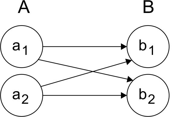
(a) $A\succeq_{1}B$

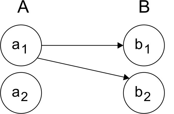
(b) $A\succeq_{2}B$

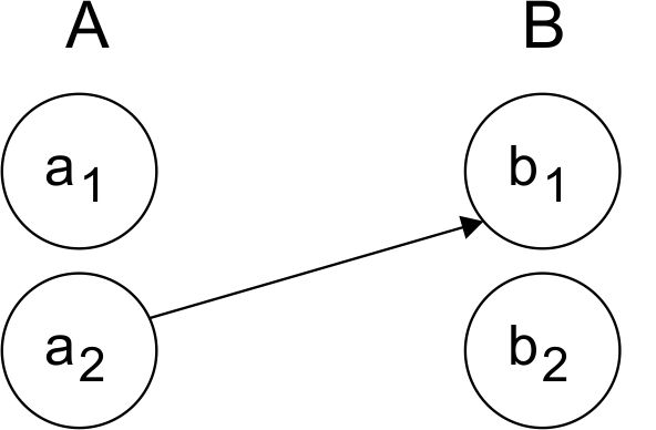
(c) $A\succeq_{4}B$

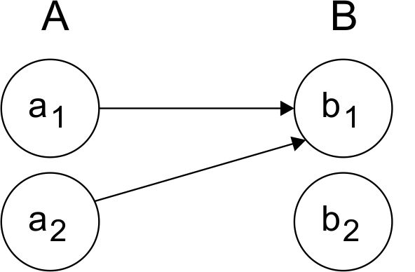
(d) $A\succeq_{5}B$

Figure 1. Examples of the extensions of $\succeq_{i}$. In this picture $a_{i}\rightarrow b_{j}$ means $a_{i}\succeq b_{j}$.

4.1. Univariate orders

Although stochastic dominance does not imply statistical preference in general, in the univariate case a number of sufficient conditions have been established for the implication, in terms of the copula that determines the joint distribution from the marginal ones. This is for instance the case when:

(SD-SP1):

$X$ and $Y$ are stochastically independent random variables, i.e., they are linked by the product copula (see [5, 7, 15]);

(SD-SP2):

$X$ and $Y$ are absolutely continuous random variables and they are coupled by an Archimedean copula (see [14]).

(SD-SP3):

$X,Y$ are either comonotonic or countercomonotonic, and they are both either simple or absolutely continuous.

In such cases, the implication transfers to the relations comparing sets of random variables, by means of the following lemma. Its proof is immediate and therefore omitted.

Lemma 3.

Let $\succeq$ be a preorder in a set $S$ and $A,B\subseteq S$. Let also $\sqsupseteq$ be a preorder that extends $\succeq$, i.e. $x\succeq y\Rightarrow x\sqsupseteq y\ \forall x,y\in S$. Then, $A\succeq_{i}B\Rightarrow A\sqsupseteq_{i}B$ for all $i=1,\ldots,6$.

Here $A$, $B$ are sets of random variables, denoted ${\mathcal{V}}_{\rm X}$, ${\mathcal{V}}_{\rm Y}$. The following special case of Lemma 3 is an instance.

Proposition 7.

Consider two sets of random variables ${\mathcal{V}}_{\rm X},{\mathcal{V}}_{\rm Y}$. Assume that any $X\in{\mathcal{V}}_{\rm X},Y\in{\mathcal{V}}_{\rm Y}$ satisfy one of the conditions (SD-SP1)$\div$(SD-SP3) above. Then, for all $i=1,\ldots,6$:

$${\mathcal{V}}_{\rm X}\succeq_{\rm SD_{i}}{\mathcal{V}}_{\rm Y}\Rightarrow{\mathcal{V}}_{\rm X}\succeq_{\rm SP_{i}}{\mathcal{V}}_{\rm Y}.$$

Proof.

As we have remarked, conditions (SD-SP1)$\div$(SD-SP3) above ensure that the statistical preference relation is an extension of stochastic dominance. The result follows from Lemma 3. ∎

4.2. Bivariate orders

Next we consider the following extension of stochastic dominance to the bivariate case:

Definition 12.

Let $X=(X_{1},X_{2})$ and $Y=(Y_{1},Y_{2})$ be two random vectors with respective bivariate distribution functions $F_{\rm X_{1},X_{2}}$ and $F_{\rm Y_{1},Y_{2}}$. We say that $(X_{1},X_{2})$ stochastically dominates $(Y_{1},Y_{2})$, and denote it $(X_{1},X_{2})\succeq_{\rm SD}(Y_{1},Y_{2})$, if $F_{\rm X_{1},X_{2}}(s,t)\leq F_{\rm Y_{1},Y_{2}}(s,t)$ for all $(s,t)\in\mathbb{R}^{2}$.

This definition establishes a way of comparing two bivariate vectors $X=(X_{1},X_{2})$, $Y=(Y_{1},Y_{2})$ in case their associated distribution functions are precisely known. However, it is not uncommon to have uncertain information about these distribution functions, that we can model by means of respective sets of distribution functions $\mathcal{F}_{\rm X},\mathcal{F}_{\rm Y}$. If we now take Definition 11 into account, we can propose a generalisation of Definition 12 to the imprecise case:

Definition 13.

Let $X=(X_{1},X_{2})$ and $Y=(Y_{1},Y_{2})$ be two random vectors with respective sets of bivariate distribution functions $\mathcal{F}_{\rm X},\mathcal{F}_{\rm Y}$. We say that $(X_{1},X_{2})$ i-stochastically dominates $(Y_{1},Y_{2})$, and denote it $(X_{1},X_{2})\succeq_{\rm SD_{i}}(Y_{1},Y_{2})$, if $\mathcal{F}_{\rm X}\leq_{\rm i}\mathcal{F}_{\rm Y}$.

Since by Remark 1 copulas can be interpreted as bivariate distribution functions, the extensions $\leq_{\rm i}$ are also applicable to them.

Note that the sets of distribution functions $\mathcal{F}_{\rm X},\mathcal{F}_{\rm Y}$ may be obtained by combining two respective marginal $p$-boxes by means of a set of copulas. In that case, we may study to which extent the relationships between the sets $\mathcal{F}_{\rm X},\mathcal{F}_{\rm Y}$ can be determined by means of the relationships between their marginal univariate $p$-boxes. In other words, if we have information stating that $X_{1}$ stochastically dominates $Y_{1}$ and $X_{2}$ stochastically dominates $Y_{2}$, we may wonder in which cases the pair $(X_{1},X_{2})$ $i$-stochastically dominates $(Y_{1},Y_{2})$. The following result gives an answer to this question:

Proposition 8.

Given two random vectors $X=(X_{1},X_{2})$, $Y=(Y_{1},Y_{2})$, let $(\underline{F}_{\rm X_{1}},\overline{F}_{\rm X_{1}}),(\underline{F}_{\rm X_{2}},\overline{F}_{\rm X_{2}}),(\underline{F}_{\rm Y_{1}},\overline{F}_{\rm Y_{1}})$, $(\underline{F}_{\rm Y_{2}},\overline{F}_{\rm Y_{2}})$ be the marginal $p$-boxes associated with $X_{1}$, $X_{2}$, $Y_{1}$, $Y_{2}$ respectively. Let $\mathcal{C}_{\rm X}$ and $\mathcal{C}_{\rm Y}$ be two sets of copulas. Define the following sets of bivariate distribution functions $\mathcal{F}_{\rm X},\mathcal{F}_{\rm Y}$:

$$\mathcal{F}_{\rm X} :=\{C(F_{\rm X_{1}},F_{\rm X_{2}}):C\in\mathcal{C}_{\rm X},F_{\rm X_{1}}\in(\underline{F}_{\rm X_{1}},\overline{F}_{\rm X_{1}}),F_{\rm X_{2}}\in(\underline{F}_{\rm X_{2}},\overline{F}_{\rm X_{2}})\},$$

$$\mathcal{F}_{\rm Y} :=\{C(F_{\rm Y_{1}},F_{\rm Y_{2}}):C\in\mathcal{C}_{\rm Y},F_{\rm Y_{1}}\in(\underline{F}_{\rm Y_{1}},\overline{F}_{\rm Y_{1}}),F_{\rm Y_{2}}\in(\underline{F}_{\rm Y_{2}},\overline{F}_{\rm Y_{2}})\}.$$

Consider $i\in\{1,\dots,6\}$ and assume that $(\underline{F}_{\rm X_{j}},\overline{F}_{\rm X_{j}})\leq_{\rm i}(\underline{F}_{\rm Y_{j}},\overline{F}_{\rm Y_{j}})$ for $j=1,2$. Then:

$$\mathcal{C}_{\rm X}\leq_{\rm i}\mathcal{C}_{\rm Y}\Rightarrow(X_{1},X_{2})\succeq_{\rm SD_{i}}(Y_{1},Y_{2}).$$

Proof.

• We know that:

  $$\begin{array}[]{l}\forall F_{\rm X_{j}}\in(\underline{F}_{\rm X_{j}},\overline{F}_{\rm X_{j}}),F_{\rm Y_{j}}\in(\underline{F}_{\rm Y_{j}},\overline{F}_{\rm Y_{j}}),F_{\rm X_{j}}\leq F_{\rm Y_{j}},(j=1,2);\\ \forall C_{\rm X}\in\mathcal{C}_{\rm X},C_{\rm Y}\in\mathcal{C}_{\rm Y},C_{\rm X}\leq C_{\rm Y},\\ \end{array}$$

  Consider $F_{\rm X}\in\mathcal{F}_{X}$ and $F_{\rm Y}\in\mathcal{F}_{Y}$. They can be expressed in the following way: $F_{\rm X}(x,y)=C_{\rm X}(F_{\rm X_{1}}(x),F_{\rm X_{2}}(y))$ and $F_{\rm Y}(x,y)=C_{\rm Y}(F_{\rm Y_{1}}(x),F_{\rm Y_{2}}(y))$, where $C_{\rm X}\leq C_{\rm Y}$. Then:

  $$\begin{array}[]{l c l}F_{\rm X}(x,y)&=&C_{\rm X}(F_{\rm X_{1}}(x),F_{\rm X_{2}}(y))\leq C_{\rm X}(F_{\rm Y_{1}}(x),F_{\rm Y_{2}}(y))\\ &\leq&C_{\rm Y}(F_{\rm Y_{1}}(x),F_{\rm Y_{2}}(y))=F_{\rm Y}(x,y),\end{array}$$

  where the inequalities hold because copulas are component-wise increasing.

• We know that:

  $$\begin{array}[]{l}\exists F_{\rm X_{j}}^{*}\in(\underline{F}_{\rm X_{j}},\overline{F}_{\rm X_{j}})\mbox{ s.t. }F_{\rm X_{j}}^{*}\leq F_{\rm Y_{j}}\quad\forall F_{\rm Y_{j}}\in(\underline{F}_{\rm Y_{j}},\overline{F}_{\rm Y_{j}}),(j=1,2).\\ \exists C_{\rm X}^{*}\in\mathcal{C}_{\rm X}\mbox{ s.t. }C_{\rm X}^{*}\leq C_{\rm Y}\quad\forall C_{\rm Y}\in\mathcal{C}_{\rm Y}.\end{array}$$

  Consider $F_{\rm X}(x,y):=C_{\rm X}^{*}(F_{\rm X_{1}}^{*}(x),F_{\rm X_{2}}^{*}(y))$, and let us see that $F_{\rm X}\leq F_{\rm Y}$ for any $F_{\rm Y}=C_{\rm Y}(F_{\rm Y_{1}},F_{\rm Y_{2}})$ in $\mathcal{F}_{Y}$:

  $$\begin{array}[]{lcl}F_{\rm X}(x,y)&=&C_{\rm X}^{*}(F_{\rm X_{1}}^{*}(x),F_{\rm X_{2}}^{*}(y))\leq C_{\rm X}^{*}(F_{\rm Y_{1}}(x),F_{\rm X_{2}}(y))\\ &\leq&C_{\rm Y}(F_{\rm Y_{1}}(x),F_{\rm X_{2}}(y))=F_{\rm Y}(x,y).\end{array}$$

• We know that:

  $$\begin{array}[]{l}\forall F_{\rm Y_{j}}\in(\underline{F}_{\rm Y_{j}},\overline{F}_{\rm Y_{j}}),\exists F^{*}_{\rm X_{j}}\in(\underline{F}_{\rm X_{j}},\overline{F}_{\rm X_{j}})\mbox{ s.t. }F^{*}_{\rm X_{j}}\leq F_{\rm Y_{j}},(j=1,2).\\ \forall C_{\rm Y}\in\mathcal{C}_{\rm Y}\ \exists C^{*}_{\rm X}\in\mathcal{C}_{\rm X}\mbox{ s.t. }C^{*}_{\rm X}\leq C_{\rm Y}.\end{array}$$

  Let $F_{\rm Y}\in\mathcal{F}_{Y}$. Then, there are $C_{\rm Y}\in\mathcal{C}_{Y},F_{\rm Y_{1}}\in(\underline{F}_{\rm Y_{1}},\overline{F}_{\rm Y_{1}})$ and $F_{\rm Y_{2}}\in(\underline{F}_{\rm Y_{2}},\overline{F}_{\rm Y_{2}})$ such that $F_{\rm Y}(x,y)=C_{\rm Y}(F_{\rm Y_{1}}(x),F_{\rm Y_{2}}(y))$. Let us check that there is $F_{\rm X}$ in $\mathcal{F}_{X}$ such that $F_{\rm X}\leq F_{\rm Y}$. Let $F_{\rm X}(x,y)=C^{*}_{\rm X}(F^{*}_{\rm X_{1}}(x),F^{*}_{\rm X_{2}}(y))$. Then:

  $$\begin{array}[]{lcl}F_{\rm X}(x,y)&=&C^{*}_{\rm X}(F^{*}_{\rm X_{1}}(x),F^{*}_{\rm X_{2}}(y))\leq C^{*}_{\rm X}(F_{\rm Y_{1}}(x),F_{\rm Y_{2}}(y))\\ &\leq&C_{\rm Y}(F_{\rm Y_{1}}(x),F_{\rm Y_{2}}(y))=F_{\rm Y}(x,y).\end{array}$$

• We know that:

  $$\begin{array}[]{l}\exists F_{\rm X_{j}}^{*}\in(\underline{F}_{\rm X_{j}},\overline{F}_{\rm X_{j}}),F_{\rm Y_{j}}^{*}\in(\underline{F}_{\rm Y_{j}},\overline{F}_{\rm Y_{j}})\mbox{ s.t. }F_{\rm X_{j}}^{*}\leq F_{\rm Y_{j}}^{*},(j=1,2).\\ \exists C_{\rm X}^{*}\in\mathcal{C}_{\rm X},C_{\rm Y}^{*}\in\mathcal{C}_{\rm Y}\mbox{ s.t. }C^{*}_{\rm X}\leq C^{*}_{\rm Y}.\end{array}$$

  Let us consider the distribution functions $F_{\rm X}(x,y)=C_{\rm X}^{*}(F_{\rm X_{1}}^{*}(x),F_{\rm X_{2}}^{*}(y))$ and $F_{\rm Y}(x,y)=C_{\rm Y}^{*}(F_{\rm Y_{1}}^{*}(x),F_{\rm Y_{2}}^{*}(y))$. It holds that $F_{\rm X}\leq F_{\rm Y}$:

  $$\begin{array}[]{lcl}F_{\rm X}(x,y)&=&C_{\rm X}^{*}(F_{\rm X_{1}}^{*}(x),F_{\rm X_{2}}^{*}(y))\leq C_{\rm X}^{*}(F_{\rm Y_{1}}^{*}(x),F_{\rm Y_{2}}^{*}(y))\\ &\leq&C_{\rm Y}^{*}(F_{\rm Y_{1}}^{*}(x),F_{\rm Y_{2}}^{*}(y))=F_{\rm Y}(x,y).\end{array}$$

• The proof of these two cases is analogous to that of $i=2$ and $i=3$, respectively. ∎

4.3. Natural extension and independent products

To conclude this section, we consider the particular cases discussed in Sections 3.2 and 3.3: those where the bivariate $p$-box is the natural extension or a factorising product.

By Proposition 5, the natural extension of two marginal $p$-boxes $(\underline{F}_{\rm X},\overline{F}_{\rm X})$ and $(\underline{F}_{\rm Y},\overline{F}_{\rm Y})$ is given by:

(17) $$\underline{F}(x,y)=C_{\rm L}(\underline{F}_{\rm X}(x),\underline{F}_{\rm Y}(y))\mbox{ and }\overline{F}(x,y)=C_{\rm M}(\overline{F}_{\rm X}(x),\overline{F}_{\rm Y}(y)).$$

This allows us to prove the following result:

Corollary 1.

Consider marginal $p$-boxes $(\underline{F}_{\rm X_{1}},\overline{F}_{\rm X_{1}}),(\underline{F}_{\rm X_{2}},\overline{F}_{\rm X_{2}}),(\underline{F}_{\rm Y_{1}},\overline{F}_{\rm Y_{1}})$ and $(\underline{F}_{\rm Y_{2}},\overline{F}_{\rm Y_{2}})$. Let $(\underline{F}_{\rm X},\overline{F}_{\rm X})$ (resp., $(\underline{F}_{\rm Y},\overline{F}_{\rm Y})$) be the natural extension of the $p$-boxes $(\underline{F}_{\rm X_{1}},\overline{F}_{\rm X_{1}}),(\underline{F}_{\rm X_{2}},\overline{F}_{\rm X_{2}})$ (resp., $(\underline{F}_{\rm Y_{1}},\overline{F}_{\rm Y_{1}}),(\underline{F}_{\rm Y_{2}},\overline{F}_{\rm Y_{2}})$) by means of Eq. (17). Then for $i=2,\dots,6$,

$$(\underline{F}_{\rm X_{j}},\overline{F}_{\rm X_{j}})\leq_{\rm i}(\underline{F}_{\rm Y_{j}},\overline{F}_{\rm Y_{j}}),j=1,2\Rightarrow(X_{1},X_{2})\succeq_{\rm SD_{i}}(Y_{1},Y_{2}).$$

Proof.

Take $\mathcal{C}_{\rm X}=\mathcal{C}_{\rm Y}=\{C_{\rm L},C_{\rm M}\}$ in Proposition 8. Since $C_{\rm L}\leq C_{\rm L}$, $C_{\rm M}\leq C_{\rm M}$ and $C_{\rm L}\leq C_{\rm M}$, we get $\mathcal{C}_{\rm X}\leq_{\rm i}\mathcal{C}_{\rm Y}$, $i=2,\ldots,6$. Then, Proposition 8 ensures $\{\underline{F}_{\rm X},\overline{F}_{\rm X}\}\leq_{\rm i}\{\underline{F}_{\rm Y},\overline{F}_{\rm Y}\}\ (i=2,\ldots,6)$. It is not difficult to check then that this implies also $(\underline{F}_{\rm X},\overline{F}_{\rm X})\leq_{\rm i}(\underline{F}_{\rm Y},\overline{F}_{\rm Y})\ (i=2,\ldots,6)$, because of the special form of $\mathcal{C}_{\rm X}$, $\mathcal{C}_{\rm Y}$. ∎

To see that the result does not hold for $\leq_{1}$, consider the following example:

Example 3.

For $j=1,2$, let $\underline{F}_{\rm X_{j}}=\overline{F}_{\rm X_{j}}=\underline{F}_{\rm Y_{j}}=\overline{F}_{\rm Y_{j}}$ be the distribution function associated with the uniform probability distribution on $[0,1]$, given by $F(x)=x$ for every $x\in[0,1]$. Then trivially

$$F=(\underline{F}_{\rm X_{j}},\overline{F}_{\rm X_{j}})\leq_{\rm 1}(\underline{F}_{\rm Y_{j}},\overline{F}_{\rm Y_{j}})=F\ \forall j=1,2.$$

However, $(\underline{F}_{\rm X},\overline{F}_{\rm X})\nleq_{\rm 1}(\underline{F}_{\rm Y},\overline{F}_{\rm Y})$, since $C_{\rm M}(F,F)\in(\underline{F}_{\rm X},\overline{F}_{\rm X}),C_{\rm L}(F,F)\in(\underline{F}_{\rm Y},\overline{F}_{\rm Y})$ and

$$C_{\rm M}(F,F)(0.5,0.5) =C_{\rm M}(F(0.5),F(0.5))=C_{\rm M}(0.5,0.5)=0.5>0$$

$$=C_{\rm L}(0.5,0.5)=C_{\rm L}(F(0.5),F(0.5))=C_{\rm L}(F,F)(0.5,0.5).\blacklozenge$$

On the other hand, Proposition 6 implies that, given two finite spaces $\mathcal{X},\mathcal{Y}$, any factorising coherent lower prevision $\underline{P}$ on $\mathcal{L}(\mathcal{X}\times\mathcal{Y})$ determines a bivariate $p$-box that is the product of its marginal $p$-boxes by means of the product copula. Taking this property into account, we can compare two factorising independent products in terms of the relationships between their marginals. From Proposition 8, we deduce the following:

Corollary 2.

Consider marginal $p$-boxes $(\underline{F}_{\rm X_{1}},\overline{F}_{\rm X_{1}}),(\underline{F}_{\rm Y_{1}},\overline{F}_{\rm Y_{1}})$, $(\underline{F}_{\rm X_{2}},\overline{F}_{\rm X_{2}})$ and $(\underline{F}_{\rm Y_{2}},\overline{F}_{\rm Y_{2}})$, and let us define the following sets of bivariate distribution functions $\mathcal{F}_{X},\mathcal{F}_{Y}$ by

$$\mathcal{F}_{X} :=\{F_{\rm X_{1}}\cdot F_{\rm X_{2}}:F_{\rm X_{1}}\in(\underline{F}_{\rm X_{1}},\overline{F}_{\rm X_{1}}),F_{\rm X_{2}}\in(\underline{F}_{\rm X_{2}},\overline{F}_{\rm X_{2}})\},$$

$$\mathcal{F}_{Y} :=\{F_{\rm Y_{1}}\cdot F_{\rm Y_{2}}:F_{\rm Y_{1}}\in(\underline{F}_{\rm Y_{1}},\overline{F}_{\rm Y_{1}}),F_{\rm Y_{2}}\in(\underline{F}_{\rm Y_{2}},\overline{F}_{\rm Y_{2}})\}.$$

Then, for $i=1,\dots,6$,

$$(\underline{F}_{\rm X_{j}},\overline{F}_{\rm X_{j}})\leq_{\rm i}(\underline{F}_{\rm Y_{j}},\overline{F}_{\rm Y_{j}}),j=1,2\Rightarrow(X_{1},X_{2})\succeq_{\rm SD_{i}}(Y_{1},Y_{2}).$$

Proof.

The result is the particular case of Proposition 8 where $\mathcal{C}_{X}=\mathcal{C}_{Y}=\{C_{\rm P}\}$. ∎

5. Conclusions and open problems

In this work we have studied the extension of Sklar’s theorem to an imprecise framework, where instead of random variables precisely described by their distribution functions, we have considered the case when they are imprecisely described by p-boxes. For this aim, we have introduced the notion of imprecise copula, and have proven that if we link two marginal p-boxes by means of a set of copulas we obtain a bivariate p-box whose associated lower probability is coherent. Unfortunately, the main implication of Sklar’s theorem does not hold in the imprecise framework: there exist coherent bivariate p-boxes that are not uniquely determined by their marginals.

We have investigated two particular cases: on the one hand, we considered the absence of information about the copula that links the marginals. In that case, we end up with the natural extension of the marginal p-boxes, that can be expressed in terms of the Łukasiewicz and the minimum copulas. On the other hand, we looked upon the case where the marginal distributions satisfy the condition of epistemic independence, and showed that the joint p-box can be obtained in most, but not all cases, by means of the product copula.

There are a few open problems that arise from our work in this paper: on the one hand, we should deepen the study of the properties of imprecise copulas from the point of view of aggregation operators. With respect to Sklar’s theorem, we intend to look for sufficient conditions for a bivariate p-box to be determined as an imprecise copula of its marginals. A third open problem would be the study in the imprecise case of the other extensions of stochastic dominance to the bivariate case, based on the comparisons of survival functions or expectations. Finally, it would be interesting to generalize our results to the $n$-variate case. An interesting work in this respect was carried out by Durante and Spizzichino in [9].

References

• [1] D. Álvarez. A Monte Carlo-based method for the estimation of lower and upper probabilities using infinite random sets of indexable type. Fuzzy Sets and Systems, 160:384–401, 2009.
• [2] I. Couso, S. Moral and P. Walley. A survey of concepts of independence for imprecise probabilities. Risk Decision and Policy, 5:165–181, 2000.
• [3] F. Cozman and C. de Campos. Kuznetsov independence for interval-valued expectations and sets of probability distributions: Properties and algorithms. International Journal of Approximate Reasoning, 55(2):666–682, 2014.
• [4] G. de Cooman, E. Miranda and M. Zaffalon. Independent natural extension. Artificial Intelligence, 175(12–13):1911–1950, 2011.
• [5] B. de Schuymer, H. de Meyer and B. de Baets. A fuzzy approach to stochastic dominance of random variables, pages 253–260. Lecture Notes in Artificial Intelligence 2715, 2003.
• [6] B. de Schuymer, H. de Meyer, B. de Baets and S. Jenei. On the cycle-transitivity of the dice model. Theory and Decision, 54:261–285, 2003.
• [7] B. de Schuymer, H. de Meyer and B. de Baets. Cycle-transitive comparison of independent random variables. Journal of Multivariate Analysis, 96:352–373, 2005.
• [8] D. Dubois, H. Fargier and P. Perny. Qualitative decision theory with preference relations and comparative uncertainty: An axiomatic approach. Artificial Intelligence, 148:219–260, 2003.
• [9] F. Durante and F. Spizzichino. Semi-copulas, capacities and families of level curves. Fuzzy Sets and Systems, 161(2):269–276, 2010.
• [10] S. Ferson, V. Kreinovich, L. Ginzburg, D. S. Myers and K. Sentz. Constructing probability boxes and Dempster-Shafer structures. Technical Report SAND2002–4015, Sandia National Laboratories, January 2003.
• [11] M. Fréchet. Généralisations du théorème des probabilités totales. Fundamenta Mathematicae, 25:379–387, 1935.
• [12] H. Levy. Stochastic dominance. Kluwer Academic Publishers, 1998.
• [13] E. Miranda and M. Zaffalon. Independent products on general spaces. 2014. Submitted for publication.
• [14] I. Montes, D. Martinetti, S. Díaz and S. Montes. Comparison of random variables coupled by archimedean copulas. In C. Borglet et al., editor, Combining Soth Computing and Statistical Methods in Data Analysis, volume 77 of Advances in Intelligent and Soft Computing, pages 467–474. Springer, 2010.
• [15] I. Montes, D. Martinetti, S. Díaz and S. Montes. Statistical preference as a tool in consensus processes. In E. Herrera et al., editor, Consensual processes, volume 267 of Studies in Fuzziness and Soft Computing, pages 65–92. Springer, 2011.
• [16] I. Montes, E. Miranda and S. Montes. Decision making with imprecise utilities and beliefs by means of statistical preference and stochastic dominance. European Journal of Operational Research, 234(1):209–220, 2014.
• [17] I. Montes, E. Miranda and S. Montes. Stochastic dominance with imprecise information. Computational Statistics and Data Analysis, 71(C):867–885, 2014.
• [18] A. Müller and D. Stoyan. Comparison Methods for Stochastic Models and Risks. Wiley, 2002.
• [19] R. Nelsen. An introduction to copulas. Springer, New York, 1999.
• [20] R. Nelsen, J. J. Quesada Molina, J. A. Rodríguez-Lallena and M. Úbeda Flores. Best-possible bounds on sets of bivariate distribution functions. Journal of Multivariate Analysis, 90:348–358, 2004.
• [21] R. Nelsen and M. Úbeda Flores. The lattice-theoretic structure of sets of bivariate copulas and quasi-copulas. C. R. Math. Acad. Sci. Paris, 341(9):583–586, 2005.
• [22] R. Pelessoni, P. Vicig, I. Montes and E. Miranda. Bivariate p-boxes. 2014. Submitted for publication.
• [23] M. Scarsini. Copulae of capacities on product spaces. In L. Rüschendorf, B. Schweizer, and M. D. Taylor, editors, Distributions with Fixed Marginals and Related Topics, volume 28 of IMS Lecture Notes- Monograph Series, pages 307–318. Institute of Mathematical Statistics, 1996.
• [24] B. Schmelzer. Joint distributions of random sets and their relation to copulas. In V.N. Huynh et al., editor, Modeling dependence in Econometrics, volume 251 of Advances in Intelligent Systems and Computing, pages 155–168. Springer, 2014.
• [25] M. Shaked and J. G. Shanthikumar. Stochastic Orders and their applications. Springer, 2006.
• [26] A. Sklar. Fonctions de répartition à n-dimensions et leurs marges. Publications de l’Institute de Statistique de l’Université de Paris, 8:229–231, 1959.
• [27] M. Troffaes and S. Destercke. Probability boxes on totally preordered spaces for multivariate modelling. International Journal of Approximate Reasoning, 52(6):767–791, 2011.
• [28] P. Walley. Statistical Reasoning with Imprecise Probabilities. Chapman and Hall, London, 1991.
• [29] R. Williamson. Probabilistic arithmetic. PhD thesis, University of Queensland, 1989.
• [30] R. R. Yager. Joint cumulative distribution functions for Dempster-Shafer belief structures using copulas. Fuzzy Optimization and Decision Making, 12:393–414, 2013.