Abstract: This paper presents an integral formulation for Helmholtz problems with mixed boundary conditions. Unlike most integral equation techniques for mixed boundary value problems, the proposed method uses a global boundary charge density. As a result, Calderón identities can be utilized to avoid the use of hypersingular integral operators. More importantly, the formulation avoids spurious resonances. Numerical results illustrate the performance of the proposed solution technique.

1. Introduction

This manuscript describes an integral equation technique for solving Helmholtz mixed boundary value problems for a scattering body $\Omega$ with boundary $\Gamma=\partial\Omega$. Specifically, we consider the following boundary value problem

(1) $$\left\{\begin{aligned} \Delta u+\omega^{2}u=&\ 0\qquad&&\mbox{ in }\Omega^{c},\\ u=&\ g\qquad&&\mbox{ on }\Gamma_{D},\\ \frac{\partial u}{\partial\nu}=&\ f\qquad&&\mbox{ on }\Gamma_{N},\\ \frac{\partial u}{\partial r}-i\omega u=&\ O\left(\frac{1}{r}\right)\qquad&&\mbox{ as }r\to\infty,\end{aligned}\right.$$

where $\Gamma_{D}$ denotes the portion of $\Gamma$ with Dirichlet boundary condition, $\Gamma_{N}$ denotes the portion of $\Gamma$ with Neumann boundary condition and $\Gamma=\Gamma_{D}\cup\Gamma_{N}$. The last equation in (1) is the outgoing Sommerfeld radiation condition which specifies a decay condition on the solution.

1.1. Prior work

Several integral equation based solution techniques have previously been used for solving mixed boundary value problems.

In [4, 12], Laplace mixed boundary value problems are considered. Both papers represent the solution as a linear combination of a double layer integral operator defined on $\Gamma_{D}$ with a single layer integral operator defined on $\Gamma_{N}$. The integral equation that results from enforcing boundary conditions involves evaluating a hypersingular integral operator which has a norm that can grow without bound even when considered on neighboring segments of $\Gamma$. By utilizing a near evaluation technique designed for the hypersingular operator and local compression, there does not appear to be a loss of accuracy associated with this solution technique.

The reformulation of Helmholtz boundary value problems as boundary integral equations needs to be done with some care to avoid introducing spurious resonances. A spurious resonance is a wavenumber $\omega$ for which a naïve integral equation formulation would result in a non-trivial null space even when the original boundary value problem is well-posed.

[10] considers (1) where $\Omega$ consists of a collection of scattering bodies and each body has a single type of boundary condition. To avoid spurious resonances, [10] uses a linear combination of combined field representations (one for $\Gamma_{D}$ and another for $\Gamma_{N}$). Roughly speaking, a block preconditioner involving two inverses is utilized to achieve a second kind integral equation for (1). Unfortunately, this technique does not extend directly to single body mixed boundary condition problems. [8] presents a similar approach for solving (1) on a single scattering body which utilizes a preconditioner that is equivalent to squaring the inverse of a first kind integral equation.

At this point, there does not appear to exist a uniquely solvable pure second kind integral equation for (1).

1.2. Outline

This paper presents an integral formulation for solving (1) which uses a single regularized combined field integral representation for the solution. Utilizing a Calderón identity leads to a simple block first kind integral equation system.

The manuscript begins by reviewing robust integral formulations for Dirichlet and Neumann boundary value problems in section 2. Then the proposed integral formulation is presented. Next, section 3 presents a technique for discretizing the resulting integral equation system. Finally, section 4 illustrates the performance of the proposed solution technique.

Remark 1.1.

While this paper focuses on Helmholtz problems with mixed Dirichlet and Neumann boundary data, the solution technique can easily be extended to case of additional Robin boundary conditions. Also, Laplace boundary value problems can be handled by setting $\omega=0$ and using the appropriate Green’s function.

2. Integral equation techniques

The reformulation of (1) as a block integral equation system involves the classical single, hypersingular and double layer kernels

(2) $$\begin{split}S_{\omega}f(x)&=\int_{\Gamma}G_{\omega}(x,y)f(y)ds(y),\\ T_{\omega}f(x)&=\eta_{x}\cdot\nabla_{x}\int_{\Gamma}\eta_{y}\cdot\nabla_{y}G_{\omega}(x,y)f(y)ds(y),\\ D_{\omega}f(x)&=\int_{\Gamma}\eta_{y}\cdot\nabla_{y}G_{\omega}(x,y)f(y)ds(y)\ \ \mbox{and}\\ D_{\omega}^{*}f(x)&=\int_{\Gamma}\eta_{x}\cdot\nabla_{x}G_{\omega}(x,y)f(y)ds(y)\end{split}$$

where $G_{\omega}(x,y)$ is the free space Green’s function

$$G_{\omega}(x,y)=\frac{\rm{i}}{4}H_{0}(\omega|x-y|)$$

of the two dimensional Helmholtz problem with wavenumber $\omega$ and $\eta_{p}$ denotes the outward facing normal vector at the point $p\in\Gamma$.

This section begins by presenting robust integral formulations for Dirichlet and Neumann boundary value problems. Then we propose a block integral equation system to solve (1).

2.1. The Dirichlet boundary value problem

Consider the Dirichlet boundary value problem

(3) $$\left\{\begin{aligned} \Delta u+\omega^{2}u=&\ 0\qquad&&\mbox{ in }\Omega^{c},\\ u=&\ g\qquad&&\mbox{ on }\Gamma,\\ \frac{\partial u}{\partial r}-i\omega u=&\ O\left(\frac{1}{r}\right)\qquad&&\mbox{ as }r\to\infty,\end{aligned}\right.$$

where $\omega$ denotes the constant wavenumber.

The solution can be represented as a combined field

(4) $$u(x)=D_{\omega}\sigma(x)-i|\omega|S_{\omega}\sigma(x),$$

where $\sigma(x)$ is an unknown boundary charge density.

It is well-known [11, 2] that a uniquely solvable boundary integral equation

(5) $$\frac{1}{2}\sigma(x)+D_{\omega}\sigma(x)-i|\omega|S_{\omega}\sigma(x)=g(x)$$

for $\sigma(x)$ results from enforcing the boundary condition. The integral equation (5) is second kind on smooth $\Gamma$ and is sometimes referred to as the Combined Field Integral Equation.

2.2. The Neumann boundary value problem

Consider the Neumann boundary value problem

(6) $$\left\{\begin{aligned} \Delta u+\omega^{2}u=&\ 0\qquad&&\mbox{ in }\Omega^{c},\\ \frac{\partial u}{\partial\nu}=&\ f\qquad&&\mbox{ on }\Gamma,\\ \frac{\partial u}{\partial r}-i\omega u=&\ O\left(\frac{1}{r}\right)\qquad&&\mbox{ as }r\to\infty,\end{aligned}\right.$$

where $\omega$ denotes the constant wavenumber, and $\nu$ denotes the outward facing normal vector for $x\in\Gamma$.

Using the combined field representation (4) for the solution of (6) results in the integral equation

(7) $$-i|\omega|\left(-\frac{1}{2}\sigma(x)+D^{*}_{\omega}\sigma(x)\right)+T_{\omega}\sigma(x)=f(x)$$

which is not a second kind integral equation for smooth $\Gamma$ since the hypersingular integral operator $T_{\omega}$ is not compact. The $T_{\omega}$ operator is troublesome for two reasons. First, $T_{\omega}$ is an unbounded operator from $L^{2}(\Gamma)$ to $L^{2}(\Gamma)$. As a direct consequence, the linear system resulting from discretization of the integral equation (7) is ill-conditioned. Second, standard singular quadrature such as [9] are not sufficient to discretize the operator. While it is possible to overcome both these difficulties by developing analytical and quadrature techniques which view $T_{\omega}$ as an operator between two Sobolev spaces, there are highly accessible alternatives.

The most common approach to avoid these problems is to utilized a so-called regularized combined field representation

(8) $$u(x)=D_{\omega}S_{\omega}\sigma(x)-i|\omega|S_{\omega}\sigma(x)$$

where $\sigma(x)$ still represents an unknown boundary charge distribution. Enforcing the Neumann boundary condition results in a regularized boundary integral equation

(9) $$-i|\omega|\left(-\frac{1}{2}\sigma(x)+D^{*}_{\omega}\sigma(x)\right)+T_{\omega}S_{\omega}\sigma(x)=f(x).$$

This integral equation is called regularized because upon utilizing Calderón identities [11] we can rewrite (9) as

(10) $$\left(\frac{1}{4}+i|\omega|\frac{1}{2}\right)\sigma(x)-i|\omega|D^{*}_{\omega}\sigma(x)+(D^{*}_{\omega})^{2}\sigma(x)=f(x).$$

which does not involve hypersingular integral operators.

On smooth geometries, equation (10) is a second kind integral equation.

2.3. The mixed boundary value problem

For the mixed boundary value problem (1), we choose to use the regularized combined field representation (8) for the solution. With this choice, we are able to utilize to two very appealing properties: (i) it avoids spurious resonances and (ii) special quadrature for hypersingular integral operators is not needed. The compromise is that the resulting integral equation has a first kind block.

From section 2.2, we know the block row integral equation for $x\in\Gamma_{N}$ is given by equation (9).

Applying (8) to $\Gamma_{D}$ results in a first kind integral equation given by

(11) $$\frac{1}{2}S_{\omega}\sigma(x)+D_{\omega}S_{\omega}\sigma(x)-i|\omega|S_{\omega}\sigma(x)=f(x).$$

Rewriting the integral equation in block form, we get

(12) $$\left[\begin{array}[]{cc}S^{D}_{\omega}+(D_{\omega}S_{\omega})^{D}-i|\omega|S_{\omega}^{D}\\ (\frac{1}{4}+i|\omega|\frac{1}{2})I^{N}-i|\omega|D^{*,N}_{\omega}+(D^{*}_{\omega})^{2,N}\end{array}\right]\sigma=\left[\begin{array}[]{cc}g\\ f\end{array}\right]$$

where

$$S_{\omega}^{D}\sigma(x)=\int_{\Gamma}G_{\omega}(x,y)\sigma(y)ds(y)\ {\rm for}\ x\in\Gamma_{D},$$

$$D^{*,N}_{\omega}\sigma(x)=\int_{\Gamma}G_{\omega}(x,y)\sigma(y)ds(y)\ {\rm for}\ x\in\Gamma_{N},$$

$$(D_{\omega}S_{\omega})^{D}\sigma(x)=\int_{\Gamma}\eta_{y}\cdot\nabla_{y}G_{\omega}(x,y)\left(\int_{\Gamma}G_{\omega}(y,w)\sigma(w)ds(w)\right)ds(y)\ x\in\Gamma_{D}$$

etc.

Let $\bm{\mathsf{A}}\bm{\mathsf{\sigma}}=\bm{\mathsf{b}}$ denote the condensed form of (12).

3. Discretization

Some care needs to be taken when discretizing the block integral equation (12) since the boundary charge distribution $\sigma$ is likely to not be smooth at the Dirichlet-Neumann junctions. Figure 1 illustrates the behavior of the boundary charge distribution $\sigma$ when $\omega=1$ and half a smooth star geometry (see Figure 3(a)) has zero Neumann boundary condition while the remainder has a Dirichlet boundary condition generated by a solution a free space Helmholtz problem. We follow the approach of [1, 6, 7, 5, 3] which describe techniques for dealing with the singularities that occur when solving scattering problems on Lipschitz geometries. Thus a standard panel based quadrature rule is used for the Nyström discretization of (12). Near the Dirichlet-Neumann junctions the mesh is refined until the contribution from the panels closest to the junctions is small.

Figure 1. Illustration of $|\sigma|$ on $\Gamma_{D}$ (solid line) and $\Gamma_{N}$ (dashed line) vs the distance $r$ from the Dirichlet-Neumann Junction on the left-hand side (a) and right-hand side (b) of the star geometry (see Figure 3)(a) when $\omega=1$ and the solution is unknown (see section 4.1 for problem specifications). Four levels of dyadic refinement are utilized making the closest points to the junctions $r=10^{-8}$ away.

For simplicity of presentation, consider a geometry where $\Gamma_{D}$ is comprised solely of one section of $\Gamma$ and (by default) $\Gamma_{N}$ is also one portion of $\Gamma$ as in Figure 3. First the geometry is partitioned into the six pieces such that $\Gamma_{1}\cup\Gamma_{2}\cup\Gamma_{3}=\Gamma_{D}$ and $\Gamma_{4}\cup\Gamma_{5}\cup\Gamma_{6}=\Gamma_{N}$. $\Gamma_{2}$ and $\Gamma_{5}$ are the parts of $\Gamma$ not directly touching the boundary condition junctions, while the pairs $\{\Gamma_{1},\Gamma_{6}\}$ and $\{\Gamma_{3},\Gamma_{4}\}$ join at boundary condition junctions. Hence $\Gamma_{s}=\Gamma_{2}\cup\Gamma_{5}$ is the portion of $\Gamma$ where the solution $\sigma$ is smooth and $\Gamma_{r}=\Gamma_{1}\cup\Gamma_{3}\cup\Gamma_{4}\cup\Gamma_{6}$ is the portion of $\Gamma$ where local refinement is likely needed. Figure 2(a) illustrates the partitioning of $\Gamma$ for the smooth star geometry where the upper half of $\Gamma$ has Neumann boundary conditions while the lower half of $\Gamma$ has Dirichlet boundary conditions. Since $\sigma$ is smooth on $\Gamma_{s}$, this region can be discretized coarsely. For the portions of the boundary near the boundary condition junctions $\Gamma_{r}$, the panels nearest to the junctions are recursively cut in half until the contribution from the panel nearest the junction is so small that it can be ignored. For many problems on smooth geometries, it is sufficient to stop $10^{-8}$ away from the junction point to obtain eight digits of accuracy. Referencing the third column of table 1, we note that using four levels of refinement corresponding to being approximately $10^{-8}$ away from the junctions does result in eight digits of accuracy.

Figure 2(b) illustrates the discretization with three levels of refinement into the junctions. Figure 2(c) is a zoomed in view of the left-hand side of the same figure. Note that this refinement procedure introduces a superfluous amount of points near the junctions. The extra points can be eliminated via compression techniques presented in [1, 6, 7, 5, 3]. Since the focus of this paper is on the performance of the integral formulation, no compression techniques are utilized in the numerical experiments in section 4.

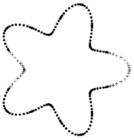
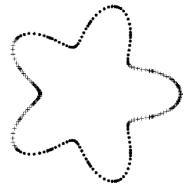
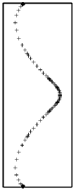
(a)		(b)		(c)

Figure 2. Illustration of the discretization for a smooth star geometry with $\Gamma_{N}$ corresponding to the upper half of $\Gamma$ and $\Gamma_{D}$ corresponding to the lower half of $\Gamma$ where $\bullet$ are nodes in $\Gamma_{s}$ and $+$ are nodes in $\Gamma_{r}$. (a) A 10 point composite Gaussian grid with no refinement. (b) The three level locally refined grid. (c) A closer view of the locally refined grid.

4. Numerical examples

This section reports on the performance of the purposed solution technique for solving boundary value problems with mixed boundary data. Section 4.1 considers the Helmholtz problem with mixed boundary conditions for three geometries, a smooth star, a pacman and a tear geometry. These geometries represent the three most common boundary phenomena: smooth boundary, a re-entrant corner, and a corner with the possibility of confined oscillations. Performance of the solution technique for the boundary conditions corresponding to a smooth known solution and an unknown solution are presented. Section 4.2 considers a Laplace problem with mixed boundary conditions on a smooth geometry. A comparison of the performance of the proposed method versus the integral formulation proposed in [4] is reported.

All integral equations are discretized using a Nyström technique based on a 16-point composite Gaussian quadrature [9]. Panels are placed on the geometries via the method described in section 3. The number of discretization points is $N=16(N_{\rm pan}+4(2^{l}))$ where $N_{\rm pan}$ is the number of panels on $\Gamma_{s}$ and $2^{l}$ is the number of refinement panels utilized.

The experiments were run on a Lenovo laptop computer with 16GB of RAM and a 2.4GHz Intel i7-4700M procesor in Matlab.

4.1. Helmholtz problems

This section considers the mixed boundary value problem (1) with three different wave numbers ($\omega=1$, $10$, and $100$) on three geometries:

• Illustrated in see Figure 3 (a), the smooth star geometry is given by the parameterization $\left(x(t),y(t)\right)=\left(1+0.3\cos(5t))\cos(t),\sin(t)(1+0.3\cos(5*t)\right)$ where $-\pi<t<\pi$.

• Illustrated in see Figure 3 (b), the tear geometry is given by the parameterization $\left(x(t),y(t)\right)=\left(2{\rm sign}(t)\sin(t),-\tan(\pi/4)\sin(2t)\right)$ where $-\pi<t<\pi$.

• Illustrated in see Figure 3 (c), the pacman geometry is given by the parameterization $\left(x(t),y(t)\right)=\left({\rm sign}(t)\sin(1.5t),\tan(3\pi/2)\sin(t)\right)$ where $-\pi<t<\pi$.

The Dirichlet-Neumann junctions occur at $t=0$ and $t=-\pi$ in parameter space so that half the boundary has Dirichlet boundary conditions while the other half has Neumann boundary conditions. For each wavenumber/geometry combination, two types of boundary data are considered:

• Both the Dirichlet and Neumann boundary are generated by a known solution to the Helmholtz problem corresponding to a collection of ten point charges inside of the geometry.

• The Dirichlet boundary data is generated by the same ten point charges but the Neumann data is set to zero. Hence, the solution is not known a priori.

For each wavenumber/geometry combination, tables 1-3 report

• The number of levels of refinement into the Dirichlet-Neumann junctions.

• The total number of discretization points.

• The relative error $E_{\rm rel}=\frac{\|u_{l}-u_{\rm ex}\|}{\|u_{\rm ex}\|}$ for the known solution problem where $u_{l}$ is the approximate solution, with $l$ levels of refinement, at twenty locations outside the geometry and $u_{\rm ex}$ is the exact solution at the twenty locations outside the geometry generated by the ten interior point charges.

• The relative convergence error $E_{\rm conv}=\frac{\|u_{l}-u_{l-1}\|}{\|u_{l}\|}$ where $u_{l}$ is the approximate solution, with $l$ levels of refinement, at twenty locations outside the geometry.

• The condition number $\kappa(\bm{\mathsf{A}})$ of linear system resulting from the discretization of (12).

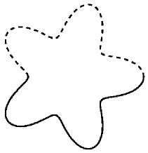
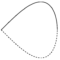
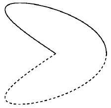
(a)	(b)	(c)

Figure 3. The contours $\Gamma$ used in the numerical experiments in Section 4. (a) Smooth star. (b) Tear. (c) Pacman. The portion of the boundary with the dashed line has Neumann boundary conditions while the portion of the boundary with solid line has Dirichlet boundary conditions.

	$\omega=1$				$\omega=10$
$l$	$N$	$E_{\rm rel}$	$E_{\rm conv}$	$\kappa(\bm{\mathsf{A}})$	N	$E_{\rm rel}$	$E_{\rm conv}$	$\kappa(\bm{\mathsf{A}})$
0	416	7.05e-10	1.00e-04	3.06e03	576	3.91e-10	1.21e-04	4.35e03
1	480	7.05e-10	7.55e-05	8.35e03	640	3.91e-10	9.04e-04	1.13e04
2	608	7.05e-10	2.36e-05	4.30e04	768	3.91e-10	2.82e-05	5.18e04
3	864	7.05e-10	1.57e-06	7.05e05	1024	3.91e-10	1.88e-06	8.38e05
4	1376	7.05e-10	6.13e-09	1.80e08	1536	3.91e-10	7.36e-09	2.14e08
5	2400	7.05e-10	-	1.18e13	2560	3.91e-10	-	1.40e13

	$\omega=100$
$l$	$N$	$E_{\rm rel}$	$E_{\rm conv}$	$\kappa(\bm{\mathsf{A}})$
0	2656	3.93e-10	9.68e-05	4.95e04
1	2720	3.93e-10	7.25e-05	1.01e05
2	2848	3.93e-10	2.27e-05	4.06e05
3	3104	3.93e-10	1.51e-06	6.49e06
4	3616	3.93e-10	5.91e-09	1.66e09
5	4640	3.93e-10	-	1.08e14

Table 1. The number of the levels of refinement $l$ into Dirichlet-Neumann junctions, the number of discretization points $N$, the relative error $E_{\rm rel}$ for the boundary value problem with known solution, the relative convergence error $E_{\rm conv}$ for the boundary value problem with unknown solution and the condition number $\kappa(\bm{\mathsf{A}})$ of the linear system resulting from the discretization of the integral equation (12) on the smooth star geometry for three wave numbers $\omega=1,10,$ and $100$.

	$\omega=1$				$\omega=10$
$l$	$N$	$E_{\rm rel}$	$E_{\rm conv}$	$\kappa(\bm{\mathsf{A}})$	N	$E_{\rm rel}$	$E_{\rm conv}$	$\kappa(\bm{\mathsf{A}})$
1	320	4.48e-06	2.93e-04	3.17e03	320	1.89e-07	1.59e-03	2.19e03
2	448	1.89e-06	1.79e-04	1.26e04	488	4.37e-08	8.82e-04	8.70e03
3	704	8.73e-08	3.91e-05	2.01e05	704	2.58e-09	1.62e-04	1.39e05
4	1216	5.22e-10	1.34e-06	5.14e07	1216	1.19e-11	4.52e-06	3.56e07
5	2240	4.13e-11	3.04e-08	3.37e12	2240	7.37e-12	7.027e-08	2.34e12

	$\omega=100$
$l$	$N$	$E_{\rm rel}$	$E_{\rm conv}$	$\kappa(\bm{\mathsf{A}})$
1	2080	1.43e-09	1.11e-03	3.35e04
2	2208	8.26e-10	6.21e-04	1.34e05
3	2464	7.67e-10	1.13e-04	2.15e06
4	2976	7.67e-10	2.89e-06	5.49e08
5	4000	7.67e-10	2.74e-07	3.55e13

Table 2. The number of the levels of refinement $l$ into Dirichlet-Neumann junctions, the number of discretization points $N$, the relative error $E_{\rm rel}$ for the boundary value problem with known solution, the relative convergence error $E_{\rm conv}$ for the boundary value problem with unknown solution and the condition number $\kappa(\bm{\mathsf{A}})$ of the linear system resulting from the discretization of the integral equation (12) on the tear geometry for three wave numbers $\omega=1,10,$ and $100$.

	$\omega=1$				$\omega=10$
$l$	$N$	$E_{\rm rel}$	$E_{\rm conv}$	$\kappa(\bm{\mathsf{A}})$	N	$E_{\rm rel}$	$E_{\rm conv}$	$\kappa(\bm{\mathsf{A}})$
1	384	2.23e-04	2.93e-04	4.93e03	384	4.59e-04	3.61e-04	4.13e03
2	512	9.65e-05	1.79e-04	2.02e04	512	1.95e-04	1.79e-04	1.69e04
3	768	1.74e-05	3.91e-05	3.23e05	768	3.55e-05	3.42e-05	2.71e05
4	1280	5.82e-07	1.34e-06	8.28e07	1280	1.17e-06	1.14e-06	6.94e07
5	2304	1.39e-08	3.04e-08	5.43e12	2304	1.34e-09	1.11e-07	4.56e12

	$\omega=100$
$l$	$N$	$E_{\rm rel}$	$E_{\rm conv}$	$\kappa(\bm{\mathsf{A}})$
1	2080	5.71e-06	8.59e-05	5.91e04
2	2208	2.40e-06	2.67e-05	2.36e05
3	2464	4.38e-07	1.79e-06	3.79e06
4	2976	1.62e-08	1.89e-08	9.69e08
5	4000	7.06e-09	1.96e-08	6.26e13

Table 3. The number of the levels of refinement $l$ into Dirichlet-Neumann junctions, the number of discretization points $N$, the relative error $E_{\rm rel}$ for the boundary value problem with known solution, the relative convergence error $E_{\rm conv}$ for the boundary value problem with unknown solution and the condition number $\kappa(\bm{\mathsf{A}})$ of the linear system resulting from the discretization of the integral equation (12) on the pacman geometry for three wave numbers $\omega=1,10,$ and $100$.

For the smooth star geometry (table 1), the proposed method is able to capture the smooth known solution without refinement independent of wavenumber. The tear and pacman geometries have corners that require refinement into the corners in order to capture the known solution since the boundary charge distribution $\sigma$ is not smooth in the corner. Since $\sigma$ is smooth at the Dirichlet-Neumann junction away from the corner, the same performance would be observed if the refinement was only in the corner.

For the unknown solution experiments, the boundary charge distribution is not smooth for any of the geometries. Thus refinement into the Dirichlet-Neumann junctions is required to get high accuracy for all the experiments. The performance of the proposed method is similar to its performance on the experiments with known solution on a geometry with a corner.

The condition number of the linear system grows with the increased refinement into the Dirichlet-Neumann junctions. This behavior is expected given the first kind nature of the integral equation.

4.2. Laplace boundary value problem

This section reports on the performance of the proposed method and the integral formulation proposed in [4] for Laplace problems on the smooth star geometry with boundary data as specified by the known solution and unknown solution problems in the previous section. It should be noted that [4] uses a special quadrature to handle the hypersingular integral operator. The results reported in this section use the same Nyström discretization with 16-point composite Gaussian quadrature [9] for both integral equations. The results using the integral formulation from [4] have an $H$ superscript.

As with the Helmholtz boundary value problem, the proposed method does not require refinement when the boundary charge distribution is smooth. When the boundary charge distribution is not smooth, refinement allows for technique to capture the solution to high accuracy. This is contrast to the integral formulation from [4] which requires refinement to achieve high accuracy independent on whether or not the solution is smooth. Note that while the integral formulation from [4] is block second kind, since the hypersingular term has not been dealt with specially, the condition number for the discretized linear system is nearly squared that of the first kind system.

l	N	$E_{\rm rel}$	$\kappa(\bm{\mathsf{A}})$	$E^{H}_{\rm rel}$	$\kappa(\bm{\mathsf{A}}^{H})$	$E_{\rm conv}$	$E^{H}_{\rm conv}$
0	352	3.33e-10	9.21e02	8.07e-05	6.78e04	1.49e-06	4.18e-03
1	416	3.33e-10	2.81e03	4.04e-05	2.71e05	1.12e-06	1.62e-04
2	544	3.33e-10	1.28e04	1.01e-05	4.33e06	3.49e-07	5.07e-05
3	800	3.33e-10	2.12e05	6.31e-07	1.11e09	2.32e-08	3.37e-06
4	1312	3.33e-10	5.44e07	2.45e-09	7.27e13	1.16e-11	1.33e-08
5	2336	3.33e-10	3.57e12	1.69e-11	3.12e23	-	-

Table 4. The number of the levels of refinement $l$ into Dirichlet-Neumann junctions, the number of discretization points $N$, the relative error $E_{\rm rel}$ for the Laplace boundary value problem with known solution, the relative convergence error $E_{\rm conv}$ for the Laplace boundary value problem with unknown solution and the condition number $\kappa(\bm{\mathsf{A}})$ of the linear system resulting from the discretization of the integral equation (12) on the star geometry. The values with the superscript $H$ correspond to the results from using the integral formulation from [4].

5. Concluding remarks

This paper presented a robust integral equation formulation for solving mixed boundary value problems of the form of (1). The formulation is a direct extension of the integral equation techniques for single boundary condition scattering problems. Numerical results show that high accuracy can be obtained by utilizing local refinement near boundary condition junctions even if the junction is at a corner.

If one does not have access to discretization techniques for hypersingular kernels, the proposed solution technique is a high accuracy option for Laplace problems with mixed boundary value problems.

References

- [1] J. Bremer. A fast direct solver for the integral equations of scattering theory on planar curves with corners. J. Comput. Phys., 231:1879–1899, 2012.
- [2] D. Colton and R. Kress. Inverse Acoustic and Electromagnetic Scattering Theory. Springer-Verlag, New York, 2nd edition, 1998.
- [3] A. Gillman, S. Hao, and P. Martinsson. A simplified technique for the efficient and high-order accurate discretization of boundary integral equations in 2d on domains with corners. J. Comput. Phys., 256:214–219, 2014.
- [4] J. Helsing. Integral equation methods for elliptic problems with boundary conditions of mixed type. J. Comput. Phys., 228:8892–8907, 2009.
- [5] J. Helsing. The effective conductivity of arrays of squares: large random unit cells and extreme contrast ratios. J. Comput. Phys., 230(20):7533–7547, 2011.
- [6] J. Helsing. A fast and stable solver for singular integral equations on piecewise smooth curves. SIAM J. Sci. Comput., 33(1):153–174, 2011.
- [7] J. Helsing and R. Ojala. Corner singularities for elliptic problems: Integral equations, graded meshes, quadrature, and compressed inverse preconditioning. J. Comput. Phys., 227(20):8820 – 8840, 2008.
- [8] A. Kleefeld. The exterior problem for the helmholtz equation with mixed boundary conditions in three dimensions. Int. J. Comput. Math, 00:1–20, 2011.
- [9] P. Kolm and V. Rokhlin. Numerical quadratures for singular and hypersingular integrals. Comput. Math. Appl., 41:327–352, 2001.
- [10] R. Kress and G. Roach. On mixed boundary value problems for the helmholtz equation. P. Roy. Soc. Edinb. A, 77:65–77, 1977.
- [11] J.-C. Nédélec. Acoustic and Electromagnetic Equations: Integral Representations for Harmonic Functions. Springer, New York, 2012.
- [12] R. Ojala. A robust and accurate solver of laplace’s equation with general boundary conditions on general domains in the plane. J. Comput. Math., 30:433 – 448, 2012.