Photo-ionization of planetary winds: case study HD 209458b

Abstract

Close-in hot Jupiters are exposed to a tremendous photon flux that ionizes the neutral escaping material from the planet leaving an observable imprint that makes them an interesting laboratory for testing theoretical models. In this work we present 3D hydrodynamic simulations with radiation transfer calculations of a close-in exoplanet in a blow-off state. We calculate the Ly-$\alpha$ absorption and compare it with observations of HD 209458b and previous simplified model results. Our results show that the hydrodynamic interaction together with a proper calculation of the photoionization proccess are able to reproduce the main features of the observed Ly-$\alpha$ absorption, in particular at the blue-shifted wings of the line. We found that the ionizing stellar flux produce an almost linear effect on the amount of absorption in the wake. Varying the planetary mass loss rate and the radiation flux, we were able to reproduce the $10\%$ absorption observed at $-100\leavevmode\nobreak\ \mathrm{km\leavevmode\nobreak\ s^{-1}}$.

1 Introduction

The discovery of the first hot Jupiter transiting its host star HD 209458 took place more than a decade ago (see Charbonneau et al., 2000; Henry et al., 2000). The analysis of data samples of the extra-solar planet transit HD 209458b obtained with the Space Telescope Imaging Spectrograph on board of the Hubble Space Telescope made by Vidal-Madjar et al. (2003) revealed the existence of an extended upper atmosphere, and opened a discussion on whether the atmosphere is being lost (see Ben-Jaffel, 2007, 2008). Vidal-Madjar et al. (2008) revisited the observations and the theoretical- works based on the picture of an escaping atmosphere (e.g. Lammer et al., 2003; Lecavelier des Etangs et al., 2004; Yelle, 2004, 2006; Baraffe et al., 2005; Tian et al., 2005; Schneiter et al., 2007; García Muñoz, 2007) and confirmed it. Since then numerous theoretical works have been carried out shifting the discussion to the escaping mechanism, putting the focus on trying to explain the absorption produced at high velocities (see Holmström et al., 2008; Ekenbäck et al., 2010; Tremblin & Chiang, 2013; Villarreal D’Angelo et al., 2014; Bourrier & Lecavelier des Etangs, 2013). Vidal-Madjar et al. (2008) evaluated the absorption seen during transit within the ‘blue’ and the ‘red’ sides (of the wavelength domain defined in Ben-Jaffel, 2007) finding a $9.8\pm 1.8\%$ and $5.2\pm 1.0\%$ absorption, respectively.

Vidal-Madjar et al. (2003) first interpreted the absorption as hydrogen atoms in the exosphere undergoing hydrodynamic escape, accelerated by the stellar radiation pressure. Later, Schneiter et al. (2007) developed a 3D hydrodynamic model of the interaction between the stellar wind and the gas escaping from the planet (HD 209458b). By comparing the calculated Ly-$\alpha$ absorption with the observations they were able to estimate an upper limit for the planetary mass loss rate ($\dot{M}_{\mathrm{p}}$). In Villarreal D’Angelo et al. (2014) the stellar wind conditions were improved by comprehensively studying the stellar wind parameters. This was done by using a polytropic model to estimate the initial conditions for the stellar wind at the radial distance (from the centre of the star) at which it was imposed. Several stellar wind velocities where tested together with the coupled stellar wind temperature ($T_{*}$), finding a suitable range for $\dot{M}_{\mathrm{p}}$ ($[3$–$5]\times 10^{10}$ g s^-1). Schneiter et al. (2007) and Villarreal D’Angelo et al. (2014), distinguished the planetary wind from the stellar wind with the aid of a passive scalar, and calculated the Ly-$\alpha$ absorption assuming that all neutral material with temperatures above $10^{5}\leavevmode\nobreak\$K was ionized. These works were able to reproduce the velocity range of neutral planetary atoms responsible for the observed absorption in the Ly-$\alpha$ line.

The work done in Holmström et al. (2008) and its follow up Ekenbäck et al. (2010) reproduce the absorption observed at Doppler shift $-100\leavevmode\nobreak\$km s^-1. They simulated the production of energetic neutral hydrogen (ENAs) through charge exchange between stellar wind protons and exospheric hydrogen, assuming stellar wind conditions similar to those at an equivalent distance in our Sun. Tremblin & Chiang (2013) further explored the charge-exchange scenario by means of a 2D hydrodynamic model, making emphasis on the mixing layer between both winds.

Bourrier & Lecavelier des Etangs (2013) presented a 3D Monte-Carlo numerical particle model developed to simu-late the escaping gas of an exoplanet. In their model the focus was set on the radiation pressure, taking into account the ionization, the self-shielding, and the stellar wind interaction. The charge-exchange process was included as an impulse given by the incoming stellar wind proton, aiming, this way, to explain the blue-shifted absorption.

Even though most of these models employ different acceleration mechanism for the neutral particles, they all have been capable of reproducing the global structure of the upper atmosphere of exoplanets undergoing mass loss due to Roche lobe overflow, predicting planetary mass loss rates in the range $10^{9}$–$10^{11}$ g s^-1, leaving the question of which particle acceleration mechanism is responsible for the absorption at high Doppler shift, still open.

Recent progress has been made to model the planetary mass loss rate including the effect of magnetic fields in both the star and the planet. It has been shown for instance that space weather events (such as CME) or the parameters of the planetary system itself, can have an influence on the mass loss from the planet (see for example Cohen et al., 2011a, b; Owen & Adams, 2014; Trammell et al., 2014; Adams, 2011; Matsakos et al., 2015). Owen & Adams (2014) find, through a number of numerical simulations that include the stellar UV flux, that the presence of magnetic fields, can reduce the amount of planetary mass loss rate by aproximately an order of magnitude if the planet can sustain moderate magnetic fields values ($B_{p}>1\leavevmode\nobreak\ G$). Finally, as mentioned in Cohen et al. (2011a, b) and in Owen & Adams (2014), the interaction of the planetary magnetosphere with the magnetized stellar wind is expected to be highly dynamic and change with time according to the parameters of the planetary system.

Here we present a 3D numerical model of the hydrodynamic interaction between the winds that includes in a self-consistent manner the calculation of the photo-ionization, and we focus in the effects of varying the ionizing flux, the stellar wind parameters and the mass loss rate of the planet. Similar simulations have recently been presented by Tripathi et al. (2015), where the evaporation of the exoplanet atmosphere is modeled with radiation hydrodynamics. In such work, an asymmetric planetary wind is produced by a plane parallel radiative field and stellar wind. However, their focus is in the mass loss from the planet, and not on the extended wake.

The model, some details of the code, and the parameters employed are presented in Section 2. The results are presented in Section 3 and discussed in Section 4. The concluding remarks are given in Section 5.

2 The model

We used the radiation-hydrodynamics code guacho (Esquivel et al., 2009; Esquivel & Raga, 2013) to produce synthetic Ly-$\alpha$ absorption maps of a hot-Jupiter around a solar type star (i.e. the HD 209458 system).

2.1 The hydrodynamics core

The code solves the ideal hydrodynamics equations, along with gravity and radiative gains and losses, in a Cartesian grid:

$$\frac{\partial\rho}{\partial t}+\nabla\cdot(\rho{\bf u})=0,$$ (1)

$$\frac{\partial(\rho{\bf u})}{\partial t}+\nabla\cdot(\rho{\bf uu}+{\bf I}P)=\rho{\bf g},$$ (2)

$$\frac{\partial E}{\partial t}+\nabla\cdot[{\bf u}(E+P)]=G_{\mathrm{rad}}-L_{\mathrm{rad}}+\rho\left({\bf g}\cdot{\bf u}\right),$$ (3)

where $\rho$, u, P, and E are the mass density, velocity, thermal pressure and energy density, respectively. I is the identity matrix, $\mathbf{g}$ is the acceleration due to gravitational forces, while $G_{\mathrm{rad}}$ and $L_{\mathrm{rad}}$ the gains and losses due to radiation. The total energy density and thermal pressure are related by an ideal gas equation of state $E=\rho|{\bf u}|^{2}/2+P/(\gamma-1)$, where $\gamma=5/3$ is the ratio between specific heat capacities.

The hydrodynamics equations (left hand side of Equations 1–3), are advanced with a second order Godunov method with an approximate Riemann solver (HLLC, Toro 1999), and a linear reconstruction of the primitive variables using the $\mathrm{minmod}$ slope limiter to ensure stability.

2.2 Source terms

At every time-step, the hydrodynamic variables are updated, with the updates values the source terms (right hand side of Equations 1–3) are computed and added to the solution in a semi-implicit scheme.

2.2.1 Gravity

For the gravitational force we add to each cell on the grid the acceleration due to two point masses, the mass of the planet (whose position changes as it orbits around the star), and the mass of star. The mass of the star is reduced to $1/3$ of the actual value for the computation of the gravitational acceleration, to emulate the effect of the radiation pressure force that acts in opposition to gravity (see for example Vidal-Madjar et al., 2003).

A more detailed calculation of the radiation pressure is possible. For instance, Bourrier & Lecavelier des Etangs (2013); Bourrier et al. (2015), calculated the ratio of the radiation pressure to gravitational forces (the $\beta$ parameter in their models, which is proportional to the Ly-$\alpha$ flux) to model the evaporation of the atmospheres of HD 209458b and HD 189733b. Such calculation involves the knowledge of the Ly-$\alpha$ emission as seen by each cell, which is beyond the scope of the present paper. We plan to pursue this refinement in a future study.

2.2.2 Heating, cooling, and radiative transfer

In order to consider the photoionization of H, together with the gas-dynamic equations we integrate an additional equation for neutral hydrogen of the form:

$$\begin{split}\frac{\partial n_{\mathrm{HI}}}{\partial t}+\nabla.(n_{\mathrm{HI}}{\bf{u}})=&(n-n_{\mathrm{HI}})^{2}\alpha(T)\\ &-(n-n_{\mathrm{HI}})n_{\mathrm{HI}}c(T)-n_{\mathrm{HI}}\phi,\end{split}$$ (4)

where $\alpha(T)$ is the recombination coefficient, $c(T)$ is the collisional ionization coefficient of hydrogen, and $\phi$ the photoionization rate. In Equation (4) we have assummed that the electron density is equal to that of ionized hydrogen ${n_{e}=n_{\mathrm{HII}}=n-n_{\mathrm{HI}}}$, where $n_{\mathrm{HI}}$ and $n$ are the neutral and total hydrogen density, respectively.

The hydrogen photoionization rate ($\phi$), due to the UV photons emitted by the star is given by:

$$\phi=\int^{\infty}_{\nu_{0}}\frac{4\pi J_{\nu_{0}}}{h\nu}a_{\nu}d\nu$$ (5)

where $J_{\nu_{0}}$ is the solid angle averaged intensity of the ionizing radiative field, $\nu_{0}$ is the Lyman limit frequency, $h$ is Plank’s constant and $a_{\nu}$ is the photoionization cross section of H. To compute the photoionization rate we have used the standard ‘grey approximation’ in which the frequency dependence of the cross section is not considered, and all the photons are assumed to be at the Lyman limit, with a constant photoionization cross section $a_{0}=6.3\times 10^{-18}\leavevmode\nobreak\ \mathrm{cm^{-2}}$.

To include the photo-ionizing radiation of the host star we modified the ray tracing method described in Esquivel & Raga (2013). In the version used here we divide the $EUV$ stellar luminosity into $10^{7}$ photon packets, which are launched in random directions, from random positions at the surface of the star. During the propagation, each photon-package is decimated by factors of $e^{-\Delta\tau}$ when travelling through the intercepted cells (when neutral material is encountered, $\Delta\tau=a_{0}n_{\mathrm{HI}}\Delta l$, where $\Delta l$ is the path-length traversed). The photoionizing rate is obtained by equating the photon rate to the ionizations per unit time in each cell, as the photon packets reach it

$$S=n_{\mathrm{H_{I}}}\,\phi\,dV.$$ (6)

The contributions from the absorbed photons are added to the photoionization (Eq. 4), and heating rates of each cell in the computational grid. The resulting heating rate

$$\psi=n_{\mathrm{HI}}\phi E_{0},$$ (7)

is then included in the energy term (Eq. 3) after each hydrodynamical timestep. The energy gain per ionization is assumed to be $E_{0}=13\leavevmode\nobreak\ \mathrm{eV}$. The cooling rate at low temperatures ($<3\times 10^{4}\leavevmode\nobreak\ \mathrm{K}$), is due to collisional ionization of oxygen, assuming that the ionization of O ii follows that of H ii (obtained from Eq. 4). This is a good approximation due to the efficient charge exchange between H and O, see Hartigan & Raymond 1993. At higher temperatures, when oxygen is expected to be more than singly ionized, the cooling is switched to a coronal equilibrium cooling curve.

2.3 Parameters of the simulations

The star/planet system is modeled as the interaction of two isotropic wind sources in orbit. There are many physical processes that could lead to an anisotropic planetary wind. For instance, a tidally locked planet would lead to the same hemisphere facing the host star, and, unless there are atmospheric flows that transport heat efficiently (see Batygin & Stanley, 2014; Showman et al., 2008, for a discussion on internal flows) that are capable of thermalising the whole atmosphere, the winds will be assymetric. This effect has been studied before in Villarreal D’Angelo et al. (2014) by means of a few toy models. In that work, inspite of the simplicity of the models, only a minor effect in the wake structure that produced most of the Ly-$\alpha$ absorption was found. Recently, a more detailed calculation of the photoevaporation of the planet atmosphere was presented in Tripathi et al. (2015). They used 3D radiation-hydrodynamics and arrive to the same value of $\dot{M}_{\mathrm{p}}$ that we adopt ($2\times 10^{10}\mathrm{g\leavevmode\nobreak\ s^{-1}}$). For simplicity, and left to a future work, we assume isotropic planetary and stellar winds.

We place the source that corresponds to the star at the center of the computational domain, which coincides with the origin of a Cartesian grid. The planet orbits the star in the $xz$-plane in an anti-clockwise direction. Both winds are reimposed at every time-step with the planet position updated according to its orbital period ($\tau_{\mathrm{orb}}=3.52\leavevmode\nobreak\ \mathrm{days}$). The orbit is assumed circular with a radius of $0.047\leavevmode\nobreak\ \mathrm{AU}$. The initial position of the planet is $25\degr$ ‘behind’ the $x$-axis to ensure that the wake is formed by the time it reaches the $z$-axis, wich we have taken to be the line of sight (LOS), unless otherwise stated.

We ran a total of 19 models, varying the stellar wind temperature and velocity, the photoionizing rate and the mass loss rate of the planet. For clarity we present the parameters used in the simulations in two tables. In Table 1 we show the star and planet parameters, and the symbols we use for them. In this table we show the ranges of the parameters that we vary as well as some common quantities in the simulations. In Table 2 we show the details of each of the models.

Table 1: Stellar and planetary winds parameters employed in simulations

Stellar parameters	Symbol	Value
Radius	$R_{*}$	$1.146\leavevmode\nobreak\ \mathrm{R_{\odot}}$
Mass	$M_{*}$	$1.148\leavevmode\nobreak\ \mathrm{M_{\odot}}$
Wind velocity	$v_{\mathrm{*}}$	$130$–$372\leavevmode\nobreak\ \mathrm{km\leavevmode\nobreak\ s^{-1}}$
Wind launch radius	$R_{\mathrm{w,*}}$	$3.5$–$6.9\leavevmode\nobreak\ R_{*}$
Wind temperature	$T_{\mathrm{*}}$	$1$–$3\leavevmode\nobreak\ \mathrm{MK}$
Mass loss rate	$\dot{M_{*}}$	$2.0\leavevmode\nobreak\ \mathrm{M_{\odot}\leavevmode\nobreak\ yr^{-1}}$
Ionizing photon rate	$S_{0}$	$2.4\times 10^{38}\leavevmode\nobreak\ \mathrm{s^{-1}}$
Planetary parameters	Symbol	Value
Radius	$R_{\mathrm{p}}$	$1.38\leavevmode\nobreak\ \mathrm{R_{Jup}}$
Mass	$M_{\mathrm{p}}$	$0.67\leavevmode\nobreak\ \mathrm{M_{Jup}}$
Wind velocity	$v_{\mathrm{p}}$	$10\leavevmode\nobreak\ \mathrm{km\leavevmode\nobreak\ s^{-1}}$
Wind launch radius	$R_{\mathrm{w,p}}$	$3\leavevmode\nobreak\ R_{\mathrm{p}}$
Wind temperature	$T_{\mathrm{p}}$	$1\times 10^{4}\leavevmode\nobreak\ \mathrm{K}$
Mass loss rate	$\dot{M}_{\mathrm{p}}$	$(1$–$2)\times 10^{10}\leavevmode\nobreak\ \mathrm{g\leavevmode\nobreak\ s^{-1}}$

Table 2: Parameters of all the simulations.

Runs	$\dot{M}_{\mathrm{p}}$	$v_{*}$	Grid	$T$	Photon Rate
	$(\times 10^{10}\leavevmode\nobreak\ \mathrm{g\leavevmode\nobreak\ s^{-1}})$	$(\mathrm{km\leavevmode\nobreak\ s^{-1}})$	$(\mathrm{AU})$	$(\times 10^{6}\leavevmode\nobreak\ \mathrm{K})$	$(\mathrm{s^{-1}})$
A1a	$1$	$130$	$0.2\times 0.05\times 0.2$	$1$	$0.2\times S_{0}$
A1b	$2$	$130$	$0.2\times 0.05\times 0.2$	$1$	$0.2\times S_{0}$
A2a	$1$	$130$	$0.2\times 0.05\times 0.2$	$1$	$S_{0}\leavevmode\nobreak\ \leavevmode\nobreak\ \leavevmode\nobreak\ \leavevmode\nobreak\ \leavevmode\nobreak\ \leavevmode\nobreak\ \leavevmode\nobreak\ \leavevmode\nobreak\$
A2b	$2$	$130$	$0.2\times 0.05\times 0.2$	$1$	$S_{0}\leavevmode\nobreak\ \leavevmode\nobreak\ \leavevmode\nobreak\ \leavevmode\nobreak\ \leavevmode\nobreak\ \leavevmode\nobreak\ \leavevmode\nobreak\ \leavevmode\nobreak\$
ANRb	$2$	$130$	$0.2\times 0.05\times 0.2$	$1$	No Rad
A3a	$1$	$130$	$0.2\times 0.05\times 0.2$	$1$	$5\times S_{0}\leavevmode\nobreak\ \leavevmode\nobreak\ \leavevmode\nobreak\$
A3b	$2$	$130$	$0.2\times 0.05\times 0.2$	$1$	$5\times S_{0}\leavevmode\nobreak\ \leavevmode\nobreak\ \leavevmode\nobreak\$
B1a	$1$	$205$	$0.2\times 0.05\times 0.2$	$1.3$	$0.2\times S_{0}$
B1b	$2$	$205$	$0.2\times 0.05\times 0.2$	$1.3$	$0.2\times S_{0}$
B2a	$1$	$205$	$0.2\times 0.05\times 0.2$	$1.3$	$S_{0}\leavevmode\nobreak\ \leavevmode\nobreak\ \leavevmode\nobreak\ \leavevmode\nobreak\ \leavevmode\nobreak\ \leavevmode\nobreak\ \leavevmode\nobreak\ \leavevmode\nobreak\$
B2b	$2$	$205$	$0.2\times 0.05\times 0.2$	$1.3$	$S_{0}\leavevmode\nobreak\ \leavevmode\nobreak\ \leavevmode\nobreak\ \leavevmode\nobreak\ \leavevmode\nobreak\ \leavevmode\nobreak\ \leavevmode\nobreak\ \leavevmode\nobreak\$
B3a	$1$	$205$	$0.2\times 0.05\times 0.2$	$1.3$	$5\times S_{0}\leavevmode\nobreak\ \leavevmode\nobreak\ \leavevmode\nobreak\$
B3b	$2$	$205$	$0.2\times 0.05\times 0.2$	$1.3$	$5\times S_{0}\leavevmode\nobreak\ \leavevmode\nobreak\ \leavevmode\nobreak\$
C1a	$1$	$372$	$0.3\times 0.075\times 0.3$	$3$	$0.2\times S_{0}$
C1b	$2$	$372$	$0.3\times 0.075\times 0.3$	$3$	$0.2\times S_{0}$
C2a	$1$	$372$	$0.3\times 0.075\times 0.3$	$3$	$S_{0}\leavevmode\nobreak\ \leavevmode\nobreak\ \leavevmode\nobreak\ \leavevmode\nobreak\ \leavevmode\nobreak\ \leavevmode\nobreak\ \leavevmode\nobreak\ \leavevmode\nobreak\$
C2b	$2$	$372$	$0.3\times 0.075\times 0.3$	$3$	$S_{0}\leavevmode\nobreak\ \leavevmode\nobreak\ \leavevmode\nobreak\ \leavevmode\nobreak\ \leavevmode\nobreak\ \leavevmode\nobreak\ \leavevmode\nobreak\ \leavevmode\nobreak\$
C3a	$1$	$372$	$0.3\times 0.075\times 0.3$	$3$	$5\times S_{0}\leavevmode\nobreak\ \leavevmode\nobreak\ \leavevmode\nobreak\$
C3b	$2$	$372$	$0.3\times 0.075\times 0.3$	$3$	$5\times S_{0}\leavevmode\nobreak\ \leavevmode\nobreak\ \leavevmode\nobreak\$

The stellar wind is imposed fully ionized near the sonic point with the corresponding temperature and velocity, the density follows an $\propto r^{-2}$ profile, scaled to give the corresponding mass loss rate. The temperature and velocity of the winds were extrapolated from the surface of the star to the launch position with the aid of a polytropic model with index close $1.01$ (see Villarreal D’Angelo et al., 2014).

The planetary wind is imposed with an ionization fraction of $0.8$, at $3\leavevmode\nobreak\ R_{\mathrm{p}}$ (roughly the Hill radius). This choice is based on the results obtained in Murray-Clay et al. (2009), where a one-dimensional model for photoevaporative mass loss from a hot Jupiter is constructed. They focus on the escape of hydrogen originated on the substellar point of the planet, and assume that mass loss occurs in the form of a steady, hydrodynamic, transonic wind. Their results predict that $20\%$ of the material remains neutral at $3\leavevmode\nobreak\ R_{\mathrm{p}}$. This value, however, depends strongly on the model assumptions. For instance, Koskinen et al. (2013) predicts a transition H i/H ii at an altitude of $3.1$R_p, implying that $50\%$ of the escaping material remains neutral at this altitude. The mass loss rate adopted is also consistent with that obtained in Tripathi et al. (2015), who presented 3D simulations of the photoevaporation near the planet atmosphere.

In our models, the temperature and terminal velocity are set constant at the base of the planetary wind, while the density profile is scaled to give the desired mass loss rate.

Based on luminosity estimated for HD 209458 in Sanz-Forcada et al. (2011) (they find $\log L_{\mathrm{EUV}}<27.74\leavevmode\nobreak\ \mathrm{erg\leavevmode\nobreak\ s^{-1}}$) we have chosen a $S_{0}=2.46\times 10^{38}\leavevmode\nobreak\ \mathrm{s^{-1}}$ for the ste-llar photon rate, which corresponds to a flux of $F_{0}=884\leavevmode\nobreak\ \mathrm{erg\leavevmode\nobreak\ cm^{-2}\leavevmode\nobreak\ s^{-1}}$ at the orbital distance of HD 209458b. Other works, where focus is set on the escape process which utilize the EUV and X-ray as energy input consider a range in luminosities/fluxes. For instance, Tian et al. (2005) use the current Solar luminosity value, yielding a flux of $F=0.15\leavevmode\nobreak\ \mathrm{erg\leavevmode\nobreak\ cm^{-2}\leavevmode\nobreak\ s^{-1}}$ at 1 AU (roughly a tenth of ours); while Owen & Jackson (2012) adopt a larger photon rate ($S_{*}=10^{40}\leavevmode\nobreak\ \mathrm{s^{-1}}$). Murray-Clay et al. (2009) use the solar $EUV$ flux of $450\leavevmode\nobreak\ \mathrm{erg\leavevmode\nobreak\ s^{-1}}$ at $0.05\leavevmode\nobreak\ \mathrm{AU}$, which corresponds to a $S_{*}=1.4\times 10^{37}\leavevmode\nobreak\ \mathrm{s^{-1}}$. Similar values have been adopted in the works of Owen & Adams (2014); Matsakos et al. (2015). To evaluate the effect of the ionizing photon rate on the escaping planetary material and somehow cover the range of values discussed in the literature we use three different values for the photon flux in our simulations $(0.2,\leavevmode\nobreak\ 1.\leavevmode\nobreak\ ,5.)\times S_{0}$.

Figure 1 shows the computational domain with a rendering of the density. The system has reached a fully quasi-stationary state with a long curved wake behind the planet.

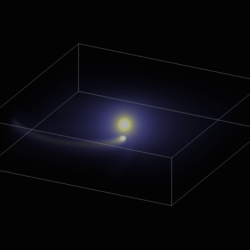
Figure 1: 3D rendering of the density of one of the models (C1b, see Table 2), after an integration time of $3.8\leavevmode\nobreak\ \mathrm{days}$.

The initial conditions are evolved for an integration time of $3.8\leavevmode\nobreak\ \mathrm{days}$, in which the planet completes an orbit around the star.

3 Results

As explored in previous works, the interaction between the stellar and planetary winds forms a wake structure similar to what is shown in Figure 1. The parameters we used for the wind sources result in similar morphology in all cases, where the morphological differences lie in the details. For instance, a rapid wind from the star results in a less curved and more radial wake than a slow wind, or a higher mass loss rate of the planet produces a larger bow-shock. Figure 2 shows the density stratification, temperature and ionizing heating rate for a cut in the orbital plane after an evolution time of $t=2.9\leavevmode\nobreak\ \mathrm{days}$.

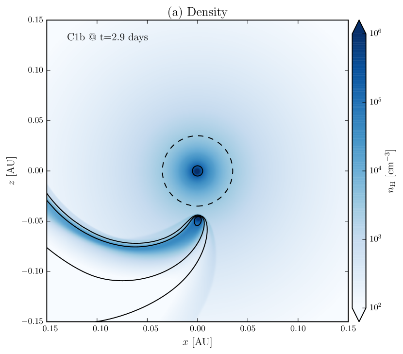
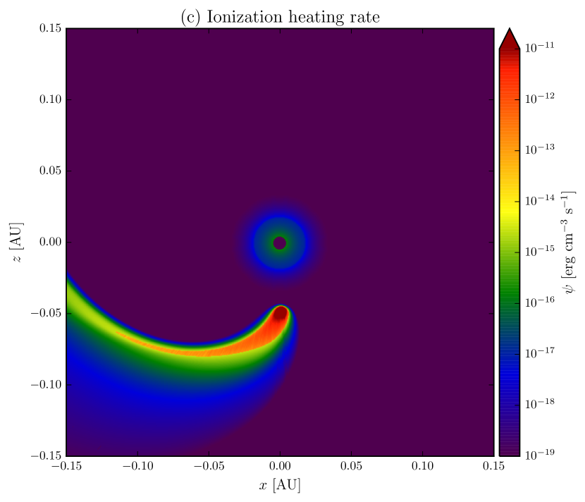
Figure 2: 2D cuts in the orbital plane ($y=0$) of (a) density, (b) temperature, and (c) ionization heating rate, at $t=2.9\leavevmode\nobreak\ \mathrm{days}$ for model C1b. In the top panel, we show the size of the central star (solid line circle) and the size of the region at which the wind is imposed (dashed line circle). In the same panel we also show ionization fraction iso-contours at values of $0.9$ (the most interior to the planet), $0.99$, and $0.999$ (the most exterior).

In the top panel we indicate by a solid circle the extent of HD 209458 (the photon packages are launched from this radius), and with a dashed circle the size of the region in which the stellar wind is imposed. In addition, the top panel of this Figure includes the ionization fraction isocontours at $0.9$ (close to the planet), $0.99$ and $0.999$ levels. The ionization structure of the tail is significantly different from our previous models, where the photoionization was not considered, and a fully neutral planetary wind was imposed. In Schneiter et al. (2007); Villarreal D’Angelo et al. (2014) we assumed that material arising from the planetary wind with a temperature $T<10^{5}\leavevmode\nobreak\ \mathrm{K}$ was neutral (and it was considered to estimate the Ly-$\alpha$ absorption). In the models with photoionization we now assume an ionization fraction of 0.8, which increases rapidly, implying that there is less material available to absorb.

From the other two panels, temperature and ionization heating rate stratification (b and c) it is clear how the impinging photons heat up the trailing planetary material and how the planet and the high density interaction region shield the outer part of escaping neutral atoms in the wake.

3.1 Ly-$\alpha$ absorption

To calculate the absorption produced by the escaping hydrogen we employed a similar post-processing procedure as in Schneiter et al. (2007) and Villarreal D’Angelo et al. (2014). For each of the simulations we compute the optical depth as a function of velocity along the LOS

$$\tau_{\mathrm{v_{los}}}=\int n_{\mathrm{HI}}\,a_{0}\,\varphi\left(\Delta v_{\mathrm{los}}\right)ds,$$ (8)

where $\varphi(\Delta v_{\mathrm{los}})$ is a Gaussian line-profile. The optical depth is obtained projecting the velocity on a LOS that is almost aligned with the $z$ and $-z$-axes, inclined $3.41\degr$ around the $x$-axis to have the same orientation as the HD 209548 system seen from Earth (an orbital inclination angle of $i=86.59\degr$). In the optical depth calculation we have considered a velocity range of $[-300,300]\leavevmode\nobreak\ \mathrm{km\leavevmode\nobreak\ s^{-1}}$, covered with $250$ velocity bins. By choosing the LOS close to $z$ and $-z$ we are able to observe two transits in the same orbit. The optical depth is only calculated considering the material on the observer’s side from the star.

The total absorption can be calculated by integrating $\tau_{\mathrm{v_{los}}}$ in velocity. The Ly-$\alpha$ emission from the star would be absorbed by a factor $(1-\mathrm{e}^{-\tau})$, where $\tau$ is the optical depth integrated over all velocities. Figure 3 shows an example (same model shown in Figures 1 and 2) of the total absorption fraction calculated from the models during a transit, as it would be seen by an observer in the $-z$ direction (with the inclination of HD 209458b).

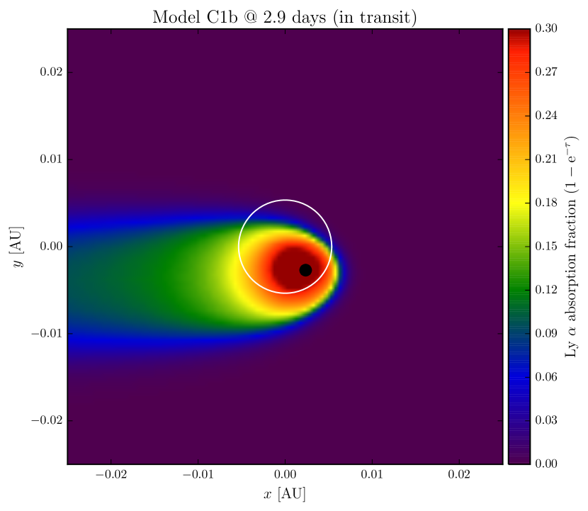
Figure 3: Map of Ly-$\alpha$ optical depth (integrated over all velocities) for model C1b in transit as observed from the $-z$-axis (integration time of $2.9\leavevmode\nobreak\ \mathrm{days}$). The map showed is zoom-in of the entire domain. Both the star and the planet are shown in scale by the white circle and black disk, respectively.

After computing the Ly-$\alpha$ absorption as a function of time, we found that the wake reaches a quasi-stationary state in only a fraction of the orbital period. This is somewhat different from our previous models, where at least half a period was required to reach such a stationary state. The main reason is that the photoionization results in a smaller neutral tail.

Figure 4 shows the absorption of the stellar emission as a function of time, first from the $+z$ direction ($t<2.2\leavevmode\nobreak\ \mathrm{days}$) and the subsequent transit as would be measured from the $-z$ direction (see Figure 2) for all the models.

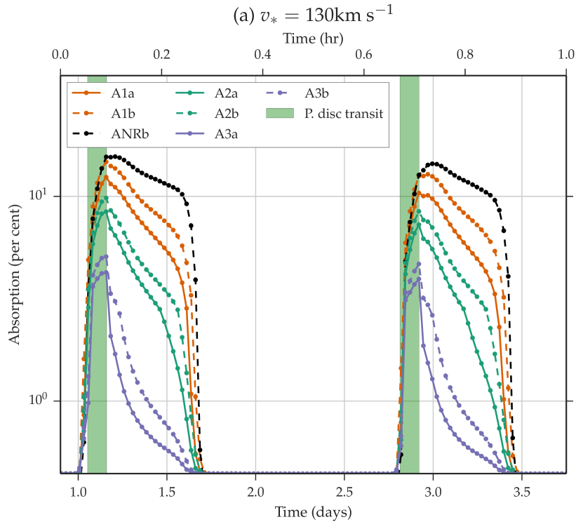
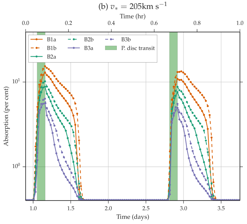
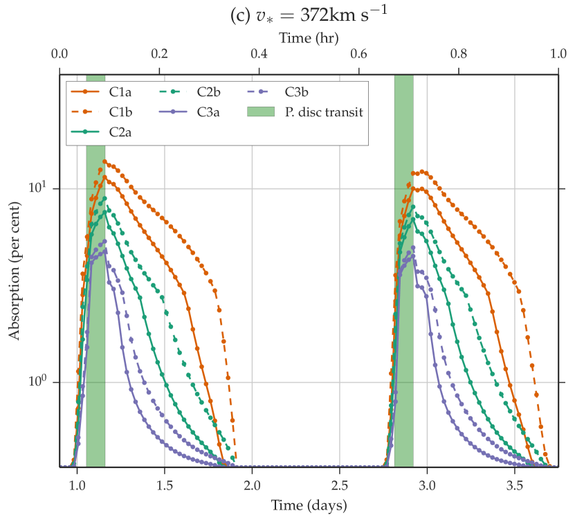
Figure 4: Velocity averaged total absorption as a function of time calculated from an observer situated in the +z (first transit $t<2.2\leavevmode\nobreak\ \mathrm{days}$) and -z directions (second transit, $t>2.2\leavevmode\nobreak\ \mathrm{days}$). The models are grouped into panels according to the stellar wind velocity, as indicated in the title. The color coding represents the ionizing flux: $0.2\leavevmode\nobreak\ S_{0}$ (orange), $S_{0}$ (green), and $5\leavevmode\nobreak\ S_{0}$ (purple). The dots joined by dotted lines correspond to $\dot{M}_{\mathrm{p}}=2\times 10^{10}\leavevmode\nobreak\ \mathrm{g\leavevmode\nobreak\ s^{-1}}$, and the solid lines to $\dot{M}_{\mathrm{p}}=1\times 10^{10}\leavevmode\nobreak\ \mathrm{g\leavevmode\nobreak\ s^{-1}}$. The green vertical stripe represents the times when a portion of the planetary disc blocks the star (i.e. the planet is in transit).

We have separated the models according to the stellar wind velocity. Panel (a) shows all the models with $v_{*}=130\leavevmode\nobreak\ \mathrm{km\leavevmode\nobreak\ s^{-1}}$, including the reference model ANRb that has the same parameters as A2b (see Table 2 for details) but does not include the photoionization process. In this model the absorption was computed as in (Schneiter et al., 2007), that is, assuming that only material originally from the planet with temperatures below $10^{5}\leavevmode\nobreak\ \mathrm{K}$ absorb the Ly-$\alpha$ emission. Panels (b) and (c) show the absorption for the models with $205$ and $372\leavevmode\nobreak\ \mathrm{km\leavevmode\nobreak\ s^{-1}}$, respectively. Notice that there are only minor differences in the first and second transits, showing that the quasi-stationary wake structure forms rapidly. The absorption in Figure 4 was calculated excluding the velocity range between $-40$ and $40\leavevmode\nobreak\ \mathrm{km\leavevmode\nobreak\ s^{-1}}$, which for Earth based observations is contaminated by the geocoronal emission.

From the plots we can see that the maximum absorption changes when doubling $\dot{M}_{p}$. This is in accordance with the results obtained in Schneiter et al. (2007)and Villarreal D’Angelo et al. (2014). At the same time the total absorption is greatly affected by the change in $F_{\mathrm{EUV}}$, producing appreciable changes both in the maximum absorption as well as in the tail of the wake (absorption after the transit of the planet), a denser and more extended structure is formed for low ionizing fluxes.

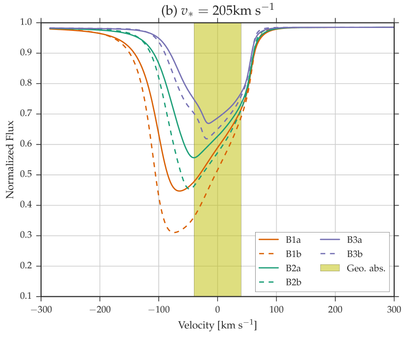
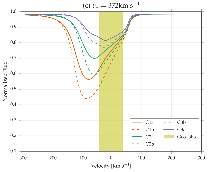
Figure 5: Normalized stellar emission at $t=2.9\leavevmode\nobreak\ \mathrm{days}$ as a function of LOS velocity. The models are grouped in the same manner as in Figure 4 Panel (a) includes the line profile for a simulations without radiation transfer (black line), calculated with the passive scalar and the a ionization temperature as in Schneiter et al. (2007); Villarreal D’Angelo et al. (2014). The yellow stripe represents the part of the line that is contaminated with the geocoronal glow and was omitted form the total absorption calculation.

From the detection made with the Space Telescope Imaging Spectrograph (STIS) on board of the Hubble Space Telescope (HST) in 2001 (see Vidal-Madjar et al., 2003) it is clear that the deepest absorption signatures are found in the blue wing of the Ly-$\alpha$ line, in the velocity range between $-130$ and $-40\leavevmode\nobreak\ \mathrm{km\leavevmode\nobreak\ s^{-1}}$. Whereas the red side of the Doppler Shifted absorption, defined within the velocity range between $32$ and $100\leavevmode\nobreak\ \mathrm{km\leavevmode\nobreak\ s^{-1}}$ is less significant. To study this features, we show in Figure 5 the stellar emission as a function of velocity, for all the models, at the time of maximum absorption during the second transit ($t=2.9\leavevmode\nobreak\ \mathrm{days}$).

From Figure 5 we notice that the absorption depends strongly on the ionizing flux, especially on the blue side of the spectrum, contrary to what it is observed on the red side, where all models show similar behaviour.

It is expected that higher ionizing fluxes result in a lower absorption, as photoionized material becomes transparent to Ly-$\alpha$. In addition, neutral material in the wake of the planetary wind accelerates due to its hydrodynamical interaction with the stellar wind, as well as due to radiation pressure (modeled here as a deficit in the gravitational pull of the star). The neutral wake therefore accelerates towards the observer (see Figure 2), and interacts with the Ly-$\alpha$ emission from the star producing the prominent blue-shifted absorption, whose maximum value shifts towards more negatives velocities when the ionizing flux diminish.

To compare our results with the observations we took the original off-transit data (reproduced from Vidal-Madjar et al., 2003), and multiplied them by the velocity dependent absorption factor in our models. The resulting Ly-$\alpha$ profiles can be compared with the in-transit observations in Figure 6 (also reproduced from Vidal-Madjar et al., 2003).

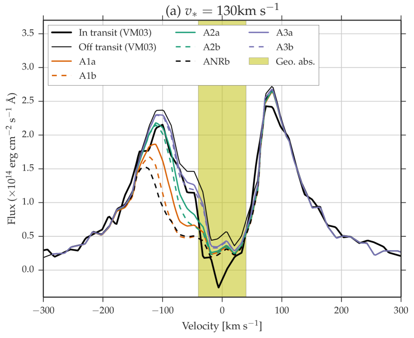
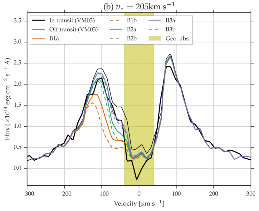
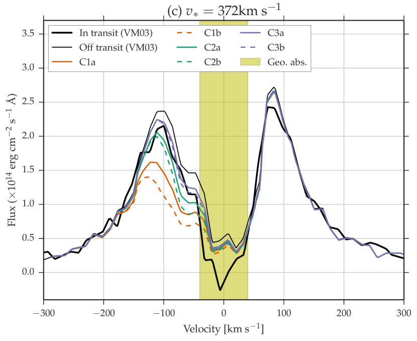
Figure 6: Ly-$\alpha$ observations (reproduced from Vidal-Madjar et al., 2003), and the corresponding synthetic absorption calculated with our models. The color and line coding is the same as in previous figures, and it is indicated in the label.

The observations show absorption in both the blue part of the spectrum (in the velocity range from $-130$ to $-40\leavevmode\nobreak\ \mathrm{km\leavevmode\nobreak\ s^{-1}}$), as well as in the red part of the spectrum (velocity range from $32$ to $100\leavevmode\nobreak\ \mathrm{km\leavevmode\nobreak\ s^{-1}}$) with an attenuation of $\sim 10\%$ and $\sim 5\%$, respectively.

Most of the models reproduce the level of absorption in the blue wing (except models with low stellar flux that overestimate the absorption for all velocities), considering the large uncertainties in the observations. The red wing absorption is generally underestimated, and only a couple of models show very little absorption around $90\leavevmode\nobreak\ \mathrm{km\leavevmode\nobreak\ s^{-1}}$.

In Figures 5 and 6 the region shaded in yellow corresponds to the part of the spectrum contaminated by geocoronal emission in observations, thus it should not be considered when comparing our models with observations.

4 Discussion

The models presented here are closer to a self-consistent study of the stellar-planetary wind interaction than the two previous works (Schneiter et al., 2007; Villarreal D’Angelo et al., 2014), where a proper photoionizating photon flux was not included.

Focusing on the the outer part of the planetary atmosphere ($r\gtrsim 3R_{\mathrm{p}}$), and adjusting the hydrodynamic parameters according the results in Schneiter et al. (2007); Villarreal D’Angelo et al. (2014), we have done a study of the influence of the high energy photon flux on the escaping part of the atmosphere. The maximum absorption is shown in Figure 4 (the portion shaded in green which corresponds to the planet transit), where a strong almost linear dependence on the high ionizing flux is found. The importance of the planetary mass loss rate becomes less obvious (almost negligible) within the accepted range estimated in previous works (Schneiter et al., 2007; Villarreal D’Angelo et al., 2014). At the same time, $\dot{M}_{\mathrm{p}}$ does affect the absorption in the tail (after the planetary transit). This result is not surprising, since most of the neutral material is swept, by the stellar wind, to produce the tail which, due to the orbital motion, and gravitational pull, it becomes curved getting exposed to the photoionizing flux incoming from the star (see Figures 1 and 2).

The stellar EUV flux in our models ranges between $\sim[1\times 10^{2}-4\times 10^{3}]$ erg $cm^{-2}$ $s^{-1}$. This implies that the planetary evaporation for HD 209458b will be driven by an energy limited mechanism (see Murray-Clay et al., 2009). Under this paradigm we can estimate the planetary mass loss rate from the simple equation (Yelle, 2004; Penz et al., 2008)

$$\dot{M}_{p}=\eta_{\mathrm{rad}}\frac{\pi R_{\mathrm{p}}^{3}F_{\mathrm{EUV}}}{GM_{\mathrm{p}}}$$ (9)

where $\eta_{rad}$ is the heating efficiency and $F_{\mathrm{EUV}}$ is the EUV flux at the position of the planet. $M_{\mathrm{p}}$, $R_{\mathrm{p}}$ are the mass and the planetary radius and $G$ is the gravitational constant. This formula does not take into account the correction for the Roche lobe effects that acording to Penz et al. (2008); Erkaev et al. (2007), can change the value of $\dot{M}_{\mathrm{p}}$ in a factor of $\sim 1.5$ for HD 209458b.
In our simulations, we fix the mass loss rate of the planet and the stellar flux for each model. This implies, according to the Eq. 9, to assume a certain value for the heating efficiency at the position where the planetary wind is launched. Hence, in our models, the heating efficiency varies from 2$\%$ to 100 $\%$. At the present, it is unclear what is the best value for $\eta$, but with our models we will be covering almost all possibles values. In the literature, several authors tried to constrain this factor: Tian et al. (2005) adopted a $\eta=0.6$ for a pure atomic H atmosphere, Ehrenreich & Désert (2011) obtained an $\eta>1$ based on the values of mass loss rate from Vidal-Madjar et al. (2003) and Linsky et al. (2010) and the luminosity value from Kashyap et al. (2008), Lammer et al. (2009) suggest $\eta\sim[10-25]\%$.
As a first aproximation, from Fig. 6, we can say that the lowest value of $F_{0}$ can’t reproduce the observed absorption, hence this models are not expected to be representative of the planetary system parameters. So, the highest values of $\eta$ ($\sim[50-100]\%$) are not expected to define the planetary atmosphere of HD 209458b.
It would be important to have some observational constraint to the value of $\eta$, as mentioned Ehrenreich & Désert (2011). This could shed some light into the atmospheric composition of exoplanets.

When comparing our models with the observations, in particular focusing on the Doppler blue-shifted part of the curve (Figure 6) we see that the $v_{*}=130\leavevmode\nobreak\ \mathrm{km\leavevmode\nobreak\ s^{-1}}$ peak is better fitted with the $S_{0}$ photon rate, whereas a lower absolute velocity part of the spectrum (between $-40$ to $-75\leavevmode\nobreak\ \mathrm{km\leavevmode\nobreak\ s^{-1}}$) is better fitted with a larger photon rate ($5\times S_{0}$) flux. The same trend is observed for larger wind velocity. Certainly with a more fine parameter coverage one could reproduce the absorption in more detail, however this is beyond the scope of this paper.

In a recent work, Tremblin & Chiang (2013) study the effect of charge exchange in the mixing region of the two winds. With their choice of parameters they are able to reproduce an asymmetric absorption (also favouring the blue wing), in particular the $\sim 10\%$ absorption at $-100\leavevmode\nobreak\ \mathrm{km\leavevmode\nobreak\ s^{-1}}$. Their parameters are similar to our model A1b, but with the inclusion of a treatment for charge exchange between the stellar and planetary winds.

In contrast to the studies of Tremblin & Chiang (2013); Holmström et al. (2008), our simulations did not inlude charge exchange but where still able to produce absorption at high blue Doppler-shift velocities, but due to the pure hydrodynamic interaction, along with the global radiation pressure. It is clear that both effects are expected to be present, and charge exchange in models as ours would enhance the absorption in the blue. An assessment of their relative (or collective) contribution is left for a follow up study.

The inclusion of the radiation transfer calculation also shows that the previous estimates of the planetary mass loss rates where a bit low. It is clear from Figure 4 that the same hydrodynamical parameters result in a overestimation of the absorption respect to the models that do include the photionization of the tail. Therefore, to reach a similar absorption with the photonionization included requires a larger mass loss rate. However the mass loss rates used in this work are compatible to previous estimates.

5 Conclusions

We used the 3D numerical hydrodynamic code Guacho, to simulate the interaction of the wind escaping a hot-Jupiter (with parameters resembling HD 209458b) and a photo-ionized wind coming from a solar-type star (HD 209458).

The ionizing flux was found to have a great influence on the neutral hydrogen escaping from the planet, producing an almost linear effect on the absorption of the wake. With planetary mass loss rates within the range proposed in Schneiter et al. (2007); Villarreal D’Angelo et al. (2014) it is possible to find EUV fluxes that reproduce the observed absorption measured in Vidal-Madjar et al. (2003) down to velocities less than $-100\leavevmode\nobreak\ \mathrm{km\leavevmode\nobreak\ s^{-1}}$. Perfoming 3D simulations that include the orbital motion of the planet is a natural way of obtaining a non-symmetric hydrogen envelop that is subject to the incoming stellar photons and wind.

Our models show that the hydrodynamic interaction between the planetary and stellar wind is able to reproduce the asymmetric absorption towards high blue-shifted velocities, as observed in (Vidal-Madjar et al., 2003). Such asymmetric absorption has been also attributed to charge-exchange between the fast stellar wind and the slow planetary wind (Tremblin & Chiang, 2013).

In a subsequent paper we plan to include the effects of the stellar magnetic fields together with the charge-exchange interaction. This will allow us to further constraint the photon flux and its influence on the acceleration of the neutral escaping material.

References

- Adams (2011) Adams F. C., 2011, ApJ, 730, 27
- Baraffe et al. (2005) Baraffe I., Chabrier G., Barman T. S., Selsis F., Allard F., Hauschildt P. H., 2005, aap, 436, L47
- Batygin & Stanley (2014) Batygin K., Stanley S., 2014, ApJ, 794, 10
- Ben-Jaffel (2007) Ben-Jaffel L., 2007, ApJL, 671, L61
- Ben-Jaffel (2008) Ben-Jaffel L., 2008, ApJ, 688, 1352