An efficient and portable SIMD algorithm for charge/current deposition in Particle-In-Cell codes

Abstract

In current computer architectures, data movement (from die to network) is by far the most energy consuming part of an algorithm (10pJ/word on-die to 10,000pJ/word on the network). To increase memory locality at the hardware level and reduce energy consumption related to data movement, future exascale computers tend to use more and more cores on each compute nodes ("fat nodes") that will have a reduced clock speed to allow for efficient cooling. To compensate for frequency decrease, machine vendors are making use of long SIMD instruction registers that are able to process multiple data with one arithmetic operator in one clock cycle. SIMD register length is expected to double every four years. As a consequence, Particle-In-Cell (PIC) codes will have to achieve good vectorization to fully take advantage of these upcoming architectures. In this paper, we present a new algorithm that allows for efficient and portable SIMD vectorization of current/charge deposition routines that are, along with the field gathering routines, among the most time consuming parts of the PIC algorithm. Our new algorithm uses a particular data structure that takes into account memory alignement constraints and avoids gather/scatter instructions that can significantly affect vectorization performances on current CPUs. The new algorithm was successfully implemented in the 3D skeleton PIC code PICSAR and tested on Haswell Xeon processors (AVX2-256 bits wide data registers). Results show a factor of $\times 2$ to $\times 2.5$ speed-up in double precision for particle shape factor of order $1$ to $3$. The new algorithm can be applied as is on future KNL (Knights Landing) architectures that will include AVX-512 instruction sets with 512 bits register lengths (8 doubles/16 singles).

1 Introduction

1.1 Challenges for porting PIC codes on exascale architectures: importance of vectorization

Achieving exascale computing facilities in the next decade will be a great challenge in terms of energy consumption and will imply hardware and software developments that directly impact our way of implementing PIC codes [1].

Operation	Energy cost	Year
DP FMADD flop	$11pJ$	2019
Cross-die per word access	$24pJ$	2019
DP DRAM read to register	$4800pJ$	2015
DP word transmit to neighbour	$7500pJ$	2015
DP word transmit across system	$9000pJ$	2015

Table 1: Energy consumption of different operations taken from [5]. The die hereby refers to the integrated circuit board made of semi-conductor materials that usually holds the functional units and fast memories (first levels of cache). This table shows the energy required to achieve different operations on current (Year 2015) and future (Year 2019) computer architectures. DP stands for Double Precision, FMADD for Fused Multiply ADD and DRAM for Dynamic Random Access Memory.

Table 1 shows the energy required to perform different operations ranging from arithmetic operations (fused multiply add or FMADD) to on-die memory/DRAM/Socket/Network memory accesses. As $1$pJ/flop/s is equivalent to $1$MW for exascale machines delivering $1$ exaflop ($10^{18}$ flops/sec), this simple table shows that as we go off the die, the cost of memory accesses and data movement becomes prohibitive and much more important than simple arithmetic operations. In addition to this energy limitation, the draconian reduction in power/flop and per byte will make data movement less reliable and more sensitive to noise, which also push towards an increase in data locality in our applications.

At the hardware level, part of this problem of memory locality was progressively adressed in the past few years by limiting costly network communications and grouping more computing ressources that share the same memory ("fat nodes"). However, partly due to cooling issues, grouping more and more of these computing units will imply a reduction of their clock speed. To compensate for the reduction of computing power due to clock speed, future CPUs will have much wider data registers that can process or "vectorize" multiple data in a single clock cycle (Single Instruction Multiple Data or SIMD).

At the software level, programmers will need to modify algorithms so that they achieve both memory locality and efficient vectorization to fully exploit the potential of future exascale computing architectures.

1.2 Need for portable vectorized routines

In a standard PIC code, the most time consuming routines are current/charge deposition from particles to the grid and field gathering from the grid to particles. These two operations usually account for more than $80\%$ of the execution time. Several portable deposition algorithms were developed and successfully implemented on past generations’ vector machines (e.g. CRAY, NEC) [9, 10, 11, 12, 13]. However, these algorithms do not give good performance on current SIMD architectures, that have new constraints in terms of memory alignement and data layout in memory.

To the authors’ knowledge, most of the vector deposition routines proposed in contemporary PIC codes use compiler based directives or even C++ Intel intrinsics in the particular case of the Intel compiler, to increase vectorization efficiency (e.g. [2]). However, these solutions are not portable and require code re-writing for each new architecture.

1.3 Paper outline

In this paper, we propose a portable algorithm for the direct deposition of current or charge from macro particles onto a grid, which gives good performances on SIMD machines. The paper is divided into four parts:

1. in section $2$, we quickly introduce the standalone 3D skeleton electromagnetic PIC code PICSAR-EM3D in which we implemented the different vector versions of the deposition routines presented in this paper,

2. in section $3$, we quickly remind the scalar deposition routine and show why it cannot be vectorized as is by the compiler. Then, we introduce a vector algorithm that performed well on former Cray vector machines but give poor performances on current SIMD machines. By carefully analyzing the bottlenecks of the old vector routine on current SIMD machines, we will derive a new vector routine that gives much better performances,

3. in section $4$ we present the new vector routines that was developed, based on the analysis in section $3$,

4. in section $5$, the new vector routines are benchmarked on the new Cori machine at the U.S. National Energy Research Supercomputer Center (NERSC) [8].

2 The PICSAR-EM3D PIC kernel

PICSAR-EM3D is a standalone "skeleton" PIC kernel written in Fortran 90 that was built using the main electromagnetic PIC routines (current deposition, particle pusher, field gathering, Yee field solver) of the framework WARP [7]. As WARP is a complex mix of Fortran 90, C and Python, PICSAR-EM3D provides an essential testbed for exploring PIC codes algorithms with multi-level parallelism for emerging and future exascale architectures. All the high performance carpentry and data structures in the code have been redesigned for best performance on emerging architectures, and tested on NERSC supercomputers (CRAY XC30 Edison and testbed with Intel Knight’s Corner coprocessors Babbage).

2.1 PIC algorithm

PICSAR-EM3D contains the essential features of the standard explicit electromagnetic PIC main loop:

1. Maxwell solver using arbitrary order finite-difference scheme (staggered or centered),

2. Field gathering routines including high-order particle shape factors (order 1 - CIC, order 2 - TSC and order 3 - QSP),

3. Boris particle pusher,

4. Most common types of current depositions : Morse-Nielson deposition [1] (also known as direct $\rho\textbf{v}$ current deposition) and Esirkepov [4] (charge conserving) schemes. The current and charge deposition routines support high-order particle shape factors (1 to 3).

2.2 High performance features

Many high performance features have already been included in PICSAR-EM3D. In the following, we give a quick overview of the main improvements that brought significant speed-up of the code and that are of interest for the remainder of this paper. A more comprehensive description of the code and its performances will be presented in another paper.

2.2.1 Particle tiling for memory locality

Field gathering (interpolation of field values from the grid to particle positions) and current/charge deposition (deposition of particle quantities to adjacent grid nodes) account for more than 80% of the total execution time of the code. In the deposition routines for instance, the code loops over all particles and deposit their charges/currents on the grid.

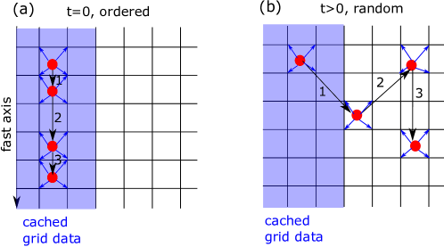
Figure 1: Importance of cache reuse in deposition routines. Illustration is given in 2D geometry for clarity, with CIC (linear) particle shapes. Panel (a) shows a typical layout at initialization (t=0) where particles are ordered along the "fast" axis of the grid, corresponding to grid cells (blue area) that are contiguous in memory. The loop on particles is illustrated with arrows and index of the loop with numbers 1 to 3. Using direct deposition, each particle (red point) deposits (blue arrows) its charge/current to the nearest vertices (4 in 2D and 8 in 3D for CIC particle shapes). Panel (b) illustrates the random case (at t>0) where particles are randomly distributed on the grid. As the algorithms loops over particles, it often requires access to uncached grid data, which then results in a substantial number of cache misses.

One major bottleneck that might arise in these routines and can significantly affect overall performance is cache reuse.

Indeed, at the beginning of the simulations (cf. Fig. 1 (a)) particles are typically ordered along the "fast" axis ("sorted case") that corresponds to parts of the grid that are contiguously located in memory. As the code loops over particles, it will thus access contiguous grid portions in memory from one particle to another and efficiently reuse cache.

However, as time evolves, the particle distribution often becomes increasingly random, leading to numerous cache misses in the deposition/gathering routines (cf. Fig. 1 (b)). This results in a considerable decrease in performance. In 2D geometry, one MPI subdomain usually fits in L2 cache (256kB to 512 kB per core) but for 3D problems with MPI subdomains handling 100x100x100 grid points, one MPI subdomain does not fit in cache anymore and random particle distribution of particles can lead to performance bottlenecks.

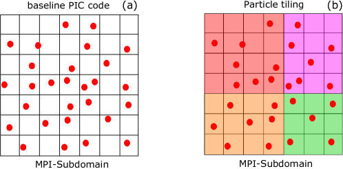
Figure 2: Particle tiling for efficient cache reuse. Panel (a) shows the usual configuration used in standard codes. There is one big array for particles for each MPI subdomain. Panel (b) shows the data structure used in PICSAR. Particles are grouped in tiles that fit in cache, allowing for efficient cache reuse during deposition/gathering routines.

To solve this problem and achieve good memory locality, we implemented particle tiling in PICSAR-EM3D. Particles are placed in tiles that fit in cache (cf. Fig. 1 (b)). In the code, a tile is represented by a structure of array Type(particle_tile) that contains arrays of particle quantities (positions, velocity and weight). All the tiles are represented by a 3D Fortran array array_of_tiles(:,:,:) of type particle_tile in the code. Our data structure is thus very different from the one in [3] which uses one large Fortran $ppart(1:ndims,1:nppmax,1:ntiles)$ array for all particles and tiles, where $ndims$ is the number of particle attributes (e.g positions $x$, $y$, $z$), $nppmax$ the maximum number of particles in a tile and $ntiles$ the number of tiles. There are two reasons behind our choice:

1. if one tile has much more particles than others, we considerably save memory by using our derived type compared to the array $ppart$. Indeed, in the latter case, if one tile has much more particles $np$ than others, we would still need to choose $nppmax\geqslant np$ for all the tiles,

2. any tile can be resized as needed independently, without the need for reallocating the entire array of tiles.

Performance improvements of the whole code are reported on table 2 for tests performed on Intel Ivy Bridge (Cray XC30 Edison machine at NERSC). These tests show a speed-up of x3 in case of a random particle distribution. Cache reuse using tiling reaches $99\%$. The optimal tile size ranges empirically between 8x8x8 cells to 10x10x10 cells. As will be shown later in the paper, having good cache reuse is crucial to increasing the flop/byte ratio of the proposed algorithm and obtaining improvements using vectorization.

Tile size	Speed-up	L1 and L2 Cache reuse
$1\times 1\times 1$	$\times 1$	$85\%$
$10\times 10\times 10$	$\times 3$	$99\%$

Table 2: Speed-up of the whole PIC code brought by particle tiling. Tests were performed using a 100x100x100 grid with 10 particle per cells. Particles are randomly distributed on the grid and have an initial temperature of $10keV$. The reference time corresponds to the standard case of 1x1x1 tile. The tests were performed on one MPI process and a single socket, on the Edison cluster at NERSC.

Notice that at each time step, the particles of each tile are advanced and then exchanged between tiles. As particles move less than one cell at each time step, the amount of particles exchanged between tiles at each time step is low for typical tiles’ sizes. (The surface/volume ratio decreases with tile size.) As a consequence, particle exchanges between tiles account in practice for a very small percentage of the total PIC loop (a few percents). Our particle exchange algorithm differs from the one used in [3] in that it avoids copying data into buffers. In addition, it can be efficiently parallelized using OpenMP (details are beyond the scope for this paper and will be presented in an upcoming publication).

2.2.2 Multi-level parallelization

PICSAR-EM3D also includes the following high performance implementations:

1. vectorization of deposition and gathering routines,

2. OpenMP parallelization for intranode parallelisms. Each OpenMP thread handles one tile. As there are much more tiles than threads in 3D, load balancing can be easily done using the SCHEDULE clause in openMP with the guided attribute,

3. MPI parallelization for internode parallelism,

4. MPI communications are overlapped with computations. For particles, this is done by treating exchanges of particles with border tiles while performing computations on particles in inner tiles,

5. MPI-IO for fast parallel outputs.

In the remainder of this paper, we will focus on the vectorization of direct charge/current deposition routines for their simplicity and widespread use in electromagnetic PIC codes. The Esirkepov-like current deposition is not treated in this paper but the techniques used here are very general and should apply in principle to any kind of current deposition.

3 Former CRAY vector algorithms and performance challenges on new architectures

In the following, we focus on the direct $3D$ charge deposition which can be presented in a more concise way than the full $3D$ current deposition. Vectorization methods presented for charge deposition can easily be transposed to current deposition and $3D$ vector algorithms for current deposition can be found in appendix B.

3.1 Scalar algorithm

The scalar algorithm for order 1 charge deposition is detailed in listing 1. For each particle index $ip$, this algorithm (see line $5$):

1. finds the indices $(j,k,l)$ of the cell containing the particle (lines $11-13$),

2. computes the weights of the particle at the 8 nearest vertices $w1$ to $w8$ (line $15$-not shown here),

3. adds charge contribution to the eight nearest vertices $\{(j,k,l),(j+1,k,l),(j,k+1,l),(j+1,k+1,l),(j,k,l+1),(j+1,k,l+1),(j,k+1,l+1),(j+1,k+1,l+1)\}$ of the current cell $(j,k,l)$ (see lines $18-25$).

Listing 1: Scalar charge deposition routine for CIC particle shape factors

⬇

1SUBROUTINE depose_rho_scalar_1_1_1(...)

2 ! Declaration and init

3 ! ...........7

4 ! Loop on particles

5 DO ip=1,np

6 ! --- computes current position in grid units

7 x = (xp(ip)-xmin)*dxi

8 y = (yp(ip)-ymin)*dyi

9 z = (zp(ip)-zmin)*dzi

10 ! --- finds node of cell containing particle

11 j=floor(x)

12 k=floor(y)

13 l=floor(z)

14 ! --- computes weigths w1..w8

15 ........

16 ! --- add charge density contributions

17 ! --- to the 8 vertices of current cell

18 rho(j,k,l) =rho(j,k,l) + w1

19 rho(j+1,k,l) =rho(j+1,k,l) + w2

20 rho(j,k+1,l) =rho(j,k+1,l) + w3

21 rho(j+1,k+1,l) =rho(j+1,k+1,l) + w4

22 rho(j,k,l+1) =rho(j,k,l+1) + w5

23 rho(j+1,k,l+1) =rho(j+1,k,l+1) + w6

24 rho(j,k+1,l+1) =rho(j,k+1,l+1) + w7

25 rho(j+1,k+1,l+1) =rho(j+1,k+1,l+1)+ w8

26 END DO

27END SUBROUTINE depose_rho_scalar_1_1_1

As two different particles $ip_{1}$ and $ip_{2}$ can contribute to the charge at the same grid nodes, the loop over particles (line $5$) presents a dependency and is thus not vectorizable as is.

3.2 Former vector algorithms and new architecture constraints

Several vector algorithms have already been derived and tuned on former Cray vector machines [9, 10, 11, 12, 13, 14]. However, these techniques are not adapted anymore to current architectures and yield very poor results on SIMD machines that necessitate to comply with the three following constraints in order to enable vector performances:

1. Good cache reuse. The flop/byte ratio (i.e. cache reuse) in the main loops of the PIC algorithm must be high in order to observe a speed-up with vectorization. Otherwise, if data has to be moved from memory to caches frequently, the performance gain with vectorization can become obscured by the cost of data movement. As we showed earlier, this is ensured by particle tiling in our code,

2. Memory alignement. Data structures in the code need to be aligned and accessed in a contiguous fashion in order to maximize performances. Modern computers read from or write to a memory address in word-sized chunks of 8 bytes (for 64 bit systems). Data alignment consists in putting the data at a memory address equal to some multiple of the word size, which increases the system’s performance due to the way the CPU handles memory. SSE2, AVX and AVX-512 on x86 CPUs do require the data to be 128-bits, 256-bits and 512-bits aligned respectively, and there can be substantial performance advantages from using aligned data on these architectures. Moreover, compilers can generate more optimal vector code when data is known to be aligned in memory. In practice, the compiler can enforce data alignment at given memory boundaries (128, 256 or 512 bits) using compiler flags/directives.

3. Unit-stride read/write. If data are accessed contiguously in a do loop (unit-stride), the compiler will generate vector single load/store instructions for the data to be processed. Otherwise, if data are accessed randomly or via indirect indexing, the compiler might generate gather/scatter instructions that almost yield sequential performance or worse. Indeed, in case of a gather/scatter, the processor might have to make several different loads/stores from/to memory instead of one load/store, eventually leading to poor vector performances.

In the following, we investigate performances of one of the former vector algorithm for CRAY machines [11] and analyze its bottlenecks on SIMD architectures. This analysis will show a way to improve the vector algorithm and derive a new one that yields significant speed-up over the scalar version.

3.3 Example: the Schwarzmeier and Hewit scheme (SH)

3.3.1 SH vector deposition routine

Listing 2 details the Schwarzmeier and Hewitt (SH) deposition scheme [11] that was implemented in PICSAR-EM3D and tested on Cori supercomputer at NERSC. In this scheme, the initial loop on particles is done by blocks of lengths $nblk$ (cf. line $5$) and split in two consecutive nested loops:

• A first nested loop (line $7$) that computes, for each particle $nn$ of the current block:

  1. its cell position $ind0$ on the mesh (line $13$),

  2. its contribution $ww(1,nn),...,ww(8,nn)$ to the charge at the $8$ vertices of the cell and

  3. the indices $ll(1,nn),...,ll(8,nn)$ of the $8$ nearest vertices in the 1D density array rho (cf. lines $14-19$).

  Notice that 1D indexing is now used for $rho$ to avoid storing three different indices for each one of the 8 vertices. The Fortran integer array $moff(1:8)$ gives the indices of the 8 vertices with respect to the cell index $ind0$ in the 1D array $rho$. The loop at line $7$ has no dependencies and is vectorized using the portable $OMP SIMD directive.

• A second nested loop (line $23$) that adds the contribution of each one of the $nblk$ particles to the $8$ nearest vertices of their cell (line $26$). As one particle adds its contribution to eight different vertices, the loop on the vertices at line $25$ has no dependency and can also be vectorized using the $OMP SIMD directive.

Usually, $nblk$ is chosen as a multiple of the vector length. Notice that using a moderate size $nblk$, for the blocks of particles, ensures that the temporary arrays $ww$ and $ll$ fit in cache.

The SH algorithm presented on listing 2 is fully vectorizable and gave very good performances on former Cray machines [11, 13]. However as we show in the following section, it yields very poor performances on SIMD architectures.

Listing 2: Vector version of the charge deposition routine developed by SH for CIC particle shape factors

⬇

1SUBROUTINE depose_rho_vecSH_1_1_1(...)

2 ! Declaration and init

3 .....

4 ! Loop on particles

5 DO ip=1,np,nblk

6 !$OMP SIMD

7 DO n=ip,MIN(ip+nblk-1,np) !!!! VECTOR

8 nn=n-ip+1

9 !- Computations relative to particle ip (cell position etc.)

10 ...

11 ! --- computes weight for each of the 8-vertices of the current cell

12 ! --- computes indices of 8-vertices in the array rho

13 ind0 = (j+nxguard+1) + (k+nyguard+1)*nnx + (l+nzguard+1)*nnxy

14 ww(1,nn) = sx0*sy0*sz0*wq

15 ll(1,nn) = ind0+moff(1)

16 ...

17 ...

18 ww(8,nn) = sx1*sy1*sz1*wq

19 ll(8,nn) = ind0+moff(8)

20 END DO

21 !$OMP END SIMD

22 ! --- add charge density contributions

23 DO m= 1,MIN(nblk,np-ip+1)

24 !$OMP SIMD

25 DO l=1,8 !!!! VECTOR

26 rho(ll(l,m)) = rho(ll(l,m))+ww(l,m)

27 END DO

28 !$OMP END SIMD

29 END DO

30 END DO

31 ...

32END SUBROUTINE depose_rho_vecSH_1_1_1

3.3.2 Tests of the Schwarzmeier and Hewit algorithm on Cori

The SH algorithm was tested on one socket of the Cori cluster at NERSC. This socket had one Haswell Xeon processor with the following characteristics:

1. 16-core CPU at 2.3 GHz,

2. 256-bit wide vector unit registers (4 doubles, 8 singles) with AVX2 support,

3. 256kB L2 cache/core, 40MB shared L3 cache.

The Intel compiler was used to compile the code with option "-O3". The simulation was ran using 1 MPI process and 1 OpenMP thread per MPI process, with the following numerical parameters:

1. $100\times 100\times 100$ grid points with $10\times 10\times 10=1000$ tiles i.e $10$ tiles in each direction,

2. Two particle species (proton and electron) with 10 particle per cells. The particles are randomly distributed across the simulation domain. The plasma has an initial temperature of $10$ keV.

The results are displayed on table 3 for order 1 scalar and SH routines, using two different compiler options in each case:

1. -xCORE-AVX2 to enable vectorization,

2. -no-vec to disable auto-vectorization of the compiler. In this case, we also manually remove !$OMP SIMD directives to avoid simd vectorization of loops.

Routine	depose_rho_scalar_1_1_1		depose_rho_vecSH_1_1_1
Compiler option	-no-vec	-xCORE-AVX2	-no-vec	-xCORE-AVX2
Time/it/part	$14.6ns$	$14.6ns$	$21ns$	$15.9ns$

Table 3: Performance comparisons of scalar and SH vector routines.

The scalar routine takes the same time for -xCORE-AVX2 and -no-vec options because the routine is not auto-vectorizable by the compiler.

For the vector routine, we see an improvement of $30\%$ between -xCORE-AVX2 and -no-vec options, showing that vectorization is enabled and working in the -xCORE-AVX2 case. Nevertheless, the overall performance is poor, and the vector routine compiled with -xCORE-AVX2 is even $10\%$ slower than the scalar routine.

By looking at the code on listing 2 and using compiler report/ assembly code generated by the Intel compiler, we found two main reasons for this poor performance:

1. The first one comes from the strided access of the arrays $ww$ and $ll$ in the loop at line $7$. Assuming cache line sizes of $64$ bytes (8 doubles) and 256-bits wide registers, the four different elements $ww(1,nn_{1})$ to $ww(1,nn_{1}+3)$ are thus on four different cache lines ($ww$ is of size (8,$nblk$)) and this strided access necessitates $4$ stores in memory at different cache lines ("scatter") instead of a single store if the accesses were aligned and contiguous. A solution would be to switch dimensions of $ww$ but this might not bring any improvement at all because the loop on vertices (line $25$) would then have strided access for $ww$ ("gather"). Some PIC implementations choose contiguous access for $ww$/$ll$ in the first loop and then use an efficient vector transpose of $ww$/$ll$ before the second loop on vertices. However, this solution requires the use of "shuffle" Intel vector intrinsics to efficiently implement the transpose, which is not portable because this transpose will have to be re-written for a different processor. In addition, this transpose is done $8\times np$ with $np$ the number of particles and might thus add a non-negligible overhead if not done properly.

2. The second bottleneck comes from the indirect indexing for $rho$ at line $26$. The problem with the current data structure of $rho$ is that the $8$ vertices of one cell are not contiguous in memory, resulting in a rather inefficient gather/scatter instruction.

In the next section, we propose a portable solution for order $1$, $2$ and $3$ charge deposition that solves these two problems and yields a speed-up factor of up to $\times 2.5$ in double precision over the scalar routine.

4 New and portable SIMD algorithms

In this section, we present vector algorithms that perform efficiently on SIMD architectures.

4.1 CIC (order $1$) particle shape

4.1.1 Algorithm

The new vector algorithm is detailed on listing 3. Similarly to the SH routine, the main particle loop is done by blocks of $nblk$ particles and divided in two consecutive nested loops: $(i)$ a first nested loop that computes particle weights and $(ii)$ a second one that adds the particle weights to its $8$ nearest vertices.

4.1.2 Improvements brought by the new algorithm

The new algorithm adresses the two main bottlenecks of the SH algorithm with the two following new features:

1. a new data structure for $rho$ is introduced, named $rhocells$, which enables memory alignement and unit-stride access when depositing charge on the $8$ vertices. In $rhocells$, the 8-nearest vertices are stored contiguously for each cell. The array $rhocells$ is thus of size $(8,NCELLS)$ with $NCELLS$ the total number of cells. The element $rhocells(1,icell)$ is therefore 64 bytes-memory aligned for a given cell $icell$ and the elements $rhocells(1:8,icell)$ entirely fit in one cache line allowing for efficient vector load/stores. The array $rhocells$ is reduced to $rho$ once, after the deposition is done for all particles (cf. line $46$). This step is easily vectorizable (see line $48$) but might not lead to optimal performances due to the non-contiguous access in $rho$ that leads to gather-scatter instructions. Notice however that this time, this operation is proportional to the number of cells $NCELLS$ and not to the number of particles $np$ as it was in the case of the SH algorithm. The overhead is thus proportionally lower when there are more particles than cells, which is the case in many PIC simulations of interest,

2. for each particle, the $8$ different weights $ww$ are now computed using a generic formula (see line $39$) that suppresses gather instructions formerly needed in the SH algorithm. This also avoids implementing non-portable efficient transpose between the first and second loop, rendering this new algorithm fully portable.

Listing 3: New vector version of charge deposition routine for CIC (order $1$) particle shape factor

⬇

1 SUBROUTINE depose_rho_vecHVv2_1_1_1(...)

2 ! Declaration and init

3 ...

4 nnx = ngridx; nnxy = nnx*ngridy

5 moff = (/0,1,nnx,nnx+1,nnxy,nnxy+1,nnxy+nnx,nnxy+nnx+1/)

6 mx=(/1_num,0_num,1_num,0_num,1_num,0_num,1_num,0_num/)

7 my=(/1_num,1_num,0_num,0_num,1_num,1_num,0_num,0_num/)

8 mz=(/1_num,1_num,1_num,1_num,0_num,0_num,0_num,0_num/)

9 sgn=(/-1_num,1_num,1_num,-1_num,1_num,-1_num,-1_num,1_num/)

10

11 ! FIRST LOOP: computes cell index of particle and their weight on vertices

12 DO ip=1,np,LVEC

13 !$OMP SIMD

14 DO n=1,MIN(LVEC,np-ip+1)

15 nn=ip+n-1

16 ! Calculation relative to particle n

17 ! --- computes current position in grid units

18 x= (xp(nn)-xmin)*dxi

19 y = (yp(nn)-ymin)*dyi

20 z = (zp(nn)-zmin)*dzi

21 ! --- finds cell containing particles for current positions

22 j=floor(x)

23 k=floor(y)

24 l=floor(z)

25 ICELL(n)=1+j+nxguard+(k+nyguard+1)*(nx+2*nxguard) &

26 +(l+nzguard+1)*(ny+2*nyguard)

27 ! --- computes distance between particle and node for current positions

28 sx(n) = x-j

29 sy(n) = y-k

30 sz(n) = z-l

31 ! --- computes particles weights

32 wq(n)=q*w(nn)*invvol

33 END DO

34 !$OMP END SIMD

35 ! Charge deposition on vertices

36 DO n=1,MIN(LVEC,np-ip+1)

37 ! --- add charge density contributions to vertices of the current cell

38 ic=ICELL(n)

39 !$OMP SIMD

40 DO nv=1,8 !!! - VECTOR

41 ww=(-mx(nv)+sx(n))*(-my(nv)+sy(n))* &

42 (-mz(nv)+sz(n))*wq(n)*sgn(nv)

43 rhocells(nv,ic)=rhocells(nv,ic)+ww

44 END DO

45 !$OMP END SIMD

46 END DO

47 END DO

48 ! - reduction of rhocells in rho

49 DO iz=1, ncz

50 DO iy=1,ncy

51 !$OMP SIMD

52 DO ix=1,ncx !! VECTOR (take ncx multiple of vector length)

53 ic=ix+(iy-1)*ncx+(iz-1)*ncxy

54 igrid=ic+(iy-1)*ngx+(iz-1)*ngxy

55 rho(orig+igrid+moff(1))=rho(orig+igrid+moff(1))+rhocells(1,ic)

56 rho(orig+igrid+moff(2))=rho(orig+igrid+moff(2))+rhocells(2,ic)

57 rho(orig+igrid+moff(3))=rho(orig+igrid+moff(3))+rhocells(3,ic)

58 rho(orig+igrid+moff(4))=rho(orig+igrid+moff(4))+rhocells(4,ic)

59 rho(orig+igrid+moff(5))=rho(orig+igrid+moff(5))+rhocells(5,ic)

60 rho(orig+igrid+moff(6))=rho(orig+igrid+moff(6))+rhocells(6,ic)

61 rho(orig+igrid+moff(7))=rho(orig+igrid+moff(7))+rhocells(7,ic)

62 rho(orig+igrid+moff(8))=rho(orig+igrid+moff(8))+rhocells(8,ic)

63 END DO

64 !$OMP END SIMD

65 END DO

66 END DO

67

68 ...

69 END SUBROUTINE depose_rho_vecHVv2_1_1_1

4.2 Higher particle shape factors

Similar algorithms were derived for order $2$ (TSC) and order $3$ particle shape factors, and are detailed in Appendix A. Corresponding current deposition algorithms can be found in Appendix B for orders $1$, $2$ and $3$ depositions. In these algorithms (see Appenfix B), we use three structures $jxcells$, $jycells$ and $jzcells$ (analogous to $rhocells$ for the deposition of $rho$) for the current components $jx$, $jy$, $jz$ along directions $x$, $y$ and $z$.

In the following, we detail the data structures used for $rhocells$ for orders $2$ and $3$ particle shapes (cf. Fig. 3):

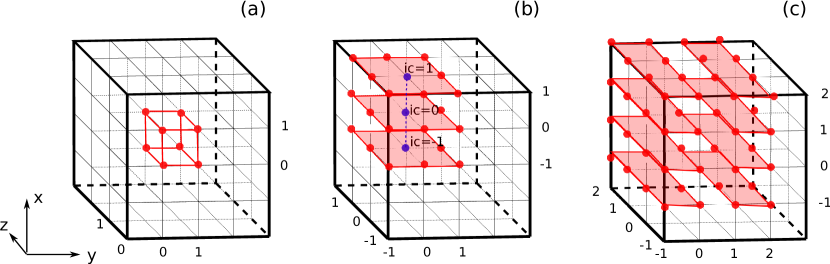
Figure 3: Data structure used for the array $rhocells$ for different particle shape factors. In each plot, the particle that deposits charge to its nearest vertices (red/blue points) is located in the cell at position (0,0,0). (a) CIC (order $1$) particle shape factor. The particle deposits its charge to the eight nearest vertices (red points). For each cell $icell=(j,k,l)$, $rhocells$ stores the $8$ nearest vertices $(j,k,l)$, $(j+1,k,l)$, $(j,k+1,l)$, $(j+1,k+1,l)$, $(j,k,l+1)$, $(j+1,k,l+1)$, $(j,k+1,l+1)$ and $(j+1,k+1,l+1)$ contiguously. (b) TSC (order $2$) particle shape factor. The particle deposits its charge to the $27$ neighboring vertices (red and blue points). For a given cell $icell=(j,k,l)$ $rhocells$ stores contiguously the $8$ vertices (red points) $(j,k-1,l-1)$, $(j,k,l-1)$, $(j,k+1,l-1)$, $(j,k-1,l)$, $(j,k+1,l)$, $(j,k-1,l+1)$, $(j,k,l+1)$ and $(j,k+1,l+1)$. The blue points are not stored in rhocells and are treated scalarly in the algorithm. (c) QSP (order $3$) particle shape factor. The particle deposits its charge to the $64$ neighboring vertices (red points). For a given cell $icell=(j,k,l)$, $rhocells$ stores contiguously the $8$ vertices (delimited by red areas) $(j,k-1,l-1)$, $(j,k,l-1)$, $(j,k+1,l-1)$, $(j,k+1,l-1)$, $(j,k-1,l)$, $(j,k,l)$, $(j,k+1,l)$, $(j,k+1,l)$ .

1. TSC (order $2$) particle shape. (cf. panel(b) of Fig. 3 and listing 5 in appendix A). In this case, the particles deposit their charge to the $27$ neighbouring vertices. However, storing $27$ contiguous vertices per cell in $rhocells$ would not be efficient as the reduction of $rhocells$ to $rho$ would be much more expensive with potential cache-reuse inefficiency. Instead, while the same size for $rhocells(1:8,1:NCELLS)$ is used, the vertices are now grouped in a different way. The new structure for $rhocells(1:8,1:NCELLS)$ groups $8$ points in a $(y,z)$ plane for each cell $icell$ (see red points in red areas). For each cell, each particle adds its charge contribution to 24 points in the three planes at $icell-1$, $icell$ and $icell+1$. The three remaining central points (blue points) can be either treated scalarly for $512$-bits wide vector registers or vectorized for $256$-bits by artificially adding a virtual point that does not contribute to any charge. Notice that we did not find a generic formulation for the weights $ww$ and we are therefore still performing a "gather" instruction for $ww$ in the loop on the vertice (line $101$ on listing 5). However, this gather is performed in the $y$ and $z$ directions for the first plane of $8$ points (plane $ic=-1$ on panel (b)) and is subsequently reused on the two other planes $ic=0$ and $ic=1$ (see lines $103$ to $107$ on listing 5). Gather is thus performed only 8 times out of 24 points and thus has a limited impact on performance, as shown below in the reported test results.

2. QSP (order $3$) particle shape. (cf. panel(c) of Fig. 3 and listing 6 in appendix A). In this case, particles deposit their charge to the $64$ neighbouring vertices. $rhocells(1:8,1:NCELLS)$ also group $8$ points in a ($y$,$z$) plane but differently from the TSC case (see red areas in panel (c)). For each cell, each particle adds its charge contribution to 64 points in the 8 different $(y,z)$ planes at $icell-ncx-1$, $icell-ncx$, $icell-ncx+1$, $icell-ncx+2$, $icell+ncx-1$,$icell+ncx$,$icell+ncx+1$ and $icell+ncx+2$ where $ncx$ is the number of cells in the $x$ direction (see lines $63$ to $77$ on listing 6). This might reduce the flop/byte ratio of the second loop when $nnx$ is large enough so that elements $rhocells(1:8,icell)$ and $rhocells(1:8,icell+nnx-1)$ are not in $L1$ cache. The vertices could have been grouped in $(y,z)$ planes of $16$ points instead of $8$ points but this would imply a bigger reduction loop of $rhocells$ in $rho$ and worst performances for a low number of particles. Notice that here again, we did not find an efficient generic formulation for the weights $ww$ and we are therefore still performing a "gather" instruction (see lines $116$ and $126$ on listing 6). However, this gather is performed in the $y$ and $z$ directions and is subsequently for computing the weights at different positions in $x$ (see lines $118$ to $124$ and $128$ to $134$ on listing 6). Gather is thus performed only 16 times out of 64 points and thus has a limited impact on performance, as shown below in the reported test results.

5 Benchmarks of the new algorithms

The new vector algorithms were benchmarked on one node (two sockets) of the Cori machine in the same numerical conditions than the ones used in section 3.3.2 but with 2 MPI processes (one per socket) and 16 OpenMP threads per MPI process. For charge deposition, we use 10x10x10 tiles in each direction. For current deposition, we use a larger number of tiles (12x12x12 tiles in each direction) so that the three structures $jxcells$, $jycells$ and $jzcells$ (equivalent of $rhocells$ for current deposition) fit in cache. Results are shown on Fig. 4 for charge deposition and on Fig. 5 for current deposition. Panels (a) show the time/iteration/particle (in $ps$ for Fig. 4 and ns for Fig. 5 ) taken by the deposition routines for different particle shape factors and when there are $10$ times more particles than cells. Panels (b) show the same quantities but for $40$ times more particles than cells.

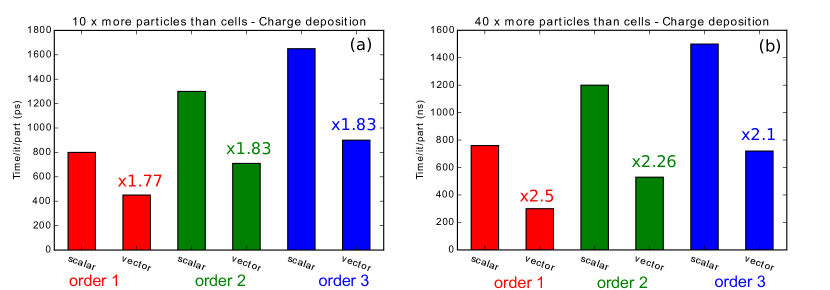
Figure 4: Benchmarks of the new $3D$ charge deposition algorithms on Cori. Each bar plot shows the time/it/part in $ps$ for different particle shape orders $1$ to $3$. (a) Benchmarks with $10$ times more particles than cells. (b) Benchmarks with $40$ times more particles than cells.

Notice that as we vectorize on vertices, there is no performance bottleneck related to a possibly inhomogeneous distribution of particles on the simulation domain. Even for a low number of particles per cell (e.g panel (a) of Fig. 4), the algorithm performs well, with speed-ups of up to $\times 1.8$. When the number of particles increases (Fig. 4 of panel (b)) performances are even better because the reduction operation of $rhocells$ in $rho$ becomes more and more negligible relatively to particle loops. For $40$ times more particles than cells, performances now reach $\times 2.5$ for order $1$ particle shape factor. Order $3$ deposition performs less efficiently than orders $1$ and $2$, because as we described in the previous section, the structure we chose for $rhocells$ decreases the flop/byte ratio of the loop on vertices compared to orders $1$ and $2$. In the case of simulations using a lot of particles, for which the reduction of $rhocells$ in $rho$ is negligible, one might consider grouping vertices in $rhocells$ by groups of $16$ instead of $8$ for order $3$ deposition in order to increase the flop/byte ratio in loop on vertices.

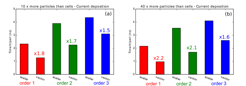
Figure 5: Benchmarks of the new $3D$ current deposition algorithms on Cori. Each bar plot shows the time/it/part in $ns$ for different particle shape orders $1$ to $3$. (a) Benchmarks with $10$ times more particles than cells. (b) Benchmarks with $40$ times more particles than cells.

6 Conclusion and prospects

A new method is presented that allows for efficient vectorization of the standard charge/current deposition routines on current SIMD architectures, leading to efficient deposition algorithms for shape factors of order 1, 2 and 3. The algorithms can be used on current multi-core architectures (with up to AVX2 support) as well as on future many-core Intel $KNL$ processors that will support $AVX-512$. Further tests on KNL will be performed as the processor becomes available.

This work provides deposition routines that are fully portable and only use the $OMP SIMD directives that are provided by OpenMP $4.0$. Efficient vectorization of the charge conserving current deposition from Esirkepov is being investigated, and will be detailed in future work.

Appendix A Full vector algorithms in Fortran 90 for order $1$, $2$ and $3$ charge deposition routines

In the following we use the notations below for input/output parameters of charge deposition subroutines:

• $rho$ is the charge density (grid array),

• $np$ is the number of particles (scalar),

• $xp,yp,zp$ are particle positions (particle arrays)

• $w$ is the particle weights (particle array) and $q$ the particle species charge (scalar)

• $xmin,ymin,zmin$ are the absolute coordinates (scalars) of the origin of the current spatial partition (tile or MPI subdomain depending on implementation) containing particle arrays (tile or subdomain),

• $dx,dy,dz$ (scalars) are the spatial mesh size in each direction,

• $nx,ny,nz$ (scalars) are the number of cells in each direction (without guard cells) of the current spatial partition,

• $nxguard,nyguard,nzguard$ (scalars) are the number of guard cells in each direction of the current spatial partition.

A.1 Order $1$ charge deposition routine

Listing 4: New vector version of charge deposition routine for CIC particle shape factors

⬇

1 SUBROUTINE depose_rho_vecHVv2_1_1_1(rho,np,xp,yp,zp,w,q,xmin,ymin,zmin, &

2 dx,dy,dz,nx,ny,nz,nxguard,nyguard,nzguard)

3 USE constants

4 IMPLICIT NONE

5 INTEGER, INTENT (IN) :: np,nx,ny,nz,nxguard,nyguard,nzguard

6 REAL(num),INTENT(IN OUT) :: rho(1:(1+nx+2*nxguard)* &

7 (1+ny+2*nyguard)*(1+nz+2*nzguard))

8 REAL(num), DIMENSION(:,:), ALLOCATABLE:: rhocells

9 INTEGER, PARAMETER :: LVEC=64

10 INTEGER, DIMENSION(LVEC) :: ICELL

11 REAL(num) :: ww

12 INTEGER :: NCELLS

13 REAL(num) :: xp(np), yp(np), zp(np), w(np)

14 REAL(num) :: q,dt,dx,dy,dz,xmin,ymin,zmin

15 REAL(num) :: dxi,dyi,dzi

16 REAL(num) :: xint,yint,zint

17 REAL(num) :: x,y,z,invvol

18 REAL(num) :: sx(LVEC), sy(LVEC), sz(LVEC), wq(LVEC)

19 REAL(num), PARAMETER :: onesixth=1.0_num/6.0_num,twothird=2.0_num/3.0_num

20 INTEGER :: ic,igrid,j,k,l,vv,n,ip,jj,kk,ll,nv,nn

21 INTEGER :: nnx, nnxy

22 INTEGER :: moff(1:8)

23 REAL(num):: mx(1:8),my(1:8),mz(1:8), sgn(1:8)

24 INTEGER :: orig, jorig, korig, lorig

25 INTEGER :: ncx, ncy, ncxy, ncz,ix,iy,iz, ngridx, ngridy, ngx, ngxy

26

27 ! Init parameters

28 dxi = 1.0_num/dx

29 dyi = 1.0_num/dy

30 dzi = 1.0_num/dz

31 invvol = dxi*dyi*dzi

32 ngridx=nx+1+2*nxguard;ngridy=ny+1+2*nyguard;

33 ncx=nx+2;ncy=ny+2;ncz=nz+2

34 NCELLS=ncx*ncy*ncz

35 ALLOCATE(rhocells(8,NCELLS))

36 rhocells=0.0_num

37 nnx = ngridx

38 nnxy = nnx*ngridy

39 moff = (/0,1,nnx,nnx+1,nnxy,nnxy+1,nnxy+nnx,nnxy+nnx+1/)

40 mx=(/1_num,0_num,1_num,0_num,1_num,0_num,1_num,0_num/)

41 my=(/1_num,1_num,0_num,0_num,1_num,1_num,0_num,0_num/)

42 mz=(/1_num,1_num,1_num,1_num,0_num,0_num,0_num,0_num/)

43 sgn=(/-1_num,1_num,1_num,-1_num,1_num,-1_num,-1_num,1_num/)

44 jorig=-1; korig=-1;lorig=-1

45 orig=jorig+nxguard+nnx*(korig+nyguard)+(lorig+nzguard)*nnxy

46 ngx=(ngridx-ncx)

47 ngxy=(ngridx*ngridy-ncx*ncy)

48 ncxy=ncx*ncy

49 ! FIRST LOOP: computes cell index of particle and their weight on vertices

50 DO ip=1,np,LVEC

51 !$OMP SIMD

52 DO n=1,MIN(LVEC,np-ip+1)

53 nn=ip+n-1

54 ! Calculation relative to particle n

55 ! --- computes current position in grid units

56 x= (xp(nn)-xmin)*dxi

57 y = (yp(nn)-ymin)*dyi

58 z = (zp(nn)-zmin)*dzi

59 ! --- finds cell containing particles for current positions

60 j=floor(x)

61 k=floor(y)

62 l=floor(z)

63 ICELL(n)=1+(j-jorig)+(k-korig)*(ncx)+(l-lorig)*ncxy

64 ! --- computes distance between particle and node for current positions

65 sx(n) = x-j

66 sy(n) = y-k

67 sz(n) = z-l

68 ! --- computes particles weights

69 wq(n)=q*w(nn)*invvol

70 END DO

71 !$OMP END SIMD

72 ! Current deposition on vertices

73 DO n=1,MIN(LVEC,np-ip+1)

74 ! --- add charge density contributions to vertices of the current cell

75 ic=ICELL(n)

76 !$OMP SIMD

77 DO nv=1,8 !!! - VECTOR

78 ww=(-mx(nv)+sx(n))*(-my(nv)+sy(n))* &

79 (-mz(nv)+sz(n))*wq(n)*sgn(nv)

80 rhocells(nv,ic)=rhocells(nv,ic)+ww

81 END DO

82 !$OMP END SIMD

83 END DO

84 END DO

85 ! - reduction of rhocells in rho

86 DO iz=1, ncz

87 DO iy=1,ncy

88 !$OMP SIMD

89 DO ix=1,ncx !! VECTOR (take ncx multiple of vector length)

90 ic=ix+(iy-1)*ncx+(iz-1)*ncxy

91 igrid=ic+(iy-1)*ngx+(iz-1)*ngxy

92 rho(orig+igrid+moff(1))=rho(orig+igrid+moff(1))+rhocells(1,ic)

93 rho(orig+igrid+moff(2))=rho(orig+igrid+moff(2))+rhocells(2,ic)

94 rho(orig+igrid+moff(3))=rho(orig+igrid+moff(3))+rhocells(3,ic)

95 rho(orig+igrid+moff(4))=rho(orig+igrid+moff(4))+rhocells(4,ic)

96 rho(orig+igrid+moff(5))=rho(orig+igrid+moff(5))+rhocells(5,ic)

97 rho(orig+igrid+moff(6))=rho(orig+igrid+moff(6))+rhocells(6,ic)

98 rho(orig+igrid+moff(7))=rho(orig+igrid+moff(7))+rhocells(7,ic)

99 rho(orig+igrid+moff(8))=rho(orig+igrid+moff(8))+rhocells(8,ic)

100 END DO

101 !$OMP END SIMD

102 END DO

103 END DO

104 DEALLOCATE(rhocells)

105 RETURN

106 END SUBROUTINE depose_rho_vecHVv2_1_1_1

A.2 Order $2$ charge deposition routine

Listing 5: New vector version of charge deposition routine for TSC particle shape factors

⬇

1SUBROUTINE depose_rho_vecHVv2_2_2_2(rho,np,xp,yp,zp,w,q,xmin,ymin,zmin, &

2 dx,dy,dz,nx,ny,nz,nxguard,nyguard,nzguard)

3 USE constants

4 IMPLICIT NONE

5 INTEGER :: np,nx,ny,nz,nxguard,nyguard,nzguard

6 REAL(num),INTENT(IN OUT) :: rho(1:(1+nx+2*nxguard)* &

7 (1+ny+2*nyguard)*(1+nz+2*nzguard))

8 REAL(num), DIMENSION(:,:), ALLOCATABLE:: rhocells

9 INTEGER, PARAMETER :: LVEC=64

10 INTEGER, DIMENSION(LVEC) :: ICELL, IG

11 REAL(num) :: ww, wwx,wwy,wwz

12 INTEGER :: NCELLS

13 REAL(num) :: xp(np), yp(np), zp(np), w(np)

14 REAL(num) :: q,dt,dx,dy,dz,xmin,ymin,zmin

15 REAL(num) :: dxi,dyi,dzi

16 REAL(num) :: xint,yint,zint,xintsq,yintsq,zintsq

17 REAL(num) :: x,y,z,invvol, wq0, wq, szy, syy0,syy1,syy2,szz0,szz1,szz2

18 REAL(num) :: sx0(LVEC), sx1(LVEC), sx2(LVEC)

19 REAL(num), PARAMETER :: onesixth=1.0_num/6.0_num,twothird=2.0_num/3.0_num

20 INTEGER :: ic,igrid,j,k,l,vv,n,ip,jj,kk,ll,nv,nn

21 INTEGER :: nnx, nnxy, off0, ind0

22 INTEGER :: moff(1:8)

23 REAL(num):: ww0(1:LVEC,1:8),www(1:LVEC,1:8)

24 INTEGER :: orig, jorig, korig, lorig

25 INTEGER :: ncx, ncy, ncxy, ncz,ix,iy,iz, ngridx, ngridy, ngx, ngxy

26

27 ! Init parameters

28 dxi = 1.0_num/dx

29 dyi = 1.0_num/dy

30 dzi = 1.0_num/dz

31 invvol = dxi*dyi*dzi

32 wq0=q*invvol

33 ngridx=nx+1+2*nxguard;ngridy=ny+1+2*nyguard

34 ncx=nx+3;ncy=ny+3;ncz=nz+3

35 NCELLS=ncx*ncy*ncz

36 ALLOCATE(rhocells(8,NCELLS))

37 rhocells=0.0_num

38 nnx = nx + 1 + 2*nxguard

39 nnxy = nnx*(ny+1+2*nyguard)

40 moff = (/-nnx-nnxy,-nnxy,nnx-nnxy,-nnx,nnx,-nnx+nnxy,nnxy,nnx+nnxy/)

41 ww0=0.0_num

42 jorig=-1; korig=-1;lorig=-1

43 orig=jorig+nxguard+nnx*(korig+nyguard)+(lorig+nzguard)*nnxy

44 ngx=(ngridx-ncx)

45 ngxy=(ngridx*ngridy-ncx*ncy)

46 ncxy=ncx*ncy

47 ! FIRST LOOP: computes cell index of particle and their weight on vertices

48 DO ip=1,np,LVEC

49 !$OMP SIMD

50 DO n=1,MIN(LVEC,np-ip+1)

51 nn=ip+n-1

52 ! Calculation relative to particle n

53 ! --- computes current position in grid units

54 x= (xp(nn)-xmin)*dxi

55 y = (yp(nn)-ymin)*dyi

56 z = (zp(nn)-zmin)*dzi

57 ! --- finds cell containing particles for current positions

58 j=nint(x)

59 k=nint(y)

60 l=nint(z)

61 ICELL(n)=1+(j-jorig)+(k-korig)*(ncx)+(l-lorig)*ncxy

62 IG(n)=ICELL(n)+(k-korig)*ngx+(l-lorig)*ngxy

63 ! --- computes distance between particle and node for current positions

64 xint = x-j

65 yint = y-k

66 zint = z-l

67 xintsq=xint**2

68 yintsq=yint**2

69 zintsq=zint**2

70 ! --- computes particles weights

71 wq=w(nn)*wq0

72 sx0(n)=0.5_num*(0.5_num-xint)**2

73 sx1(n)=(0.75_num-xintsq)

74 sx2(n)=0.5_num*(0.5_num+xint)**2

75 syy0=0.5_num*(0.5_num-yint)**2

76 syy1=(0.75_num-yintsq)

77 syy2=0.5_num*(0.5_num+yint)**2

78 szz0=0.5_num*(0.5_num-zint)**2*wq

79 szz1=(0.75_num-zintsq)*wq

80 szz2=0.5_num*(0.5_num+zint)**2*wq

81 www(n,1) = syy0*szz0

82 www(n,2) = syy1*szz0

83 www(n,3) = syy2*szz0

84 www(n,4) = syy0*szz1

85 www(n,5) = syy2*szz1

86 www(n,6) = syy0*szz2

87 www(n,7) = syy1*szz2

88 www(n,8) = syy2*szz2

89 szy=syy1*szz1 ! central point

90 ww0(n,1)=szy*sx0(n)

91 ww0(n,2)=szy*sx1(n)

92 ww0(n,3)=szy*sx2(n)

93 END DO

94 !$OMP END SIMD

95 ! Current deposition on vertices

96 DO n=1,MIN(LVEC,np-ip+1)

97 ! --- add charge density contributions to vertices of the current cell

98 !DIR$ ASSUME_ALIGNED rhocells:64

99 !$OMP SIMD

100 DO nv=1,8 !!! - VECTOR

101 ww=www(n,nv)

102 ! Loop on (i=-1,j,k)

103 rhocells(nv,ICELL(n)-1)=rhocells(nv,ICELL(n)-1)+ww*sx0(n)

104 ! Loop on (i=0,j,k)

105 rhocells(nv,ICELL(n))=rhocells(nv,ICELL(n))+ww*sx1(n)

106 !Loop on (i=1,j,k)

107 rhocells(nv,ICELL(n)+1)=rhocells(nv,ICELL(n)+1)+ww*sx2(n)

108 END DO

109 !$OMP END SIMD

110 !$OMP SIMD

111 DO nv=1,4

112 rho(orig+IG(n)+nv-2)=rho(orig+IG(n)+nv-2)+ww0(n,nv)

113 END DO

114 !$OMP END SIMD

115 END DO

116 END DO

117 ! - reduction of rhocells in rho

118 DO iz=1, ncz

119 DO iy=1,ncy

120 !$OMP SIMD

121 DO ix=1,ncx !! VECTOR (take ncx multiple of vector length)

122 ic=ix+(iy-1)*ncx+(iz-1)*ncxy

123 igrid=ic+(iy-1)*ngx+(iz-1)*ngxy

124 rho(orig+igrid+moff(1))=rho(orig+igrid+moff(1))+rhocells(1,ic)

125 rho(orig+igrid+moff(2))=rho(orig+igrid+moff(2))+rhocells(2,ic)

126 rho(orig+igrid+moff(3))=rho(orig+igrid+moff(3))+rhocells(3,ic)

127 rho(orig+igrid+moff(4))=rho(orig+igrid+moff(4))+rhocells(4,ic)

128 rho(orig+igrid+moff(5))=rho(orig+igrid+moff(5))+rhocells(5,ic)

129 rho(orig+igrid+moff(6))=rho(orig+igrid+moff(6))+rhocells(6,ic)

130 rho(orig+igrid+moff(7))=rho(orig+igrid+moff(7))+rhocells(7,ic)

131 rho(orig+igrid+moff(8))=rho(orig+igrid+moff(8))+rhocells(8,ic)

132 END DO

133 !$OMP END SIMD

134 END DO

135 END DO

136 DEALLOCATE(rhocells)

137 RETURN

138 END SUBROUTINE depose_rho_vecHVv2_2_2_2

A.3 Order $3$ charge deposition routine

Listing 6: Vector version of charge deposition routine developed by SH for QSP particle shape factors

⬇

1SUBROUTINE depose_rho_vecHVv2_3_3_3(rho,np,xp,yp,zp,w,q,xmin,ymin,zmin, &

2 dx,dy,dz,nx,ny,nz,nxguard,nyguard,nzguard)

3 USE constants

4 IMPLICIT NONE

5 INTEGER :: np,nx,ny,nz,nxguard,nyguard,nzguard

6 REAL(num),INTENT(IN OUT) :: rho(1:(1+nx+2*nxguard)* &

7 (1+ny+2*nyguard)*(1+nz+2*nzguard))

8 REAL(num), DIMENSION(:,:), ALLOCATABLE:: rhocells

9 INTEGER, PARAMETER :: LVEC=16

10 INTEGER, DIMENSION(LVEC) :: ICELL

11 REAL(num) :: ww, wwx,wwy,wwz

12 INTEGER :: NCELLS

13 REAL(num) :: xp(np), yp(np), zp(np), w(np)

14 REAL(num) :: q,dt,dx,dy,dz,xmin,ymin,zmin

15 REAL(num) :: dxi,dyi,dzi,xint,yint,zint(1:LVEC), &

16 oxint,oyint,ozint,xintsq,yintsq,zintsq,oxintsq,oyintsq,ozintsq

17 REAL(num) :: x,y,z,invvol, wq0, wq

18 REAL(num) :: sx1(LVEC), sx2(LVEC), sx3(LVEC),sx4(LVEC), sy1, sy2, sy3,sy4, &

19 sz1, sz2, sz3,sz4, w1,w2

20 REAL(num), PARAMETER :: onesixth=1.0_num/6.0_num,twothird=2.0_num/3.0_num

21 INTEGER :: ic, igrid, ic0,j,k,l,vv,n,ip,jj,kk,ll,nv,nn

22 INTEGER :: nnx, nnxy, off0, ind0

23 INTEGER :: moff(1:8)

24 REAL(num):: www1(LVEC,8),www2(LVEC,8), zdec(1:8), &

25 h1(1:8), h11(1:8), h12(1:8), sgn(1:8), szz(1:8)

26 INTEGER :: orig, jorig, korig, lorig

27 INTEGER :: ncx, ncy, ncxy, ncz,ix,iy,iz, ngridx, ngridy, ngx, ngxy

28

29 ! Init parameters

30 dxi = 1.0_num/dx

31 dyi = 1.0_num/dy

32 dzi = 1.0_num/dz

33 invvol = dxi*dyi*dzi

34 wq0=q*invvol

35 ngridx=nx+1+2*nxguard;ngridy=ny+1+2*nyguard

36 ncx=nx+5; ncy=ny+4; ncz=nz+2

37 NCELLS=ncx*ncy*ncz

38 ALLOCATE(rhocells(8,NCELLS))

39 rhocells=0_num

40 nnx = ngridx

41 nnxy = ngridx*ngridy

42 moff = (/-nnxy,0,nnxy,2*nnxy,nnx-nnxy,nnx,nnx+nnxy,nnx+2*nnxy/)

43 jorig=-2; korig=-2;lorig=-1

44 orig=jorig+nxguard+nnx*(korig+nyguard)+(lorig+nzguard)*nnxy

45 ngx=(ngridx-ncx)

46 ngxy=(ngridx*ngridy-ncx*ncy)

47 ncxy=ncx*ncy

48

49 ! FIRST LOOP: computes cell index of particle and their weight on vertices

50 DO ip=1,np,LVEC

51 !$OMP SIMD

52 DO n=1,MIN(LVEC,np-ip+1)

53 nn=ip+n-1

54 ! Calculation relative to particle n

55 ! --- computes current position in grid units

56 x= (xp(nn)-xmin)*dxi

57 y = (yp(nn)-ymin)*dyi

58 z = (zp(nn)-zmin)*dzi

59 ! --- finds cell containing particles for current positions

60 j=floor(x)

61 k=floor(y)

62 l=floor(z)

63 ICELL(n)=1+(j-jorig)+(k-korig)*(ncx)+(l-lorig)*ncxy

64 wq=w(nn)*wq0

65 ! --- computes distance between particle and node for current positions

66 xint = x-j

67 yint= y-k

68 zint(n) = z-l

69 ! --- computes coefficients for node centered quantities

70 oxint = 1.0_num-xint

71 xintsq = xint*xint

72 oxintsq = oxint*oxint

73 sx1(n) = onesixth*oxintsq*oxint

74 sx2(n) = twothird-xintsq*(1.0_num-xint*0.5_num)

75 sx3(n) = twothird-oxintsq*(1.0_num-oxint*0.5_num)

76 sx4(n) = onesixth*xintsq*xint

77 oyint = 1.0_num-yint

78 yintsq = yint*yint

79 oyintsq = oyint*oyint

80 sy1 = onesixth*oyintsq*oyint

81 sy2 = (twothird-yintsq*(1.0_num-yint*0.5_num))

82 sy3 = (twothird-oyintsq*(1.0_num-oyint*0.5_num))

83 sy4 = onesixth*yintsq*yint

84 ozint = 1.0_num-zint(n)

85 zintsq = zint(n)*zint(n)

86 ozintsq = ozint*ozint

87 sz1 = onesixth*ozintsq*ozint*wq

88 sz2 = (twothird-zintsq*(1.0_num-zint(n)*0.5_num))*wq

89 sz3 = (twothird-ozintsq*(1.0_num-ozint*0.5_num))*wq

90 sz4 = onesixth*zintsq*zint(n)*wq

91 www1(n,1)=sz1*sy1

92 www1(n,2)=sz2*sy1

93 www1(n,3)=sz3*sy1

94 www1(n,4)=sz4*sy1

95 www1(n,5)=sz1*sy2

96 www1(n,6)=sz2*sy2

97 www1(n,7)=sz3*sy2

98 www1(n,8)=sz4*sy2

99 www2(n,1)=sz1*sy3

100 www2(n,2)=sz2*sy3

101 www2(n,3)=sz3*sy3

102 www2(n,4)=sz4*sy3

103 www2(n,5)=sz1*sy4

104 www2(n,6)=sz2*sy4

105 www2(n,7)=sz3*sy4

106 www2(n,8)=sz4*sy4

107 END DO

108 !$OMP END SIMD

109 ! Current deposition on vertices

110 DO n=1,MIN(LVEC,np-ip+1)

111 ! --- add charge density contributions to vertices of the current cell

112 ic=ICELL(n)

113 !DIR$ ASSUME_ALIGNED rhocells:64, www1:64, www2:64

114 !$OMP SIMD

115 DO nv=1,8 !!! - VECTOR

116 w1=www1(n,nv)

117 ! Loop on (i=-1,j,k)

118 rhocells(nv,ic-ncx-1) = rhocells(nv,ic-ncx-1) + w1*sx1(n)

119 ! Loop on (i=0,j,k)

120 rhocells(nv,ic-ncx) = rhocells(nv,ic-ncx) + w1*sx2(n)

121 !Loop on (i=1,j,k)

122 rhocells(nv,ic-ncx+1) = rhocells(nv,ic-ncx+1) + w1*sx3(n)

123 !Loop on (i=1,j,k)

124 rhocells(nv,ic-ncx+2) = rhocells(nv,ic-ncx+2) + w1*sx4(n)

125

126 w2=www2(n,nv)

127 ! Loop on (i=-1,j,k)

128 rhocells(nv,ic+ncx-1) = rhocells(nv,ic+ncx-1) + w2*sx1(n)

129 ! Loop on (i=0,j,k)

130 rhocells(nv,ic+ncx) = rhocells(nv,ic+ncx) + w2*sx2(n)

131 !Loop on (i=1,j,k)

132 rhocells(nv,ic+ncx+1) = rhocells(nv,ic+ncx+1) + w2*sx3(n)

133 !Loop on (i=1,j,k)

134 rhocells(nv,ic+ncx+2) = rhocells(nv,ic+ncx+2) + w2*sx4(n)

135 END DO

136 !$OMP END SIMD

137 END DO

138 END DO

139 ! - reduction of rhocells in rho

140 DO iz=1, ncz

141 DO iy=1,ncy

142 !$OMP SIMD

143 DO ix=1,ncx !! VECTOR (take ncx multiple of vector length)

144 ic=ix+(iy-1)*ncx+(iz-1)*ncxy

145 igrid=ic+(iy-1)*ngx+(iz-1)*ngxy

146 rho(orig+igrid+moff(1))=rho(orig+igrid+moff(1))+rhocells(1,ic)

147 rho(orig+igrid+moff(2))=rho(orig+igrid+moff(2))+rhocells(2,ic)

148 rho(orig+igrid+moff(3))=rho(orig+igrid+moff(3))+rhocells(3,ic)

149 rho(orig+igrid+moff(4))=rho(orig+igrid+moff(4))+rhocells(4,ic)

150 rho(orig+igrid+moff(5))=rho(orig+igrid+moff(5))+rhocells(5,ic)

151 rho(orig+igrid+moff(6))=rho(orig+igrid+moff(6))+rhocells(6,ic)

152 rho(orig+igrid+moff(7))=rho(orig+igrid+moff(7))+rhocells(7,ic)

153 rho(orig+igrid+moff(8))=rho(orig+igrid+moff(8))+rhocells(8,ic)

154 END DO

155 !$OMP END SIMD

156 END DO

157 END DO

158 DEALLOCATE(rhocells)

159 RETURN

160 END SUBROUTINE depose_rho_vecHVv2_3_3_3

Appendix B Full vector algorithms in Fortran 90 for order $1$, $2$ and $3$ current deposition routines

In the following we use the notations below for input/output parameters of charge deposition subroutines:

• $jx$, $jy$, $jz$ are the currents in $x$, $y$, $z$ (grid array),

• $np$ is the number of particles (scalar),

• $xp,yp,zp$ are particle positions (particle arrays)

• $w$ is the particle weights (particle array) and $q$ the particle species charge (scalar)

• $xmin,ymin,zmin$ are the absolute coordinates (scalars) of the origin of the current spatial partition (tile or MPI subdomain depending on implementation) containing particle arrays (tile or subdomain),

• $dx,dy,dz$ (scalars) are the spatial mesh size in each direction,

• $nx,ny,nz$ (scalars) are the number of cells in each direction (without guard cells) of the current spatial partition,

• $nxguard,nyguard,nzguard$ (scalars) are the number of guard cells in each direction of the current spatial partition.

B.1 Order $1$ current deposition routine

Listing 7: New vector version of current deposition routine for CIC particle shape factors

⬇

1SUBROUTINE depose_jxjyjz_vecHVv2_1_1_1(jx,jy,jz,np,xp,yp,zp,uxp,uyp,uzp,w,q, &

2 xmin,ymin,zmin,dt,dx,dy,dz,nx,ny,nz,nxguard,nyguard,nzguard)

3 USE constants

4 IMPLICIT NONE

5 INTEGER :: np,nx,ny,nz,nxguard,nyguard,nzguard

6 REAL(num),INTENT(IN OUT) :: jx(1:(1+nx+2*nxguard)*(1+ny+2*nyguard)*(1+nz+2*nzguard))

7 REAL(num),INTENT(IN OUT) :: jy(1:(1+nx+2*nxguard)*(1+ny+2*nyguard)*(1+nz+2*nzguard))

8 REAL(num),INTENT(IN OUT) :: jz(1:(1+nx+2*nxguard)*(1+ny+2*nyguard)*(1+nz+2*nzguard))

9 REAL(num), DIMENSION(:,:), ALLOCATABLE:: jxcells,jycells,jzcells

10 REAL(num), DIMENSION(np) :: xp,yp,zp,uxp,uyp,uzp, w

11 REAL(num) :: q,dt,dx,dy,dz,xmin,ymin,zmin

12 REAL(num) :: dxi,dyi,dzi,xint,yint,zint, &

13 oxint,oyint,ozint,xintsq,yintsq,zintsq,oxintsq,oyintsq,ozintsq

14 REAL(num) :: x,y,z,xmid,ymid,zmid,invvol, dts2dx, dts2dy, dts2dz

15 REAL(num) :: gaminv, usq, clightsq

16 REAL(num), PARAMETER :: onesixth=1.0_num/6.0_num,twothird=2.0_num/3.0_num

17 INTEGER :: j,k,l,j0,k0,l0,ip, NCELLS, ic

18 INTEGER :: nnx, nnxy, n,nn,nv

19 INTEGER :: moff(1:8)

20 REAL(num):: mx(1:8),my(1:8),mz(1:8), sgn(1:8)

21 INTEGER, PARAMETER :: LVEC=8

22 INTEGER, DIMENSION(LVEC,3) :: ICELL

23 REAL(num), DIMENSION(LVEC) :: sx, sy, sz, sx0, sy0, sz0,wqx,wqy,wqz

24 REAL(num) :: wwx,wwy,wwz, wq,vx,vy,vz, wx,wx0, wy,wy0, wz,wz0

25 INTEGER :: orig, jorig, korig, lorig, igrid

26 INTEGER :: ncx, ncy, ncxy, ncz,ix,iy,iz, ngridx, ngridy, ngx, ngxy

27

28 dxi = 1.0_num/dx

29 dyi = 1.0_num/dy

30 dzi = 1.0_num/dz

31 invvol = dxi*dyi*dzi

32 dts2dx = 0.5_num*dt*dxi

33 dts2dy = 0.5_num*dt*dyi

34 dts2dz = 0.5_num*dt*dzi

35 clightsq = 1.0_num/clight**2

36 sx=0.0_num;sy=0.0_num;sz=0.0_num

37 sx0=0.0_num;sy0=0.0_num;sz0=0.0_num

38 ngridx=nx+1+2*nxguard;ngridy=ny+1+2*nyguard;

39 ncx=nx+3;ncy=ny+3;ncz=nz+3

40 NCELLS=ncx*ncy*ncz

41 ALLOCATE(jxcells(8,NCELLS),jycells(8,NCELLS),jzcells(8,NCELLS))

42 jxcells=0.0_num; jycells=0.0_num; jzcells=0.0_num;

43 nnx = ngridx

44 nnxy = nnx*ngridy

45 moff = (/0,1,nnx,nnx+1,nnxy,nnxy+1,nnxy+nnx,nnxy+nnx+1/)

46 mx=(/1_num,0_num,1_num,0_num,1_num,0_num,1_num,0_num/)

47 my=(/1_num,1_num,0_num,0_num,1_num,1_num,0_num,0_num/)

48 mz=(/1_num,1_num,1_num,1_num,0_num,0_num,0_num,0_num/)

49 sgn=(/-1_num,1_num,1_num,-1_num,1_num,-1_num,-1_num,1_num/)

50 jorig=-2; korig=-2;lorig=-2

51 orig=jorig+nxguard+nnx*(korig+nyguard)+(lorig+nzguard)*nnxy

52 ngx=(ngridx-ncx)

53 ngxy=(ngridx*ngridy-ncx*ncy)

54 ncxy=ncx*ncy

55 ! LOOP ON PARTICLES

56 DO ip=1,np, LVEC

57 !$OMP SIMD

58 DO n=1,MIN(LVEC,np-ip+1)

59 nn=ip+n-1

60 ! --- computes position in grid units at (n+1)

61 x = (xp(nn)-xmin)*dxi

62 y = (yp(nn)-ymin)*dyi

63 z = (zp(nn)-zmin)*dzi

64

65 ! Computes velocity

66 usq = (uxp(nn)**2 + uyp(nn)**2+uzp(nn)**2)*clightsq

67 gaminv = 1.0_num/sqrt(1.0_num + usq)

68 vx = uxp(nn)*gaminv

69 vy = uyp(nn)*gaminv

70 vz = uzp(nn)*gaminv

71

72 ! --- computes particles weights

73 wq=q*w(nn)*invvol

74 wqx(n)=wq*vx

75 wqy(n)=wq*vy

76 wqz(n)=wq*vz

77

78 ! Gets position in grid units at (n+1/2) for computing rho(n+1/2)

79 xmid=x-dts2dx*vx

80 ymid=y-dts2dy*vy

81 zmid=z-dts2dz*vz

82

83 ! --- finds node of cell containing particles for current positions

84 j=floor(xmid)

85 k=floor(ymid)

86 l=floor(zmid)

87 j0=floor(xmid-0.5_num)

88 k0=floor(ymid-0.5_num)

89 l0=floor(zmid-0.5_num)

90 ICELL(n,1)=1+(j0-jorig)+(k-korig)*ncx+(l-lorig)*ncxy

91 ICELL(n,2)=1+(j-jorig)+(k0-korig)*ncx+(l-lorig)*ncxy

92 ICELL(n,3)=1+(j-jorig)+(k-korig)*ncx+(l0-lorig)*ncxy

93

94 ! --- computes set of coefficients for node centered quantities

95 sx(n) = xmid-j

96 sy(n) = ymid-k

97 sz(n) = zmid-l

98

99 ! --- computes set of coefficients for staggered quantities

100 sx0(n) = xmid-j0-0.5_num

101 sy0(n) = ymid-k0-0.5_num

102 sz0(n) = zmid-l0-0.5_num

103 END DO

104 !$OMP END SIMD

105 DO n=1,MIN(LVEC,np-ip+1)

106 !$OMP SIMD

107 DO nv=1,8

108 wx=-mx(nv)+sx(n)

109 wx0=-mx(nv)+sx0(n)

110 wy=-my(nv)+sy(n)

111 wy0=-my(nv)+sy0(n)

112 wz=-mz(nv)+sz(n)

113 wz0=-mz(nv)+sz0(n)

114 wwx=wx0*wy*wz*wqx(n)*sgn(nv)

115 wwy=wx*wy0*wz*wqy(n)*sgn(nv)

116 wwz=wx*wy*wz0*wqz(n)*sgn(nv)

117 ! --- add current contributions in the form rho(n+1/2)v(n+1/2)

118 ! - JX

119 jxcells(nv,ICELL(n,1))=jxcells(nv,ICELL(n,1))+wwx

120 ! - JY

121 jycells(nv,ICELL(n,2))=jycells(nv,ICELL(n,2))+wwy

122 ! - JZ

123 jzcells(nv,ICELL(n,3))=jzcells(nv,ICELL(n,3))+wwz

124 END DO

125 !$OMP END SIMD

126 END DO

127 END DO

128 ! Reduction of jxcells,jycells,jzcells in jx,jy,jz

129 DO iz=1, ncz

130 DO iy=1,ncy

131 !$OMP SIMD

132 DO ix=1,ncx !! VECTOR (take ncx multiple of vector length)

133 ic=ix+(iy-1)*ncx+(iz-1)*ncxy

134 igrid=ic+(iy-1)*ngx+(iz-1)*ngxy

135 ! jx

136 jx(orig+igrid+moff(1))=jx(orig+igrid+moff(1))+jxcells(1,ic)

137 jx(orig+igrid+moff(2))=jx(orig+igrid+moff(2))+jxcells(2,ic)

138 jx(orig+igrid+moff(3))=jx(orig+igrid+moff(3))+jxcells(3,ic)

139 jx(orig+igrid+moff(4))=jx(orig+igrid+moff(4))+jxcells(4,ic)

140 jx(orig+igrid+moff(5))=jx(orig+igrid+moff(5))+jxcells(5,ic)

141 jx(orig+igrid+moff(6))=jx(orig+igrid+moff(6))+jxcells(6,ic)

142 jx(orig+igrid+moff(7))=jx(orig+igrid+moff(7))+jxcells(7,ic)

143 jx(orig+igrid+moff(8))=jx(orig+igrid+moff(8))+jxcells(8,ic)

144 ! jy

145 jy(orig+igrid+moff(1))=jy(orig+igrid+moff(1))+jycells(1,ic)

146 jy(orig+igrid+moff(2))=jy(orig+igrid+moff(2))+jycells(2,ic)

147 jy(orig+igrid+moff(3))=jy(orig+igrid+moff(3))+jycells(3,ic)

148 jy(orig+igrid+moff(4))=jy(orig+igrid+moff(4))+jycells(4,ic)

149 jy(orig+igrid+moff(5))=jy(orig+igrid+moff(5))+jycells(5,ic)

150 jy(orig+igrid+moff(6))=jy(orig+igrid+moff(6))+jycells(6,ic)

151 jy(orig+igrid+moff(7))=jy(orig+igrid+moff(7))+jycells(7,ic)

152 jy(orig+igrid+moff(8))=jy(orig+igrid+moff(8))+jycells(8,ic)

153 ! jz

154 jz(orig+igrid+moff(1))=jz(orig+igrid+moff(1))+jzcells(1,ic)

155 jz(orig+igrid+moff(2))=jz(orig+igrid+moff(2))+jzcells(2,ic)

156 jz(orig+igrid+moff(3))=jz(orig+igrid+moff(3))+jzcells(3,ic)

157 jz(orig+igrid+moff(4))=jz(orig+igrid+moff(4))+jzcells(4,ic)

158 jz(orig+igrid+moff(5))=jz(orig+igrid+moff(5))+jzcells(5,ic)

159 jz(orig+igrid+moff(6))=jz(orig+igrid+moff(6))+jzcells(6,ic)

160 jz(orig+igrid+moff(7))=jz(orig+igrid+moff(7))+jzcells(7,ic)

161 jz(orig+igrid+moff(8))=jz(orig+igrid+moff(8))+jzcells(8,ic)

162 END DO

163 !$OMP END SIMD

164 END DO

165 END DO

166 DEALLOCATE(jxcells,jycells,jzcells)

167 RETURN

168END SUBROUTINE depose_jxjyjz_vecHVv2_1_1_1\end{lstlisting}

169

170\subsection{Order $2$ current deposition routine}

171\begin{lstlisting}[frame=single,caption=New vector version of current deposition routine for TSC particle shape factors,label=VecHVCurrentRoutineTSC, basicstyle=\ttfamily\footnotesize]

172SUBROUTINE depose_jxjyjz_vecHVv2_2_2_2(jx,jy,jz,np,xp,yp,zp,uxp,uyp,uzp,w,q, &

173 xmin,ymin,zmin,dt,dx,dy,dz,nx,ny,nz,nxguard,nyguard,nzguard)

174 USE constants

175 IMPLICIT NONE

176 INTEGER :: np,nx,ny,nz,nxguard,nyguard,nzguard

177 REAL(num),INTENT(IN OUT) :: jx(1:(1+nx+2*nxguard)*(1+ny+2*nyguard)*(1+nz+2*nzguard))

178 REAL(num),INTENT(IN OUT) :: jy(1:(1+nx+2*nxguard)*(1+ny+2*nyguard)*(1+nz+2*nzguard))

179 REAL(num),INTENT(IN OUT) :: jz(1:(1+nx+2*nxguard)*(1+ny+2*nyguard)*(1+nz+2*nzguard))

180 REAL(num), DIMENSION(:,:), ALLOCATABLE:: jxcells,jycells,jzcells

181 REAL(num), DIMENSION(np) :: xp,yp,zp,uxp,uyp,uzp, w

182 REAL(num) :: q,dt,dx,dy,dz,xmin,ymin,zmin

183 REAL(num) :: dxi,dyi,dzi,xint,yint,zint, &

184 oxint,oyint,ozint,xintsq,yintsq,zintsq,oxintsq,oyintsq,ozintsq

185 REAL(num) :: x,y,z,xmid,ymid,zmid,invvol, dts2dx, dts2dy, dts2dz

186 REAL(num) :: wqx,wqy,wqz,ww, wwx, wwy, wwz, gaminv, usq, clightsq

187 REAL(num), PARAMETER :: onesixth=1.0_num/6.0_num,twothird=2.0_num/3.0_num

188 INTEGER :: j,k,l,j0,k0,l0,ip, NCELLS, ic

189 INTEGER :: nnx, nnxy, n,nn,nv

190 INTEGER :: moff(1:8)

191 INTEGER, PARAMETER :: LVEC=8

192 INTEGER, DIMENSION(LVEC,3) :: ICELL, IG

193 REAL(num) :: vx,vy,vz

194 REAL(num) :: ww0x(LVEC,4),ww0y(LVEC,4),ww0z(LVEC,4), wwwx(LVEC,8), &

195 wwwy(LVEC,8),wwwz(LVEC,8), wq

196 REAL(num) :: sx0(LVEC),sx1(LVEC),sx2(LVEC)

197 REAL(num) :: sx00(LVEC),sx01(LVEC),sx02(LVEC)

198 REAL(num) :: sy0,sy1,sy2,sy00,sy01,sy02

199 REAL(num) :: sz0,sz1,sz2,sz00,sz01,sz02, syz

200 INTEGER :: igrid,orig, jorig, korig, lorig

201 INTEGER :: ncx, ncy, ncxy, ncz,ix,iy,iz, ngridx, ngridy, ngx, ngxy

202

203 dxi = 1.0_num/dx

204 dyi = 1.0_num/dy

205 dzi = 1.0_num/dz

206 invvol = dxi*dyi*dzi

207 dts2dx = 0.5_num*dt*dxi

208 dts2dy = 0.5_num*dt*dyi

209 dts2dz = 0.5_num*dt*dzi

210 clightsq = 1.0_num/clight**2

211 ww0x=0._num; ww0y=0._num; ww0z=0._num

212 ngridx=nx+1+2*nxguard;ngridy=ny+1+2*nyguard

213 ncx=nx+4;ncy=ny+4;ncz=nz+4

214 NCELLS=ncx*ncy*ncz

215 ALLOCATE(jxcells(8,NCELLS),jycells(8,NCELLS),jzcells(8,NCELLS))

216 jxcells=0.0_num; jycells=0.0_num; jzcells=0.0_num

217 nnx = nx + 1 + 2*nxguard

218 nnxy = nnx*(ny+1+2*nyguard)

219 moff = (/-nnx-nnxy,-nnxy,nnx-nnxy,-nnx,nnx,-nnx+nnxy,nnxy,nnx+nnxy/)

220 jorig=-2; korig=-2;lorig=-2

221 orig=jorig+nxguard+nnx*(korig+nyguard)+(lorig+nzguard)*nnxy

222 ngx=(ngridx-ncx)

223 ngxy=(ngridx*ngridy-ncx*ncy)

224 ncxy=ncx*ncy

225 ! LOOP ON PARTICLES

226 DO ip=1,np, LVEC

227 !$OMP SIMD

228 DO n=1,MIN(LVEC,np-ip+1)

229 nn=ip+n-1

230 ! --- computes position in grid units at (n+1)

231 x = (xp(nn)-xmin)*dxi

232 y = (yp(nn)-ymin)*dyi

233 z = (zp(nn)-zmin)*dzi

234

235 ! Computes velocity

236 usq = (uxp(nn)**2 + uyp(nn)**2+uzp(nn)**2)*clightsq

237 gaminv = 1.0_num/sqrt(1.0_num + usq)

238 vx = uxp(nn)*gaminv

239 vy = uyp(nn)*gaminv

240 vz = uzp(nn)*gaminv

241

242 ! --- computes particles weights

243 wq=q*w(nn)*invvol

244 wqx=wq*vx

245 wqy=wq*vy

246 wqz=wq*vz

247

248 ! Gets position in grid units at (n+1/2) for computing rho(n+1/2)

249 xmid=x-dts2dx*vx

250 ymid=y-dts2dy*vy

251 zmid=z-dts2dz*vz

252

253 ! --- finds node of cell containing particles for current positions

254 j=nint(xmid)

255 k=nint(ymid)

256 l=nint(zmid)

257 j0=nint(xmid-0.5_num)

258 k0=nint(ymid-0.5_num)

259 l0=nint(zmid-0.5_num)

260 ICELL(n,1)=1+(j0-jorig)+(k-korig)*ncx+(l-lorig)*ncxy

261 ICELL(n,2)=1+(j-jorig)+(k0-korig)*ncx+(l-lorig)*ncxy

262 ICELL(n,3)=1+(j-jorig)+(k-korig)*ncx+(l0-lorig)*ncxy

263 IG(n,1)=ICELL(n,1)+(k-korig)*ngx+(l-lorig)*ngxy

264 IG(n,2)=ICELL(n,2)+(k0-korig)*ngx+(l-lorig)*ngxy

265 IG(n,3)=ICELL(n,3)+(k-korig)*ngx+(l0-lorig)*ngxy

266

267 ! --- computes set of coefficients for node centered quantities

268 xint = xmid-j

269 yint = ymid-k

270 zint = zmid-l

271 xintsq= xint**2

272 yintsq= yint**2

273 zintsq= zint**2

274 sx0(n)=0.5_num*(0.5_num-xint)**2

275 sx1(n)=(0.75_num-xintsq)

276 sx2(n)=0.5_num*(0.5_num+xint)**2

277 sy0=0.5_num*(0.5_num-yint)**2

278 sy1=(0.75_num-yintsq)

279 sy2=0.5_num*(0.5_num+yint)**2

280 sz0=0.5_num*(0.5_num-zint)**2

281 sz1=(0.75_num-zintsq)

282 sz2=0.5_num*(0.5_num+zint)**2

283

284 ! --- computes set of coefficients for staggered quantities

285 xint = xmid-j0-0.5_num

286 yint = ymid-k0-0.5_num

287 zint = zmid-l0-0.5_num

288 xintsq= xint**2

289 yintsq= yint**2

290 zintsq= zint**2

291 sx00(n)=0.5_num*(0.5_num-xint)**2

292 sx01(n)=(0.75_num-xintsq)

293 sx02(n)=0.5_num*(0.5_num+xint)**2

294 sy00=0.5_num*(0.5_num-yint)**2

295 sy01=(0.75_num-yintsq)

296 sy02=0.5_num*(0.5_num+yint)**2

297 sz00=0.5_num*(0.5_num-zint)**2

298 sz01=(0.75_num-zintsq)

299 sz02=0.5_num*(0.5_num+zint)**2

300

301 ! -- Weights for planes of 8 vertices

302 ! Weights - X

303 wwwx(n,1) = sy0*sz0*wqx

304 wwwx(n,2) = sy1*sz0*wqx

305 wwwx(n,3) = sy2*sz0*wqx

306 wwwx(n,4) = sy0*sz1*wqx

307 wwwx(n,5) = sy2*sz1*wqx

308 wwwx(n,6) = sy0*sz2*wqx

309 wwwx(n,7) = sy1*sz2*wqx

310 wwwx(n,8) = sy2*sz2*wqx

311

312 ! Weights - Y

313 wwwy(n,1) = sy00*sz0*wqy

314 wwwy(n,2) = sy01*sz0*wqy

315 wwwy(n,3) = sy02*sz0*wqy

316 wwwy(n,4) = sy00*sz1*wqy

317 wwwy(n,5) = sy02*sz1*wqy

318 wwwy(n,6) = sy00*sz2*wqy

319 wwwy(n,7) = sy01*sz2*wqy

320 wwwy(n,8) = sy02*sz2*wqy

321

322 ! Weights - Z

323 wwwz(n,1) = sy0*sz00*wqz

324 wwwz(n,2) = sy1*sz00*wqz

325 wwwz(n,3) = sy2*sz00*wqz

326 wwwz(n,4) = sy0*sz01*wqz

327 wwwz(n,5) = sy2*sz01*wqz

328 wwwz(n,6) = sy0*sz02*wqz

329 wwwz(n,7) = sy1*sz02*wqz

330 wwwz(n,8) = sy2*sz02*wqz

331

332 ! -- 3 remaining central points

333 syz=sz1*sy1*wqx

334 ww0x(n,1)=syz*sx00(n)

335 ww0x(n,2)=syz*sx01(n)

336 ww0x(n,3)=syz*sx02(n)

337 syz=sz1*sy01*wqy

338 ww0y(n,1)=syz*sx0(n)

339 ww0y(n,2)=syz*sx1(n)

340 ww0y(n,3)=syz*sx2(n)

341 syz=sz01*sy1*wqz

342 ww0z(n,1)=syz*sx0(n)

343 ww0z(n,2)=syz*sx1(n)

344 ww0z(n,3)=syz*sx2(n)

345 END DO

346 !$OMP END SIMD

347 DO n=1,MIN(LVEC,np-ip+1)

348 !$OMP SIMD

349 DO nv=1,8

350 ! --- add current contributions in the form rho(n+1/2)v(n+1/2)

351 ! - JX

352 wwx=wwwx(n,nv)

353 ! Loop on (i=-1,j,k)

354 jxcells(nv,ICELL(n,1)-1) = jxcells(nv,ICELL(n,1)-1) +wwx*sx00(n)

355 ! Loop on (i=0,j,k)

356 jxcells(nv,ICELL(n,1)) = jxcells(nv,ICELL(n,1)) +wwx*sx01(n)

357 !Loop on (i=1,j,k)

358 jxcells(nv,ICELL(n,1)+1) = jxcells(nv,ICELL(n,1)+1) +wwx*sx02(n)

359 ! - JY

360 wwy=wwwy(n,nv)

361 ! Loop on (i=-1,j,k)

362 jycells(nv,ICELL(n,2)-1) = jycells(nv,ICELL(n,2)-1) +wwy*sx0(n)

363 ! Loop on (i=0,j,k)

364 jycells(nv,ICELL(n,2)) = jycells(nv,ICELL(n,2)) +wwy*sx1(n)

365 !Loop on (i=1,j,k)

366 jycells(nv,ICELL(n,2)+1) = jycells(nv,ICELL(n,2)+1) +wwy*sx2(n)

367 ! - JZ

368 wwz=wwwz(n,nv)

369 ! Loop on (i=-1,j,k)

370 jzcells(nv,ICELL(n,3)-1) = jzcells(nv,ICELL(n,3)-1) +wwz*sx0(n)

371 ! Loop on (i=0,j,k)

372 jzcells(nv,ICELL(n,3)) = jzcells(nv,ICELL(n,3)) +wwz*sx1(n)

373 !Loop on (i=1,j,k)

374 jzcells(nv,ICELL(n,3)+1) = jzcells(nv,ICELL(n,3)+1) +wwz*sx2(n)

375 END DO

376 !$OMP END SIMD

377 !$OMP SIMD

378 DO nv=1,4

379 jx(orig+IG(n,1)+nv-2)=jx(orig+IG(n,1)+nv-2)+ww0x(n,nv)

380 jy(orig+IG(n,2)+nv-2)=jy(orig+IG(n,2)+nv-2)+ww0y(n,nv)

381 jz(orig+IG(n,3)+nv-2)=jz(orig+IG(n,3)+nv-2)+ww0z(n,nv)

382 END DO

383 !$OMP END SIMD

384 END DO

385 END DO

386 ! Reduction of jxcells,jycells,jzcells in jx,jy,jz

387 DO iz=1, ncz

388 DO iy=1,ncy

389 !$OMP SIMD

390 DO ix=1,ncx !! VECTOR (take ncx multiple of vector length)

391 ic=ix+(iy-1)*ncx+(iz-1)*ncxy

392 igrid=ic+(iy-1)*ngx+(iz-1)*ngxy

393 ! jx

394 jx(orig+igrid+moff(1))=jx(orig+igrid+moff(1))+jxcells(1,ic)

395 jx(orig+igrid+moff(2))=jx(orig+igrid+moff(2))+jxcells(2,ic)

396 jx(orig+igrid+moff(3))=jx(orig+igrid+moff(3))+jxcells(3,ic)

397 jx(orig+igrid+moff(4))=jx(orig+igrid+moff(4))+jxcells(4,ic)

398 jx(orig+igrid+moff(5))=jx(orig+igrid+moff(5))+jxcells(5,ic)

399 jx(orig+igrid+moff(6))=jx(orig+igrid+moff(6))+jxcells(6,ic)

400 jx(orig+igrid+moff(7))=jx(orig+igrid+moff(7))+jxcells(7,ic)

401 jx(orig+igrid+moff(8))=jx(orig+igrid+moff(8))+jxcells(8,ic)

402 ! jy

403 jy(orig+igrid+moff(1))=jy(orig+igrid+moff(1))+jycells(1,ic)

404 jy(orig+igrid+moff(2))=jy(orig+igrid+moff(2))+jycells(2,ic)

405 jy(orig+igrid+moff(3))=jy(orig+igrid+moff(3))+jycells(3,ic)

406 jy(orig+igrid+moff(4))=jy(orig+igrid+moff(4))+jycells(4,ic)

407 jy(orig+igrid+moff(5))=jy(orig+igrid+moff(5))+jycells(5,ic)

408 jy(orig+igrid+moff(6))=jy(orig+igrid+moff(6))+jycells(6,ic)

409 jy(orig+igrid+moff(7))=jy(orig+igrid+moff(7))+jycells(7,ic)

410 jy(orig+igrid+moff(8))=jy(orig+igrid+moff(8))+jycells(8,ic)

411 ! jz

412 jz(orig+igrid+moff(1))=jz(orig+igrid+moff(1))+jzcells(1,ic)

413 jz(orig+igrid+moff(2))=jz(orig+igrid+moff(2))+jzcells(2,ic)

414 jz(orig+igrid+moff(3))=jz(orig+igrid+moff(3))+jzcells(3,ic)

415 jz(orig+igrid+moff(4))=jz(orig+igrid+moff(4))+jzcells(4,ic)

416 jz(orig+igrid+moff(5))=jz(orig+igrid+moff(5))+jzcells(5,ic)

417 jz(orig+igrid+moff(6))=jz(orig+igrid+moff(6))+jzcells(6,ic)

418 jz(orig+igrid+moff(7))=jz(orig+igrid+moff(7))+jzcells(7,ic)

419 jz(orig+igrid+moff(8))=jz(orig+igrid+moff(8))+jzcells(8,ic)

420 END DO

421 !$OMP END SIMD

422 END DO

423 END DO

424 DEALLOCATE(jxcells,jycells,jzcells)

425 RETURN

426END SUBROUTINE depose_jxjyjz_vecHVv2_2_2_2

B.2 Order $3$ current deposition routine

Listing 8: New vector version of current deposition routine for QSP particle shape factors

⬇

1!!! Use with nox=4

2SUBROUTINE depose_jxjyjz_vecHVv2_3_3_3(jx,jy,jz,np,xp,yp,zp,uxp,uyp,uzp,w,q, &

3 xmin,ymin,zmin,dt,dx,dy,dz,nx,ny,nz,nxguard,nyguard,nzguard)

4 USE constants

5 IMPLICIT NONE

6 INTEGER :: np,nx,ny,nz,nxguard,nyguard,nzguard

7 REAL(num),INTENT(IN OUT) :: jx(1:(1+nx+2*nxguard)*(1+ny+2*nyguard)*(1+nz+2*nzguard))

8 REAL(num),INTENT(IN OUT) :: jy(1:(1+nx+2*nxguard)*(1+ny+2*nyguard)*(1+nz+2*nzguard))

9 REAL(num),INTENT(IN OUT) :: jz(1:(1+nx+2*nxguard)*(1+ny+2*nyguard)*(1+nz+2*nzguard))

10 REAL(num), DIMENSION(:,:), ALLOCATABLE:: jxcells,jycells,jzcells

11 REAL(num), DIMENSION(np) :: xp,yp,zp,uxp,uyp,uzp, w

12 REAL(num) :: q,dt,dx,dy,dz,xmin,ymin,zmin

13 REAL(num) :: dxi,dyi,dzi,xint,yint,zint, &

14 oxint,oyint,ozint,xintsq,yintsq,zintsq, oxintsq,oyintsq, ozintsq

15 REAL(num) :: x,y,z,xmid,ymid,zmid,invvol, dts2dx, dts2dy, dts2dz

16 REAL(num) :: ww, wwx, wwy, wwz, gaminv, usq, clightsq

17 REAL(num), PARAMETER :: onesixth=1.0_num/6.0_num,twothird=2.0_num/3.0_num

18 INTEGER :: j,k,l,j0,k0,l0,ip, NCELLS, ic, ix, iy, iz

19 INTEGER :: nnx, nnxy,ngridx, ngridy, n,nn,nv

20 INTEGER :: moff(1:8)

21 INTEGER, PARAMETER :: LVEC=8

22 INTEGER, DIMENSION(LVEC,3) :: ICELL

23 REAL(num), DIMENSION(LVEC) :: vx,vy,vz

24 REAL(num) :: wwwx(LVEC,16), wwwy(LVEC,16),wwwz(LVEC,16), wq

25 REAL(num) :: sx1(LVEC),sx2(LVEC),sx3(LVEC),sx4(LVEC)

26 REAL(num) :: sx01(LVEC),sx02(LVEC),sx03(LVEC),sx04(LVEC)

27 REAL(num) :: sy1,sy2,sy3,sy4,sz1,sz2,sz3,sz4

28 REAL(num) :: sy01,sy02,sy03,sy04,sz01,sz02,sz03,sz04

29 REAL(num), DIMENSION(4) :: szz, zdec, h1, h11, h12, sgn

30 REAL(num):: wwwx1(LVEC,8),wwwx2(LVEC,8),wwwy1(LVEC,8), &

31 wwwy2(LVEC,8),wwwz1(LVEC,8),wwwz2(LVEC,8)

32 REAL(num):: wx1,wx2,wy1,wy2,wz1,wz2

33 INTEGER :: orig, ncxy, ncx, ncy, ncz, ngx, ngxy, igrid, jorig, korig, lorig

34

35 dxi = 1.0_num/dx

36 dyi = 1.0_num/dy

37 dzi = 1.0_num/dz

38 invvol = dxi*dyi*dzi

39 dts2dx = 0.5_num*dt*dxi

40 dts2dy = 0.5_num*dt*dyi

41 dts2dz = 0.5_num*dt*dzi

42 clightsq = 1.0_num/clight**2

43 ngridx=nx+1+2*nxguard;ngridy=ny+1+2*nyguard

44 ncx=nx+5; ncy=ny+4; ncz=nz+3

45 NCELLS=ncx*ncy*ncz

46 ALLOCATE(jxcells(8,NCELLS),jycells(8,NCELLS),jzcells(8,NCELLS))

47 jxcells=0.0_num; jycells=0.0_num; jzcells=0.0_num;

48 nnx = ngridx

49 nnxy = ngridx*ngridy

50 moff = (/-nnxy,0,nnxy,2*nnxy,nnx-nnxy,nnx,nnx+nnxy,nnx+2*nnxy/)

51 jorig=-2; korig=-2;lorig=-2

52 orig=jorig+nxguard+nnx*(korig+nyguard)+(lorig+nzguard)*nnxy

53 ngx=(ngridx-ncx)

54 ngxy=(ngridx*ngridy-ncx*ncy)

55 ncxy=ncx*ncy

56

57 h1=(/1_num,0_num,1_num,0_num/); sgn=(/1_num,-1_num,1_num,-1_num/)

58 h11=(/0_num,1_num,1_num,0_num/); h12=(/1_num,0_num,0_num,1_num/)

59 ! LOOP ON PARTICLES

60 DO ip=1,np, LVEC

61 !$OMP SIMD

62 DO n=1,MIN(LVEC,np-ip+1)

63 nn=ip+n-1

64 ! --- computes position in grid units at (n+1)

65 x = (xp(nn)-xmin)*dxi

66 y = (yp(nn)-ymin)*dyi

67 z = (zp(nn)-zmin)*dzi

68

69 ! Computes velocity

70 usq = (uxp(nn)**2 + uyp(nn)**2+uzp(nn)**2)*clightsq

71 gaminv = 1.0_num/sqrt(1.0_num + usq)

72 vx(n) = uxp(nn)*gaminv

73 vy(n) = uyp(nn)*gaminv

74 vz(n) = uzp(nn)*gaminv

75

76 ! --- computes particles weights

77 wq=q*w(nn)*invvol

78

79 ! Gets position in grid units at (n+1/2) for computing rho(n+1/2)

80 xmid=x-dts2dx*vx(n)

81 ymid=y-dts2dy*vy(n)

82 zmid=z-dts2dz*vz(n)

83

84 ! --- finds node of cell containing particles for current positions

85 j=floor(xmid)

86 k=floor(ymid)

87 l=floor(zmid)

88 j0=floor(xmid-0.5_num)

89 k0=floor(ymid-0.5_num)

90 l0=floor(zmid-0.5_num)

91 ICELL(n,1)=1+(j0-jorig)+(k-korig)*ncx+(l-lorig)*ncxy

92 ICELL(n,2)=1+(j-jorig)+(k0-korig)*ncx+(l-lorig)*ncxy

93 ICELL(n,3)=1+(j-jorig)+(k-korig)*ncx+(l0-lorig)*ncxy

94

95 ! --- computes set of coefficients for node centered quantities

96 xint = xmid-j

97 yint = ymid-k

98 zint = zmid-l

99 oxint = 1.0_num-xint

100 xintsq = xint*xint

101 oxintsq = oxint*oxint

102 sx1(n) = onesixth*oxintsq*oxint

103 sx2(n) = twothird-xintsq*(1.0_num-xint*0.5_num)

104 sx3(n) = twothird-oxintsq*(1.0_num-oxint*0.5_num)

105 sx4(n) = onesixth*xintsq*xint

106 oyint = 1.0_num-yint

107 yintsq = yint*yint

108 oyintsq = oyint*oyint

109 sy1 = onesixth*oyintsq*oyint

110 sy2 = (twothird-yintsq*(1.0_num-yint*0.5_num))

111 sy3 = (twothird-oyintsq*(1.0_num-oyint*0.5_num))

112 sy4 = onesixth*yintsq*yint

113 ozint = 1.0_num-zint

114 zintsq = zint*zint

115 ozintsq = ozint*ozint

116 sz1 = onesixth*ozintsq*ozint*wq

117 sz2 = (twothird-zintsq*(1.0_num-zint*0.5_num))*wq

118 sz3 = (twothird-ozintsq*(1.0_num-ozint*0.5_num))*wq

119 sz4 = onesixth*zintsq*zint*wq

120

121 ! --- computes set of coefficients for staggered quantities

122 xint = xmid-j0-0.5_num

123 yint = ymid-k0-0.5_num

124 zint = zmid-l0-0.5_num

125 oxint = 1.0_num-xint

126 xintsq = xint*xint

127 oxintsq = oxint*oxint

128 sx01(n) = onesixth*oxintsq*oxint

129 sx02(n) = twothird-xintsq*(1.0_num-xint*0.5_num)

130 sx03(n) = twothird-oxintsq*(1.0_num-oxint*0.5_num)

131 sx04(n) = onesixth*xintsq*xint

132 oyint = 1.0_num-yint

133 yintsq = yint*yint

134 oyintsq = oyint*oyint

135 sy01 = onesixth*oyintsq*oyint

136 sy02 = (twothird-yintsq*(1.0_num-yint*0.5_num))

137 sy03 = (twothird-oyintsq*(1.0_num-oyint*0.5_num))

138 sy04 = onesixth*yintsq*yint

139 ozint = 1.0_num-zint

140 zintsq = zint*zint

141 ozintsq = ozint*ozint

142 sz01 = onesixth*ozintsq*ozint*wq

143 sz02 = (twothird-zintsq*(1.0_num-zint*0.5_num))*wq

144 sz03 = (twothird-ozintsq*(1.0_num-ozint*0.5_num))*wq

145 sz04 = onesixth*zintsq*zint*wq

146 ! --- computes weights

147 ! - X

148 wwwx1(n,1)=sz1*sy1

149 wwwx1(n,2)=sz2*sy1

150 wwwx1(n,3)=sz3*sy1

151 wwwx1(n,4)=sz4*sy1

152 wwwx1(n,5)=sz1*sy2

153 wwwx1(n,6)=sz2*sy2

154 wwwx1(n,7)=sz3*sy2

155 wwwx1(n,8)=sz4*sy2

156 wwwx2(n,1)=sz1*sy3

157 wwwx2(n,2)=sz2*sy3

158 wwwx2(n,3)=sz3*sy3

159 wwwx2(n,4)=sz4*sy3

160 wwwx2(n,5)=sz1*sy4

161 wwwx2(n,6)=sz2*sy4

162 wwwx2(n,7)=sz3*sy4

163 wwwx2(n,8)=sz4*sy4

164 ! - Y

165 wwwy1(n,1)=sz1*sy01

166 wwwy1(n,2)=sz2*sy01

167 wwwy1(n,3)=sz3*sy01

168 wwwy1(n,4)=sz4*sy01

169 wwwy1(n,5)=sz1*sy02

170 wwwy1(n,6)=sz2*sy02

171 wwwy1(n,7)=sz3*sy02

172 wwwy1(n,8)=sz4*sy02

173 wwwy2(n,1)=sz1*sy03

174 wwwy2(n,2)=sz2*sy03

175 wwwy2(n,3)=sz3*sy03

176 wwwy2(n,4)=sz4*sy03

177 wwwy2(n,5)=sz1*sy04

178 wwwy2(n,6)=sz2*sy04

179 wwwy2(n,7)=sz3*sy04

180 wwwy2(n,8)=sz4*sy04

181 ! - Y

182 wwwy1(n,1)=sz1*sy01

183 wwwy1(n,2)=sz2*sy01

184 wwwy1(n,3)=sz3*sy01

185 wwwy1(n,4)=sz4*sy01

186 wwwy1(n,5)=sz1*sy02

187 wwwy1(n,6)=sz2*sy02

188 wwwy1(n,7)=sz3*sy02

189 wwwy1(n,8)=sz4*sy02

190 wwwy2(n,1)=sz1*sy03

191 wwwy2(n,2)=sz2*sy03

192 wwwy2(n,3)=sz3*sy03

193 wwwy2(n,4)=sz4*sy03

194 wwwy2(n,5)=sz1*sy04

195 wwwy2(n,6)=sz2*sy04

196 wwwy2(n,7)=sz3*sy04

197 wwwy2(n,8)=sz4*sy04

198 ! - Y

199 wwwz1(n,1)=sz01*sy1

200 wwwz1(n,2)=sz02*sy1

201 wwwz1(n,3)=sz03*sy1

202 wwwz1(n,4)=sz04*sy1

203 wwwz1(n,5)=sz01*sy2

204 wwwz1(n,6)=sz02*sy2

205 wwwz1(n,7)=sz03*sy2

206 wwwz1(n,8)=sz04*sy2

207 wwwz2(n,1)=sz01*sy3

208 wwwz2(n,2)=sz02*sy3

209 wwwz2(n,3)=sz03*sy3

210 wwwz2(n,4)=sz04*sy3

211 wwwz2(n,5)=sz01*sy4

212 wwwz2(n,6)=sz02*sy4

213 wwwz2(n,7)=sz03*sy4

214 wwwz2(n,8)=sz04*sy4

215 END DO

216 !$OMP END SIMD

217

218 ! Add weights to nearest vertices

219 DO n=1,MIN(LVEC,np-ip+1)

220 !$OMP SIMD

221 DO nv=1,8

222 ! --- JX

223 wx1=wwwx1(n,nv); wx2=wwwx2(n,nv)

224 ! Loop on (i=-1,j,k)

225 jxcells(nv,ICELL(n,1)-ncx-1) = jxcells(nv,ICELL(n,1)-ncx-1) + &

226 wx1*sx01(n)*vx(n)

227 ! Loop on (i=0,j,k)

228 jxcells(nv,ICELL(n,1)-ncx) = jxcells(nv,ICELL(n,1)-ncx) + &

229 wx1*sx02(n)*vx(n)

230 !Loop on (i=1,j,k)

231 jxcells(nv,ICELL(n,1)-ncx+1) = jxcells(nv,ICELL(n,1)-ncx+1) + &

232 wx1*sx03(n)*vx(n)

233 !Loop on (i=1,j,k)

234 jxcells(nv,ICELL(n,1)-ncx+2) = jxcells(nv,ICELL(n,1)-ncx+2) + &

235 wx1*sx04(n)*vx(n)

236 ! Loop on (i=-1,j,k)

237 jxcells(nv,ICELL(n,1)+ncx-1) = jxcells(nv,ICELL(n,1)+ncx-1) + &

238 wx2*sx01(n)*vx(n)

239 ! Loop on (i=0,j,k)

240 jxcells(nv,ICELL(n,1)+ncx) = jxcells(nv,ICELL(n,1)+ncx) + &

241 wx2*sx02(n)*vx(n)

242 !Loop on (i=1,j,k)

243 jxcells(nv,ICELL(n,1)+ncx+1) = jxcells(nv,ICELL(n,1)+ncx+1) + &

244 wx2*sx03(n)*vx(n)

245 !Loop on (i=1,j,k)

246 jxcells(nv,ICELL(n,1)+ncx+2) = jxcells(nv,ICELL(n,1)+ncx+2) + &

247 wx2*sx04(n)*vx(n)

248

249 ! --- JY

250 wy1=wwwy1(n,nv); wy2=wwwy2(n,nv)

251 ! Loop on (i=-1,j,k)

252 jycells(nv,ICELL(n,2)-ncx-1) = jycells(nv,ICELL(n,2)-ncx-1) + &

253 wy1*sx1(n)*vy(n)

254 ! Loop on (i=0,j,k)

255 jycells(nv,ICELL(n,2)-ncx) = jycells(nv,ICELL(n,2)-ncx) + &

256 wy1*sx2(n)*vy(n)

257 !Loop on (i=1,j,k)

258 jycells(nv,ICELL(n,2)-ncx+1) = jycells(nv,ICELL(n,2)-ncx+1) + &

259 wy1*sx3(n)*vy(n)

260 !Loop on (i=1,j,k)

261 jycells(nv,ICELL(n,2)-ncx+2) = jycells(nv,ICELL(n,2)-ncx+2) + &

262 wy1*sx4(n)*vy(n)

263 ! Loop on (i=-1,j,k)

264 jycells(nv,ICELL(n,2)+ncx-1) = jycells(nv,ICELL(n,2)+ncx-1) + &

265 wy2*sx1(n)*vy(n)

266 ! Loop on (i=0,j,k)

267 jycells(nv,ICELL(n,2)+ncx) = jycells(nv,ICELL(n,2)+ncx) + &

268 wy2*sx2(n)*vy(n)

269 !Loop on (i=1,j,k)

270 jycells(nv,ICELL(n,2)+ncx+1) = jycells(nv,ICELL(n,2)+ncx+1) + &

271 wy2*sx3(n)*vy(n)

272 !Loop on (i=1,j,k)

273 jycells(nv,ICELL(n,2)+ncx+2) = jycells(nv,ICELL(n,2)+ncx+2) + &

274 wy2*sx4(n)*vy(n)

275

276 ! --- JZ

277 wz1=wwwz1(n,nv); wz2=wwwz2(n,nv)

278 ! Loop on (i=-1,j,k)

279 jzcells(nv,ICELL(n,3)-ncx-1) = jzcells(nv,ICELL(n,3)-ncx-1) + &

280 wz1*sx1(n)*vz(n)

281 ! Loop on (i=0,j,k)

282 jzcells(nv,ICELL(n,3)-ncx) = jzcells(nv,ICELL(n,3)-ncx) + &

283 wz1*sx2(n)*vz(n)

284 !Loop on (i=1,j,k)

285 jzcells(nv,ICELL(n,3)-ncx+1) = jzcells(nv,ICELL(n,3)-ncx+1) + &

286 wz1*sx3(n)*vz(n)

287 !Loop on (i=1,j,k)

288 jzcells(nv,ICELL(n,3)-ncx+2) = jzcells(nv,ICELL(n,3)-ncx+2) + &

289 wz1*sx4(n)*vz(n)

290 ! Loop on (i=-1,j,k)

291 jzcells(nv,ICELL(n,3)+ncx-1) = jzcells(nv,ICELL(n,3)+ncx-1) + &

292 wz2*sx1(n)*vz(n)

293 ! Loop on (i=0,j,k)

294 jzcells(nv,ICELL(n,3)+ncx) = jzcells(nv,ICELL(n,3)+ncx) + &

295 wz2*sx2(n)*vz(n)

296 !Loop on (i=1,j,k)

297 jzcells(nv,ICELL(n,3)+ncx+1) = jzcells(nv,ICELL(n,3)+ncx+1) + &

298 wz2*sx3(n)*vz(n)

299 !Loop on (i=1,j,k)

300 jzcells(nv,ICELL(n,3)+ncx+2) = jzcells(nv,ICELL(n,3)+ncx+2) + &

301 wz2*sx4(n)*vz(n)

302 END DO

303 !$OMP END SIMD

304 END DO

305 END DO

306 ! Reduction of jxcells,jycells,jzcells in jx,jy,jz

307 DO iz=1, ncz

308 DO iy=1,ncy

309 !$OMP SIMD

310 DO ix=1,ncx !! VECTOR (take ncx multiple of vector length)

311 ic=ix+(iy-1)*ncx+(iz-1)*ncxy

312 igrid=ic+(iy-1)*ngx+(iz-1)*ngxy

313 ! jx

314 jx(orig+igrid+moff(1))=jx(orig+igrid+moff(1))+jxcells(1,ic)

315 jx(orig+igrid+moff(2))=jx(orig+igrid+moff(2))+jxcells(2,ic)

316 jx(orig+igrid+moff(3))=jx(orig+igrid+moff(3))+jxcells(3,ic)

317 jx(orig+igrid+moff(4))=jx(orig+igrid+moff(4))+jxcells(4,ic)

318 jx(orig+igrid+moff(5))=jx(orig+igrid+moff(5))+jxcells(5,ic)

319 jx(orig+igrid+moff(6))=jx(orig+igrid+moff(6))+jxcells(6,ic)

320 jx(orig+igrid+moff(7))=jx(orig+igrid+moff(7))+jxcells(7,ic)

321 jx(orig+igrid+moff(8))=jx(orig+igrid+moff(8))+jxcells(8,ic)

322 ! jy

323 jy(orig+igrid+moff(1))=jy(orig+igrid+moff(1))+jycells(1,ic)

324 jy(orig+igrid+moff(2))=jy(orig+igrid+moff(2))+jycells(2,ic)

325 jy(orig+igrid+moff(3))=jy(orig+igrid+moff(3))+jycells(3,ic)

326 jy(orig+igrid+moff(4))=jy(orig+igrid+moff(4))+jycells(4,ic)

327 jy(orig+igrid+moff(5))=jy(orig+igrid+moff(5))+jycells(5,ic)

328 jy(orig+igrid+moff(6))=jy(orig+igrid+moff(6))+jycells(6,ic)

329 jy(orig+igrid+moff(7))=jy(orig+igrid+moff(7))+jycells(7,ic)

330 jy(orig+igrid+moff(8))=jy(orig+igrid+moff(8))+jycells(8,ic)

331 ! jz

332 jz(orig+igrid+moff(1))=jz(orig+igrid+moff(1))+jzcells(1,ic)

333 jz(orig+igrid+moff(2))=jz(orig+igrid+moff(2))+jzcells(2,ic)

334 jz(orig+igrid+moff(3))=jz(orig+igrid+moff(3))+jzcells(3,ic)

335 jz(orig+igrid+moff(4))=jz(orig+igrid+moff(4))+jzcells(4,ic)

336 jz(orig+igrid+moff(5))=jz(orig+igrid+moff(5))+jzcells(5,ic)

337 jz(orig+igrid+moff(6))=jz(orig+igrid+moff(6))+jzcells(6,ic)

338 jz(orig+igrid+moff(7))=jz(orig+igrid+moff(7))+jzcells(7,ic)

339 jz(orig+igrid+moff(8))=jz(orig+igrid+moff(8))+jzcells(8,ic)

340 END DO

341 !$OMP END SIMD

342 END DO

343 END DO

344 DEALLOCATE(jxcells,jycells,jzcells)

345 RETURN

346END SUBROUTINE depose_jxjyjz_vecHVv2_3_3_3

References

• [1] Birdsall and Langdon, Plasma Physics via computer simulation, 15-5
• [2] R.A. Fonseca, J.Vieira, F. Fiuza, A. Davidson, F. S. Tsung, W. B. Mori and L. O. Siva ArXiv, http://arxiv.org/pdf/1310.0930v1.pdf (2013)
• [3] Viktor K. Decyk, Tajendra V. Singh, Computer Physics Communications, 185 (2014) 708–719
• [4] T. Esirkepov, Computer Physics Communications, 135 (2001) 144-153
• [5] P. Kogge, K. Bergman, S. Borkar, D. Campbell, W. Carlson, W. Dally, M. Denneau, P. Fran- zon, W. Harrod, K. Hill, J. Hiller, S. Karp, S. Keckler, D. Klein, R. Lucas, M. Richards, A. Scarpelli, S. Scott, A. Snavely, T. Sterling, R. S. Williams, and K. Yelick. Exascale computing study: Technology challenges in achieving exascale systems. Technical report, DARPA, 2008
• [6] H.Vincenti, J-L Vay https://bitbucket.org/berkeleylab/picsar.
• [7] http://warp.lbl.gov
• [8] http://www.nersc.gov
• [9] A. Nishiguchi, S. Orii, T. Yabe, Journal of Computational Physics, 61 (1985) 519
• [10] E. J. Horowitz, Journal of Computational Physics, 68 (1987) 56
• [11] J. L. Schwarzmeier, T. G. Hewitt,Proceedings, 12th conf. on numerical simulation of plasmas, 1987, San Francisco.
• [12] A. Heron, J.C. Adam, Journal of Computational Physics, 85 (1989) 284–301
• [13] G. Paruolo, Journal of Computational Physics, 89 (1990) 462–482
• [14] David V. Anderson, Dan E. Shumaker, Computer Physics Communications, 87 (1995) 16–34