The Curious Case of Elemental Abundance Differences in the Dual Hot Jupiter Hosts WASP-94AB^∗

Abstract

Binary stars provide an ideal laboratory for investigating the potential effects of planet formation on stellar composition. Assuming the stars formed in the same environment/from the same material, any compositional anomalies between binary components might indicate differences in how material was sequestered in planets, or accreted by the star in the process of planet formation. We present here a study of the elemental abundance differences between WASP-94AB, a pair of stars that each host a hot Jupiter exoplanet. The two stars are very similar in spectral type (F8 and F9), and their $\sim$2700 AU separation suggests their protoplanetary disks were likely not influenced by stellar interactions, but WASP-94Ab’s orbit – misaligned with the host star spin axis and likely retrograde – points towards a dynamically active formation mechanism, perhaps different than that of WASP-94Bb, which is not misaligned and has nearly circular orbit. Based on our high-quality spectra and strictly relative abundance analysis, we detect a depletion of volatiles ($\sim$-0.02 dex, on average) and enhancement of refractories ($\sim$0.01 dex) in WASP-94A relative to B (standard errors are $\sim$0.005 dex). This is different than every other published case of binary host star abundances, in which either no significant abundance differences are reported, or there is some degree of enhancement in all elements, including volatiles. Several scenarios that may explain the abundance trend are discussed, but none can be definitively accepted or rejected. Additional high-contrast imaging observations to search for companions that may be dynamically affecting the system, as well as a larger sample of binary host star studies, are needed to better understand the curious abundance trends we observe in WASP-94AB.

1 Introduction

In the study of exoplanets, host star composition is of interest because it may serve as a proxy for planetary composition. Early on, this connection was viewed from a “star-centric” perspective – how does the formation and evolution of planets change the original, pre-planet composition of stars? Subsequently, once the correlation between the presence of giant planets and host star metallicity was established as primordial (e.g., Santos et al. 2004; Fischer & Valenti 2005), a more “planet-centric” perspective was adopted – how does host star composition influence the type of planets that form? While many investigations have focused on the latter perspective, seeking to expand upon the observed giant planet-metallicity correlation (e.g., Sousa et al. 2008; Ghezzi et al. 2010; Adibekyan et al. 2012; Everett et al. 2013; da Silva et al. 2015; Buchhave & Latham 2015), a new growing body of work aims to revist the “star-centric” perspective by examining differences between very similar stars that do/do not host known planets (e.g., Meléndez et al. 2009; Schuler et al. 2011b; Ramírez et al. 2011; Ramírez et al. 2014; Tucci Maia et al. 2014; Liu et al. 2014; Nissen 2015; Saffe et al. 2015), or that are known to host different types of planets (Mack et al. 2014; Teske et al. 2013, 2015; Ramírez et al. 2015).

Measuring stellar abundances with enough precision to detect differences that may be due to planets formation is extremely challenging. Meléndez et al. (2009) suggested that their measured $\sim$20% deficit of refractory elements (condensation temperatures $T_{c}\gtrsim$ 1000 K) in the Sun versus other “solar twins” of similar T_eff, log $g$, and [Fe/H] was due to the formation of terrestrial planets in our Solar System. This result hinged on abundance errors of 0.01 dex or less, a level of precision made possible only by studying “twin” stars in a strictly differential analysis, using high resolution ($R\gtrsim$ 50,000), high signal-to-noise ($\gtrsim$ 400) spectra. The results of Meléndez et al. (2009) have been both questioned (e.g., Schuler et al. 2011a; González Hernández et al. 2010, 2013; Adibekyan et al. 2014; Gaidos 2015) and replicated (e.g., Ramírez et al.  2009, 2010; Nissen 2015); the interpretation will likely remain suspect until a larger sample of planet host stars is examined in similar detail. However, the potential knowledge gained from measuring “missing” or “added” material to host stars is great – for most exoplanets, now and in the near future, we will only know their orbital period and their mass or radius, meager information from which to deduce a composition. The power of studying host star compositions to learn about their orbiting planets is already demonstrated by higher stellar metallicities being indicative of higher probabilities of giant planet detections.

Binary stars are particularly useful for studying differences in stellar composition that may be related to the formation of planets. Like the classic experimental setup, if one star in a binary system is known to host a planet and the other is not, the star without a detected planet serves as the “control”, a relic of the primordial composition of the system (assuming the stars formed in the same environment/from the same material) and is unlikely to be influenced by different Galactic chemical evolution (Adibekyan et al. 2014) or by peculiar environment effects like supernovae pollution or dust depletion by nearby hot stars (Önehag et al. 2011). Studying “twin” stars ($\Delta T_{eff}\lesssim 100,\Delta$log $g\lesssim 0.1$) allows very precise relative abundance measurements, as systematic uncertainties that usually dominate abundance analyses are so similar that they essentially cancel out. The remaining observational noise can then be pushed down with very high signal-to-noise, high-resolution spectra. Any observed differences in composition between the binary components then could be related to planet formation. Work by Desidera et al. (2004; 2006) on a large survey of wide binaries suggested that [Fe/H] differences between binary stars $\geq$0.03 are atypical. Gratton et al. (2001) found that four out of six wide binaries had indistinguishable abundances (at the $\leq$0.012 dex level) in elements ranging from $T_{c}\sim 100$ to 1700 K. However, in these previous works the binaries were not always composed of “twins”, and the data were not always high signal-to-noise ($\gtrsim 200$). More recent work on the true “twin” system XO-2 suggests that differences in stellar abundances as small as 0.015 dex could be due to a different type of planet formation around one star versus the other (Ramírez et al. 2015; see also Teske et al. 2015, Biazzo et al. 2015). Even this small difference amounts to $\sim$0.57M_J of volatile-rich material potentially “missing” from XO-2S, instead locked up in its two gas giant planets. Meléndez et al. (2009)’s $\sim$0.08 dex difference in refractory element abundance between the Sun and 11 solar twins corresponds to $\sim$4M_⊙ of rocky material, which the authors equate to the material contained within the Solar System terrestrial planets (Chambers 2010).

In an effort to further understand how planets affect/are affected by their host star composition, here we expand the sample of well-studied “twin” binary host systems, performing a high-precision compositional analysis of WASP-94AB, in which both stars are known to host a single close-in giant planet.

2 The WASP-94 System

The planets in the WASP-94AB system were first reported by Neveu-VanMalle et al. (2014; NV14), identified through the WASP-South transiting planet detection program (Hellier et al. 2011). The binary consists of a $V$=10.1, F8V primary, separated by 15$\arcsec$ from the $V$=10.5, F9V secondary. The consistent proper motions, radial velocities of the stars, and little change over time of the position angle or separation (as described in NV14) indicate that the components are likely bound. From the measured absolute magnitudes, NV14 estimate the projected separation between WASP-94A and B to be $\geq$2700 AU. The primary star hosts a transiting 0.45 M_J, 1.72 R_J planet at 0.055 AU, while the secondary hosts a non-transiting planet at 0.034 AU with a minimum mass $M_{P}~{}sini$ of 0.62 M_J. A combined analysis of WASP-94Ab transit and radial velocity data limits an eccentricity $e<0.13$ at the 3$\sigma$ level, but the orbit of the planet is obviously misaligned with the stellar rotation axis, and is probably retrograde ($\lambda=~{}151^{\circ}\pm 20^{\circ}$). NV14 assumes a circular orbit for WASP-94Bb, as the error on the fitted $e$ is larger than the value itself, and their unsuccessful search for a transit of the planet provides an estimate of the inclination of WASP-94Bb’s orbital plane of $i\lesssim$79^∘.

WASP-94AB is one of only three known resolvable stellar “twin” systems in which both stars host planets (in S type orbits, i.e., not orbiting both stars). The HD20782/20781 binary, a G1.5V/G9.5V pair separated by $\sim$9000 AU, is actually on the border of the colloquial “twin” regime, with a $\Delta$T${}_{eff}\sim 500$ K and $\Delta$log $g\sim$0.10 dex. The primary hosts a 1.9 M_J, 1.4 AU, $e\sim$0.97 planet and the secondary hosts a 0.04 M_J, 0.17 AU, $e\sim 0.11$ planet and a 0.05 M_J, 0.35 AU, $e\sim 0.28$ planet; all three of the planets were detected via radial velocity (Jones et al. 2006; Mayor et al. 2011). Mack et al. (2014) found no significant abundance differences between the HD20782/20781 stars, but reported errors between 0.02-0.07 dex. The other known dual-hosting binary is XO-2NS, a $\sim$4600 AU-separated pair of $\sim$0.97 M_⊙ stars that are more “twin”-like, with $\Delta$T${}_{eff}\sim$60 K, $\Delta$log $g\sim$0.02 dex, and $\Delta$[Fe/H]$\sim$0.06 dex (Biazzo et al. 2015; Ramírez et al. 2015; Teske et al. 2015; Damasso et al. 2015; Desidera et al. 2014). XO-2N hosts a transiting planet with 0.62 M_J at 0.04 AU (assumed $e=0$; Burke et al. 2007), and XO-2S hosts two radial-velocity-detected planets, with masses 0.26 M_J and 1.37 M_J, orbital separations 0.13 and 0.48 AU, and $e\sim$0.18 and 0.15, respectively (Desidera et al. 2014; Damasso et al. 2015).

Thus, WASP-94 differs from HD20782/20781 and XO-2 in a few important ways:

1. The binary separation is smaller, at 2700 AU versus 4600 AU (XO-2) and 9000 AU (HD20782/20781).

2. The stars are hotter and more massive, meaning their convective envelopes are smaller, and changes due to planet formation may be easier to detect.

3. Both stars are known to host a single low-eccentricity, close-in ($<$0.06 AU) gas giant planets, versus higher-eccentricity/longer-orbit/multiple planets.

WASP-94 is of particular interest because hot Jupiter planets (roughly defined as $M_{P}~{}sini>0.1M_{J}$ and P$<$10 days) are rare, found around $\lesssim$1% of FGK dwarfs (Wright et al. 2012, Table 2). The planets in this system must have migrated inward, but what triggered their (and other hot Jupiter) period shrinkage is an open question, as there are several proposed mechanism(s) for giant planet migration in a protoplanetary disk (e.g., Goldreich & Tremaine 1980; Wu & Murray 2003; Naoz et al. 2011; Rasio & Ford 1996; Wu & Lithwick 2011; Guillochon et al. 2011). Furthermore, while both planets likely have near zero eccentricities, WASP-94Ab has a misaligned and probably retrograde orbit, WASP-94Bb’s orbit is inclined relative to Ab, and (comparing age-based periods with periods computed via $v~{}sini$) WASP-94B (the star) may be inclined by $>$60^∘ with respect to WASP-94A (NV14). This system is an exceptional laboratory for studying the formation and dynamical evolution of hot Jupiter exoplanets via changes they may have induced in their host stars.

3 Spectroscopic Observations and Analysis

Observations of WASP-94AB were acquired on 1 May 2015 (UT) with the MIKE high resolution spectrograph (Bernstein et al. 2003) on the 6.5m Clay Magellan Telescope at Las Campanas Observatory. The standard MIKE setup was used with a 0.5$\arcsec$ slit, providing $\sim$320-1000nm wavelength coverage and $R\sim$45,000. Multiple exposures were taken of each star and added together during the reduction process to achieve a peak $S/N$ at 6000 Å of $\sim$500 for WASP-94A and $\sim$400 for WASP-94B. The spectra were reduced with the CarnegiePython MIKE pipeline , then velocity-corrected and combined with IRAF following the procedure described in Ramírez et al. (2014).

The stellar parameters and abundances detailed below were derived from equivalent width (EW) measurements – fitting Gaussian functions to observed line profiles with IRAF’s splot task – of spectral lines, unless otherwise noted. The line list was taken from Ramírez et al. (2014), which includes Fe I lines covering a wide range of excitation potentials and $\sim$20 Fe II lines. This line list was selected to include only lines with strengths low enough to be on the linear part of the curve of growth, and to exclude blended lines or those in low S/N parts of the spectrum. We performed independent measurements of each line (Table 1) using splot in IRAF, and the resulting abundances were averaged together for the final reported values. Independent measurements of the stars were performed after initial measurements suggested the $\Delta$[X/H] differences were very small and barely detectable with only one set of EW measurements. Since the stars are “twins”, the errors in $\Delta$[X/H] can be reduced by minimizing the observational noise, some of which comes from the precise way in which each person decides to measure EWs (e.g., the continuum placement). Combining the EWs instead of the derived parameters would have led to larger errors due to the systematics between EW sets. The solar reference EW measurements are also from Ramírez et al. (2014).

The EW measurements were translated into elemental abundances using the curve-of-growth method via the 2014 version of the spectral analysis code MOOG (Sneden 1973), specifically the abfind driver, and “standard composition” MARCS 1D-LTE stellar atmosphere models (Gustafsson et al. 2008), linearly interpolated to the appropriate stellar parameters. This is the third paper to utilize the publicly-available Qoyllur-quipu ($q^{2}$) Python package, a MOOG wrapper that uses EWs as input to derive stellar parameters and abundances. Given the measured EWs in Table 1, the results presented here can be fully reproduced with $q^{2}$.

3.1 Stellar Parameters

Fundamental stellar parameters $T_{eff}$ (effective temperature), log $g$ (surface gravity), [Fe/H] (iron abundance), and $\xi$ (microturbulent velocity) were determined from a traditional equilibrium/ionization balance. In this method, the differences in Fe I and Fe II abundances are compared to the excitation potential and reduced equivalent width ($REW$ = log $EW/\lambda$) in a line-by-line manner to minimize any correlations. The abundances of Fe I and Fe II depend on the input stellar model, which is iteratively modified (in $T_{eff}$, log $g$, [Fe/H], and $\xi$) until the excitation/ionization balance conditions are reached. The details of this procedure are described in Ramírez et al. (2014) and Teske et al. (2014). Here, we employ the formal error determination of Ramírez et al. (2014), which propagates both the measurement errors (line-by-line variation in abundances) and uncertainties in the derived stellar parameters (Epstein et al. 2010; Bensby et al. 2014). In each case described below, we derived parameters from each independent set of EW measurements, and the reported values are the mean $\pm$ the error on the mean.

We first determined WASP-94A and -94B stellar parameters differentially with respect to the Sun, assuming a solar $T_{eff}=$5777 K, log $g=$4.44 dex, [Fe/H]=0, and $\xi=$1.00 km s^-1. The resulting parameters and errors for each star are given in Table 2, as are the originally published parameters and errors from NV14. We find slightly higher values for $T_{eff}$, log $g$, and [Fe/H] than NV14 (see second section Table 2), but our results overlap within errors in every case except log $g$ for WASP-94B, where the difference including errors is 0.04 dex.

Unlike the solar twins in Meléndez et al. (2009), it is clear that WASP-94AB are significantly different than Sun in $T_{eff}$, log $g$, and [Fe/H]. Our solar spectra were obtained with the same instrument and setup, but not on the same night, which is not ideal. Furthermore, there may be small differences in the Galactic chemical evolution of the Sun versus WASP-94AB (which has space motions consistent with young disk stars, and is 180$\pm$20 pc away). Thus, we can obtain more precise parameters by comparing the two stars differentially to each other; the differences between the two stars are the desired quantities, not how they compare to the Sun. We assume the parameters derived above for WASP-94B as fixed, since it is closer in its parameters to solar and thus the Sun-relative analysis is more reliable than for -94A, and proceed to measure only the relative parameters for WASP-94A. These results are listed in the third section of Table 2; the WASP-94A parameters change little from our Solar Reference case, but the errors are $\sim$halved. These strictly (A-B) differential values result in $\Delta T_{eff}$, $\Delta$log $g$, and $\Delta$[Fe/H] values that overlap with the $\Delta$(A-B) parameter differences from NV14 (see third lines of each section of Table 2).

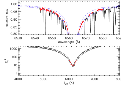
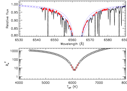
Figure 1: Fits to H$\alpha$ regions of WASP-94A (left) and -94B (right) continuum-normalized spectra to determine $T_{eff}$. The red portions of the spectrum are the “clean” regions used for the $\chi^{2}$ minimization, where weak atomic features do not influence the fit. The blue solid line is the best fit, and the blue dotted lines are $\pm$200 K models. The bottom panels of both plots demonstrate the $\chi^{2}$ minimization procedure.

We performed several additional tests to check whether the assumed Sun-relative parameters for WASP-94B were indeed reliable. For $T_{eff}$, we used the [Fe/H] values from Table 2 (this work, Solar Reference) in the Casagrande et al. (2010) effective temperature-color calibration for ($V-J$), ($V-K$), ($V-H$), and ($J-K$), with $V$ as given in NV14 with assumed errors of 0.05 mag, and $JHK_{s}$ as given on Simbad. The average resulting $T_{eff}$ values are 6216$\pm$91 K for WASP-94A and 6096$\pm$79 K for WASP-94B, which are consistent with the Sun-relative parameters albeit with larger errors. As another test of precise $T_{eff}$s, we matched via $\chi^{2}$ minimization the observed H$\alpha$ Balmer lines with model fits from the theoretical grid of H$\alpha$ lines from Barklem et al. (2002), in a process detailed in Ramírez et al. (2014b) that includes a non-standard 2D-normalization of the CCD region around the line. This analysis (see Fig. 1) resulted in best-fit $T_{eff}$s of 6201$\pm$25 K for WASP-94A and 6121$\pm$30 K for WASP-94B, after applying the necessary $+$46 K offset necessary to make the H$\alpha$ temperatures from the solar spectra match the nominal solar $T_{eff}$ of 5777 K (as derived in Ramírez et al. 2014b). The H$\alpha$ effective temperatures are even closer to the values obtained from the A-B analysis described above (see Table 2, This work, WASP-94B Reference), including the $\Delta~{}T_{eff}$ (80 K from H$\alpha$ versus 86 K from A-B analysis).

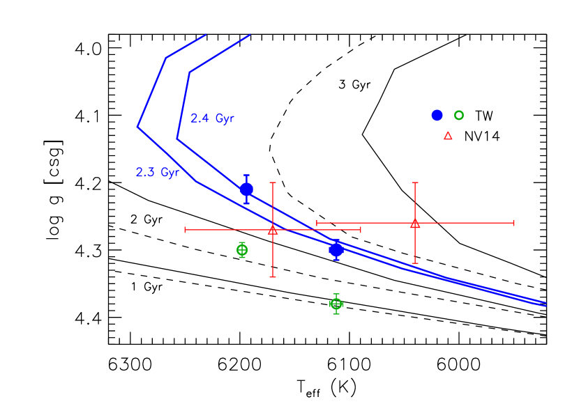
Figure 2: Evolutionary state test for precise surface gravities of WASP-94A and -94B. The solid/dashed lines are Yonsei-Yale/Padova isochrones of the noted ages. The red open triangles represent WASP-94A and -94B with the parameters of NV14. The green open circles show the parameters derived in the A-B parameter analysis, and listed in Table 2 under This work, WASP-94B Reference. The blue filled circles represent the same $T_{eff}$ values as the green points, but with log $g$ values shifted by $-$0.08 dex, providing better agreement for WASP-94A and -94B ages.

With confirmation of the $T_{eff}$ values derived in the A-B differential analysis, the derived log $g$ values can be checked against theoretical isochrones; if the stars are bound and coeval, their ages should be consistent. In Figure 2, the A-B parameters are plotted against Yonsei-Yale and Padova isochrones, and it is clear that the A-B log $g$ values result in different ages for the two stars (green open circles). However, if we assume that the surface gravities of both stars are 0.08 dex less (blue filled circles), then the stars both fall nicely on the 2.3 or 2.4 Gyr Yonsei-Yale isochrone (solid blue lines; both are consistent with 2.4 Gyr within errors). Thus, we fixed the log $g$ of WASP-94B to 4.30 dex, rather than 4.38 dex as originally determined relative to the Sun, and rederived the relative WASP-94A stellar parameters for each set of EW measurements. This resulted in very small changes in the other derived stellar parameters of WASP-94A (see Table 2, This work, WASP-94B Reference, Isochrone Log $g$). Given the lower log $g$ values are more consistent with the same age for both stars, these are used in the subsequent elemental abundance analysis. Lowering the log $g$ values by 0.08 (B)/0.09 (A) dex did not result in changes to the elemental abundance ratios (detailed in the next section) outside the original errors derived from the higher log $g$ values.

The isochrone analysis presented here indicates that the stars have an age of $\sim$2.5 Gyr (with an error of a few tenths of a Gyr), significantly younger than the age reported in NV14, $\sim$4 Gyr. The best matching age based on the Yonsei-Yale isochrones in Figure 2 (blue solid lines) is 2.3-2.4 Gyr, whereas the best matching age based on the Padova isochrones is more like 2.8 Gyr, still significantly younger than the 4 Gyr age reported in NV14.

3.2 Elemental Abundances

With knowledge of the environment in which spectral lines form, we can translate EW measurements of other elements into abundances via a curve-of-growth analysis within MOOG. The EWs of lines measured in the Sun, WASP-94A, and WASP-94B corresponding to 23 elements, including Fe, are listed in Table 1. Our procedure for measuring EWs in WASP-94A and -94B included a direct comparison in the normalized and Doppler-corrected spectra of every line. This allowed us to choose a continuum region that was the same in both spectra, reducing potential systematic error, and check for differences in the lines that may affect the upper and lower limits of the EW fit (e.g., if we want to avoid a blend). Carbon abundances were measured from both C I and CH lines, and for Sc, Ti, and Cr lines from both neutral and singly-ionized species were measured (in addition to Fe). Hyperfine structure corrections were employed for V, Mn, Co, Cu, Rb, Y, and Ba, and we applied the O triplet non-LTE corrections from Ramírez et al. (2007). The relative abundances obtained from a line-by-line analysis, averaged over three independent EW measurements, are listed in Table 3, along with errors that add in quadrature both the line-to-line scatter ($\sigma/\sqrt{n-1}$) as well as the errors propagated from each parameter uncertainty. For species with only one line (K I, Zr II), we adopted the largest line-to-line scatter for species with more than three lines available, within each set of independent EW measurements (the value of the largest line-to-line scatter was different for each of the measurement sets).

The NLTE corrections to the O I triplet line around 7775 Å are uncertain, and several different groups have published corrections. While our strictly differential approach between the two “twin” star should help eliminate uncertainty in the $\Delta$[O/H] values, we checked our results by performing a synthesis analysis of the [O I] line at 6300 Å using the MOOG synth driver, as outlined in Teske et al. (2014), §3.1.1. The synthesis fitting of WASP-94A yielded absolute oxygen abundances (log$N$(O)) of 9.01-9.03, while fitting of WASP-94B yielded log$N$(O) values of 8.98-9.02, confirming a small positive $\Delta$[O/H] for (A-B) that is represented by our reported error (0.006 dex). We also confirmed our negative $\Delta$[C/H] value by synthesis fitting two blended C₂ molecular features at 5086.3 Å and 5135.6 Å via the process outlined in Teske et al. (2013), §2.3.1. The fitted log$N$(C) of WASP-94A ranged from 8.63-8.65, and from 8.66-8.68 for WASP-94B, resulting in $\Delta$[C/H] (A-B) values between -0.05 and -0.02, within our reported errors for $\Delta$[C/H]. Importantly, we confirm that the $\Delta$[C/H] value is certainly below the zero line.

NV14 reported Li abundances log $N$(Li)${}_{A}=$2.10$\pm$0.07 and log $N$(Li)_B $\leq$1.20. They propose that the WASP-94 stars have already undergone magnetic breaking and Li depletion due to their low log$N$(Li) and $v$sin$i$ values. We confirm the low log$N$(Li) abundances in WASP-94AB, and a significant (A-B) difference, based on a synthesis analysis of the 6707.8 Å doublet using the line list of Mandell, Ge & Murray (2004). Our synthesis fitting suggests WASP-94A’s log$N$(Li)$=$2.01-2.04 and WASP-94B’s log$N$(Li)$\leq$1.62, resulting in a $\Delta$log$N$(Li)$\geq$0.39. Several authors have suggested that the formation of planets could enhance lithium depletion in host star photospheres (Gonzalez 2008, 2014; Israelian et al. 2009; Figueira et al. 2014; Delgado Mena et al. 2015) due to planetary migration (Castro et al. 2008), and/or star-disk interactions (e.g., Bouvier 2008), but there is not yet consensus due to selection biases in planet host samples and large lithium abundance uncertainties (e.g., Ghezzi et al. 2010; Baumann et al. 2010; Ramírez et al. 2012). Both WASP-94 stars border the “lithium desert” proposed by Ramírez et al. (2012), a region in $T_{eff}$ versus log$N$(Li) space devoid of stars. Indeed, there are no exoplanet host stars included in Ramírez et al. (2012) with as low log$N$(Li) and as high $T_{eff}$ and [Fe/H] as WASP-94B (see their Figure 9), making WASP-94B a slightly unusual case. The star’s relatively low log$N$(Li) suggests it may have experienced some short-lived surface destruction of lithium. Here we do not focus on the study of lithium, but the difference between WASP-94A and -94B, a pair of hot “twin” stars both hosting close-in giant planets, could prove to be a powerful tool for better understanding whether there is a connection between lithium depletion in stars and the presence of planets.

4 Discussion

4.1 Results: $\Delta$[X/H] vs. $T_{c}$

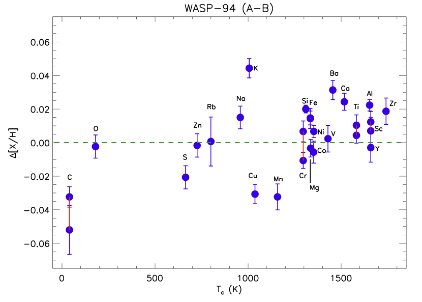
Figure 3: The $\Delta$(A-B) relative abundances versus T_c (Lodders 2003), calculated using the derived (A-B) stellar parameters with log $g$ of B fixed to 4.3 dex (see last row of Table 2). This plot shows the abundances before removing absorption lines with EW$>$100 mÅ; Figure 4 shows the abundances after removing these lines. The only significant difference between the abundances in the two plots is the $\Delta$[Na/H] value, which is lower in Figure 4.

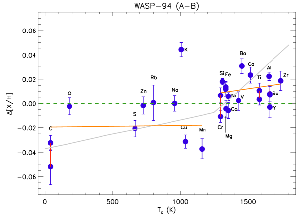
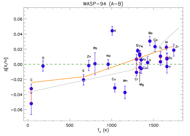
Figure 4: The $\Delta$(A-B) relative abundances versus T_c (Lodders 2003), calculated using the derived (A-B) stellar parameters with log $g$ of B fixed to 4.3 dex (see last row of Table 2). These plots show the abundances after removing absorption lines with EW$>$100 mÅ; O and K have only strong lines so are not removed. The only significant difference between the abundances in these plots and Figure 3 is the $\Delta$[Na/H] value, which is lower here. Also shown in orange are the best fits to the abundances, not including K, as discussed in §4.1.1, without (top) and with (bottom) a smooth $T_{c}$ break point. The grey lines shows the solar twin trend from Meléndez et al. (2009) with a constant 0.015 dex added to account for the [Fe/H] difference between A and B.

In Figure 3, the abundance differences between the two stars, $\Delta$[X/H], are plotted against the 50% condensation temperatures ($T_{c}$) from Lodders (2003) for solar composition gas. There is a small but significant (see below) enhancement of high-$T_{c}$ elements ($\geq$1200 K) in WASP-94A relative to -94B. Lodders (2003) refers to phosphorous at $T_{c}=1229$ K as “moderately volatile”, sulfur at $T_{c}=664$ K as “volatile”, and iron, magnesium, and silicon ($T_{c}=1334,1529,1397$ K, resp.) as “common”. As in other studies looking for correlations between abundance differences and condensation temperature, the $T_{c}$ values we use here are for a solar-composition gas. However, $T_{c}$ values will depend on the composition of the gas, which in the case of WASP-94AB is super-solar. Detailed chemical equilibrium condensation sequence calculations such as those in Bond et al. (2010) are beyond the scope of this work, but the sequences calculated in that work for gas of similar composition to WASP-94AB indicate $T_{c}$ values do not increase more than a few tens of K. Even in the high-metallicity condensation sequences where $T_{c}$ for C and O increase by up to about 1000 K, this would not affect our overall results because our “break” between volatiles and refractories is likely higher than $\sim$1000 K (see below). Most of the lower $T_{c}$ volatile or moderately volatile elements are depleted in WASP-94A, save sodium (Na) and potassium (K). The latter is based on one saturated line that suffers from a large NLTE effect ($\sim$0.3 dex; e.g., de La Reza and Müller 1975; Zhang et al. 2006); this abundance may thus not be very accurate. In an attempt to ameliorate the high $\Delta$[Na/H] value, as well as check for systematic error, the elemental abundance derivation was repeated across all elements, removing any potentially-saturated lines with EW values $>$100 mÅ. The resulting values are shown in Figure 4, with K and O unchanged, as their abundances are based on only strong lines. None of the new abundance derivations that exclude strong lines change within the errors, except for Na, which is exactly zero when two strong lines are removed from the average; removing these lines also reduces the line-to-line scatter, slightly decreasing the $\Delta$[Na/H] error.

4.1.1 Linear 1- and 2-Component Fits

Examining the new abundances in Figure 4 and excluding K, there appears to be a natural break point around $T_{c}=1200$ K, between Mn and Cr, although with moderate scatter ($\sigma$ of all $\Delta$[X/H]$=$0.02 dex). The $\chi^{2}$ value of a simple zero-slope, zero-intercept fit (the dashed green line in Figure 4) is 1.48. A weighted linear fit to the data with a forced-zero slope but a free intercept results in an intercept$=0.0055\pm 0.0010$ dex, and a $\chi^{2}$ value of 1.50, slightly worse than a flat line with intercept$=0$. A linear fit to the data with an unconstrained slope results in an intercept of -0.0302$\pm$0.0037 dex and a slope of 2.7723$\pm$0.2795$\times$10^-5 dex/K, with a $\chi^{2}$ value of 0.86 and a mean scatter around the fit of -0.0035 dex. The data thus support a non-zero slope at the $\sim$10$\sigma$ level.

To test whether a two-component linear function is favored (results in a lower $\chi^{2}$ value), we first repeat a linear fit to all the points (except $\Delta$[K/H]), removing the highest-$T_{c}$ point from each iteration to find the number of points whose linear fit results in the lowest slope value. The slope minimum occurs at $T_{c}=$1158 (Mn). This minimum is then used as $P[2]$ in a custom fit, executed with the IDL MPFITFUN routine (Markwardt 2009), with the functional form $[P[0]+P[1]\times X[0:P[2]],P[3]+P[4]\times X[P[2]+1,*]]$, where $P[0],P[1],P[3]$ and $P[4]$ are allowed to vary, $X$ corresponds to $T_{c}$, and $*$ is the last entry in $X$. The resulting best-fit parameters are $P[0]=$-0.0197$\pm$0.005 dex, $P[1]=$1.463$\pm$5.996$\times 10^{-6}$ dex/K, $P[3]=$-0.0120$\pm$0.0114dex and $P[4]=$1.615$\pm$0.795$\times 10^{-5}$ dex/K. This two component linear fit has a $\chi^{2}$ value of 0.71, with a volatile element ($T_{c}<1200$ K) slope consistent with zero and a refractory element ($T_{c}>1200$ K) slope inconsistent with zero at the 2$\sigma$ level. This two component fit is shown in green in the top panel of Figure 4. The mean scatter around this two-component fit is -0.0023 dex, and using $T_{c}$=1200 K as the divider, we find weighted averages (and weighted standard deviations) of $\Delta$[X/H]=-0.019$\pm$-0.006 for volatiles (i.e., a deficiency detected at the 3$\sigma$ level) and $\Delta$[X/H]=$+$0.011$\pm$0.002 for refractories (i.e., an enhancement detected at the 5$\sigma$ level).

As a second test of the $T_{c}$ break point, we performed two separate linear fits to the measurements, and varied the $T_{c}$-break temperature (where one fit ended and the other began) between 500 K and 1500 K. For each $T_{c}$-break temperature, we calculated the difference between the end of the low $T_{c}$ fit and the beginning of the high $T_{c}$ fit to find the value that resulted in a smooth transition between the two linear fits (zero difference between the end/start points). This $T_{c}$-break temperature is 685 K, much cooler than the 1200 K value found above. In this fit, the lower $T_{c}$ component has a slope 1.241$\pm$4.756$\times$10^-5 dex/K and an intercept of -0.0247$\pm$0.0167 dex, while the higher $T_{c}$ component slope of 3.829$\pm$1.233$\times$10^-5 dex/K and an intercept of -0.0424$\pm$0.0175 dex. Using $T_{c}$=685 K as the divider, we find weighted averages (and weighted standard deviations) of $\Delta$[X/H]=-0.022$\pm$-0.008 for volatiles (i.e., a deficiency detected at the 2$\sigma$ level) and $\Delta$[X/H]=$+$0.008$\pm$0.003 for refractories (i.e., an enhancement detected at the 2$\sigma$ level). However, the resulting fit shown in the bottom panel of Figure 4 has a $\chi^{2}$ of 0.936 and a mean scatter around the fit of -0.0053 dex, a slightly worse fit than the 2-component fit described above with a $T_{c}$-break point of 1200 K.

4.1.2 Nature of Scatter

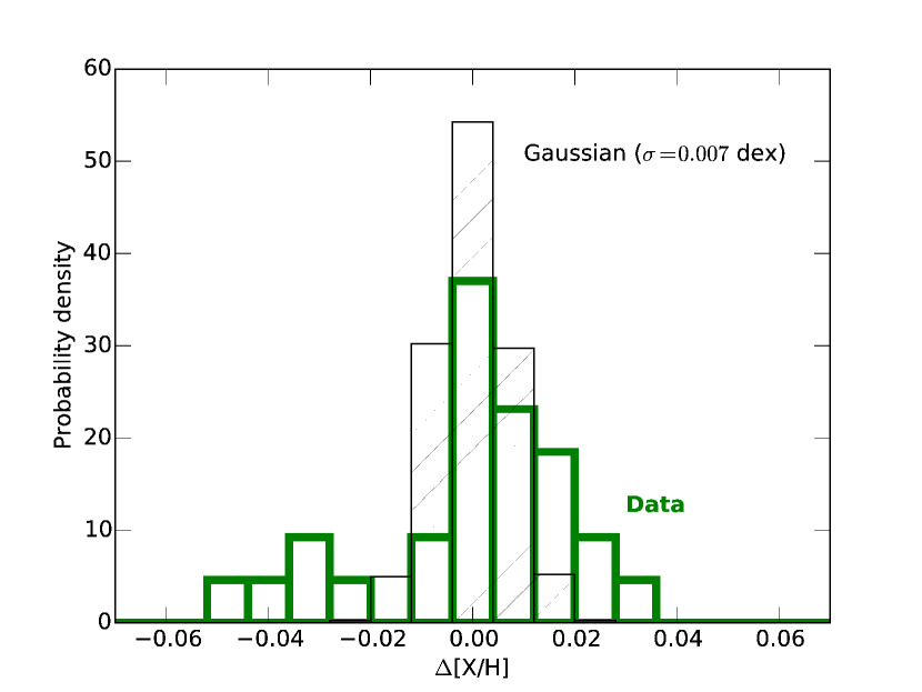
Figure 5: A histogram of normalized probability density of $\Delta$[X/H], comparing a sample “S” of 100,000 values randomly selected from a Gaussian distribution with $\sigma$=0.007 dex (black dashed bars) and our actual data (green open bars). It is clear that our data do not follow a normal distribution, and both a two-sample KS test and an AD test indicate the two samples are significantly different (see §4.1.2)

We ran standard statistical tests to address the question of whether the scatter seen in Figure 4 is consistent with random observational noise. These tests are independent of the $T_{c}$ correlation and only examine the level of scatter and its normality. For its use in some of these tests, we created a sample “S” of 100,000 $\Delta$[X/H] values randomly selected from a Gaussian distribution of $\sigma$=0.007 dex, which is the average error bar of our $\Delta$[X/H] values. A two-sample Kolmogorov-Smirnov (KS) test gives a $p$-value of 0.06 when comparing the actual data to the pure noise sample $S$. An Anderson-Darling (AD) test on the same two samples gives a significance level of 2.5$\times$10^-5. We repeated these tests assuming that our error bars had been underestimated and redefined the $S$ sample assuming Gaussian noise of $\sigma$=0.010 dex instead. In this case, we find a much larger KS $p$-value of $\sim$0.4, which would imply that our data could be compatible with no abundance difference within error, but the significance level from the AD test remains low, at 0.03. The AD test is known to be superior to the KS test for a variety of reasons, in particular its higher sensitivity to the edges of the distributions (see, e.g., Feigelson & Babu 2012, their Sect. 5.3.1). We also employed the AD and Shapiro-Wilk (SW) tests to quantify the “normality” of our $\Delta$[X/H] data set (these tests do not require an estimate of the sigma value a priori). In both cases, the statistic derived corresponds to a significance level below 6%. In other words, the probability that our $\Delta$[X/H] values correspond to a Gaussian distribution centered at zero is low. Despite having relatively few data points, the non-normality of our abudance differences can be clearly seen in Figure 5. Thus, these statistical tests suggest that there are in fact true abundance differences between the stars in the WASP-94 system.

As noted in §1.1, WASP-94 differs from the other known twin binary systems in which both stars host planets in several important ways. The trend with $\Delta$[X/H] and $T_{c}$ observed here – more refractory elements in WASP-94A than B, but fewer volatile elements – also differs from what is observed in the other known twin binary systems, including those in which only one star is known to host a planet. In every other published case, either no significant abundance differences are reported, or there is some degree of enhancement in all elements, including those with low $T_{c}$. The pattern observed here in WASP-94AB appears qualitatively similar to that reported by some authors in the 16 CygAB system (Ramírez et al. 2011; Tucci Maia et al. 2014) and reported in the XO-2AB system (Teske et al. 2015; Ramírez et al. 2015; Biazzo et al. 2015) – volatiles have a $\sim$flat slope, while refractories have a positive slope – but in WASP-94A the volatiles are depleted, not enhanced like in 16 Cyg A and XO-2N. Additionally, the differences we find here between WASP-94AB are smaller than those seen in 16 CygAB and XO-2AB, causing the appearance of our Figure 4 to be “noisier” due to the fact that it is “zoomed in” more than the previous cases (not because our errors are larger). Note, for example, that the enhancement of refractory element abundances compared to volatiles in solar twins relative to the Sun is about 2-3 times larger than that seen in WASP-94 A minus B, as shown by the thin gray line in Figure 4.

4.2 Explanation of Observed Trend

What could account for the observed trend in $\Delta$[X/H] abundances? Ramírez et al. (2015) explained the volatile depletion in XO-2S as potentially “more” gas giant planet formation around it versus XO-2N, leading to a relatively larger amount of volatile elements in -2N. Similarly, Tucci Maia et al. (2014) suggested the volatile depletion in 16 Cyg B relative to A as was due to the envelope of the giant planet around 16 Cyg B, and the refractory depletion was a signature of the rocky core of 16 Cyg Bb. Examining Figure 4, the volatile depletion in A could be explained by (more) giant planet formation causing a decrease in its overall metallicity, and thus volatile abundances, relative to B, and (more) rocky planet formation around B causing a decrease in its refractory abundances relative to A.

Alternatively, the observed abundance differences could be explained by the difference in metal content of WASP-94Ab and -94Bb, and not any additional planets. Miller & Fortney (2011) compared interior models of 14 cool transiting giant planets to their host stars’ [Fe/H] values, and found that the overall heavy element mass for planets ($M_{z}$) increases with planet mass, but that the percentage of metals in the planet versus the percentage of metals in the star ($Z_{pl}/Z_{star}$) decreases with planet mass, consistent with Solar System giant planets. If WASP-94Ab was larger, and thus had a smaller refractory-to-volatile abundance ratio than WASP-94Bb, then WASP-94A might contain less volatile but more refractory material “left behind” after the formation if its giant planet.

However, both of these explanations are unsupported by the planets actually observed. The planet around WASP-94B is more massive, so -94B should be the star to show the lower overall metallicity and volatile abundances, or the higher refractory-to-volatile ratio of “left over” material in the star. We can estimate whether the mass difference between WASP-94Ab and -94Bb can even explain the observed abundance differences using the corrected formula from Ramírez et al. (2011):

$$\Delta[M/H]=\mathrm{log}\bigg{[}\frac{(Z/X)_{cz}M_{cz}+(Z/X)_{P}M_{p}}{Z/X_{cz}(M_{cz}+M_{p})}\bigg{]}$$ (1)

with the convection zone mass $M_{cz}$ estimated as 0.0032 M_⊙ from the relation in Pinsonneault et al. (2001), $(Z/X)_{p}$ estimated as 0.1, $M_{p}$ as the mass difference between Ab and Bb (0.166 M_J, using Bb’s $Msini$), and $(Z/X)_{cz}$ estimated by scaling Asplund et al. (2009)’s $(Z/X)_{\odot}=0.134$ to WASP-94A’s [Fe/H] (0.32 dex). The required $\Delta$[M/H] for 0.166 M_J of material “added to” or “missing from” WASP-94A is $\sim$0.05 dex, much higher than the volatile/refractory abundance differences of 0.02/0.01 dex. A similar excercise for WASP-94B still results in $\sim$0.03 dex of material, which is more than is “missing” or “added” to WASP-94B. Furthermore, if as suggested as one source of the refractory enhancement in XO-2N (Teske et al. 2015; Ramírez et al. 2015; Biazzo et al. 2015), the refractory enhancement seen in this system is due to the migration of a giant planet pushing/dragging rocky material on to the star, why is this accretion signature seen in the star (A) with the least massive planet, which would presumably have a smaller gravitational effect on rocky material in the disk?

One can reverse the accretion equation, and instead solve for the mass of material that could explain the missing 0.02 dex of volatile/excess 0.01 dex of refractory material in WASP-94A (or the excess 0.02/missing 0.01 dex in -94B). In WASP-94A, which likely has a somewhat smaller convection zone than the cooler -94B, a deficit of 0.02 dex of $(Z/X)_{p}=0.1$ material requires $\sim$0.063 M_J of material to be “missing”. In WASP-94B, an enhancement of 0.02 dex of $(Z/X)_{p}=0.1$ material requires $\sim$0.098 M_J of material to be “added”. These masses are likely too small to be single bodies responsible for dynamical effects, e.g., a giant planet affecting the orbits and/or migration of either WASP-94Ab or -94Bb (Chatterjee et al. 2008; Ford & Rasio 2008). However, such masses could correspond to super-Earth or Neptune-sized planets (or amounts of material). This material could have been scattered inward (increasing the stellar abundance) or outward (decreasing the stellar abundance) by planet-planet interactions that may have caused the orbit misalignment and retrograde orbit of WASP-94Ab (e.g., Bromley & Kenyon 2011; Bromley & Kenyon 2014). Alternatively, these bodies could have been accreted onto the star during the inward migration of WASP-94Bb (Raymond et al. 2011; Fogg & Nelson 2005), which has near-zero $e$ (0.13$\pm$0.20, NV14). Figure 1 from Kaib et al. (2013) suggests that a binary like WASP-94 has a $\sim$0.5 instability fraction, and a rather large critical pericenter ($\sim$200 AU), meaning that if the binary separation evolved at all during the short lifetime of the stars, an instability would be more likely.

The above estimations assume a bulk $(Z/X)_{p}=0.1$ for planetary mass material, based on what is known about the giant planets in the Solar System (Guillot 2005; Fortney & Nettelmann 2010) and other giant exoplanets (Miller & Fortney 2011). However, if this value were smaller or larger, the effect on the stellar abundances would correspondingly decrease or increase. The value of $(Z/X)_{p}$ is not constant across Solar System planets, nor is it independent from the size of the envelope versus the core of the planet (e.g., Fortney & Nettelmann 2010). The proportion of volatile to refractories depends on the formation location, mass, and interior differentiation of planets; our model above is only a first-order estimation and future studies should more thoroughly test the impact of differentiated planet formation on stellar abundances.

The above calculations also assume a current $M_{cz}$ based on the mass of the star, but $M_{cz}$ is known to vary greatly across stellar lifetimes (Hayashi 1981; D’Antona & Mazzitelli 1994; Serenelli et al. 2011). Ramírez et al. (2011) explored how varying both $M_{cz}$ and $(Z/X)_{p}$ changed the amount of material required to account for the abundance difference between 16 Cyg A and B (see their Figure 12), based on both standard stellar models (Serenelli et al. 2011) and non-standard models of episodic accretion (Baraffe & Chabrier 2010). At earlier times when the stellar convection zone is a significant fraction ($\gtrsim$10%) of the mass of the star, a larger or more metal-rich amount of accreted material is required to cause the same stellar abundance change. For instance, a $M_{cz}=0.01M_{\odot}$ for WASP-94A would require $\sim$0.20 $M_{J}$ of material to cause a 0.02 dex difference, over 3$\times$ as much material than the smaller (current) $M_{cz}=0.0032M_{\odot}$ case. This might be one way to help explain a mass difference of $\geq$0.166 $M_{J}$, as observed between WASP-94Ab and -94Bb, but again the trend is opposite of what is expected (A is depleted by $\sim$0.20 $M_{J}$, not B), and it still leaves the refractory abundance enhancement in WASP-94A unresolved.

Perhaps what is most intriguing is why two “twin” similar stars formed apparently different planets. The planet around WASP-94A is less massive and misaligned with the stellar orbital axis, and likely retrograde, both signatures of dynamical interactions in the history of the planet’s formation and evolution. Why does WASP-94B appear to be circularized? The $T_{eff}$ of both stars put them near the $T_{eff}$ border that Winn et al. (2010) and Schlaufman (2010) suggest separates systems in which tidal dissipation damps planetary obliquities within a few Gyr and systems in which dissipation is ineffective (stars hotter than 6250 K). Winn et al. (2010) explain this break point as where the convection zone mass of stars becomes negligible. Based on the relation in Pinsonneault et al. (2001), WASP-94A’s $M_{cz}$ is between $\sim$0.003 and 0.004 M_⊙, while WASP-94B’s is between $\sim$0.005 and 0.006 M_⊙. Perhaps the 2$\times$ larger convection zone of WASP-94B versus -94A was enough to better facilitate tidal circularization of its giant planet.

Another possibility is that the abundance differences are due to or influenced by the orbital dynamics of the system. There may be a very stellar distant companion to WASP-94A or -94B, which would not have formed out of the protoplanetary disk and thus be undetectable in the abundance signatures, nor detectable in the limited RV coverage ($\sim$2 years). We are conducting high-contrast imaging observations to search for any such wide, massive perturbers, which may or may not be bound to either star, that could provide clues to the dynamical history of this system.

It may be that the small differences that have been observed in the high-precision abundances of planet-host stars are not related to planet formation. Önehag et al. (2011) suggest that the Sun’s peculiar abundance trend with $T_{c}$ is not due to small planet formation, but removal of refractory dust material early on in the Sun’s life. They applied a strictly differential (versus the Sun) approach to M67-1194, a solar twin in the M67 open cluster, to minimize systematic errors and determined not only that its parameters are indistinguishable from the Sun (except for [Fe/H]= 0.023$\pm$0.015 dex), but also that its abundance pattern very closely resembles the Sun, unlike the solar twins in Meléndez et al. (2009). The authors suggest that M67-1194 and the Sun may be from the same cluster, or at least that the Sun was born in a cluster similar to M67, and that both stars were affected during their fully-convective phase by dust cleansing by luminous stars in the same cluster. In Önehag, Gustafsson, & Korn (2014), the authors expand their sample to 14 M67 stars and find a similar agreement between the stars’ abundances and the Sun’s, which they use as further support for their hypothesis of dust cleansing in both protostellar clouds that formed the M67 stars and the Sun (which are perhaps the same). (We note, however, that Pichardo et al. (2012) present strong dynamical arguments that reject M67 as a parent cluster of the Sun.) Adibekyan et al. (2014) explored a large sample of solar-like stars and found possible correlations between the $\Delta$[X/H] vs. $T_{c}$ slopes and stellar ages, and between the slopes and mean galactocentric distance. The authors thus suggest that differences in $\Delta$[X/H] vs. $T_{c}$ slopes may not be related to planet formation at all, but instead to the age and galactic birth place of a given star (see, however, Spina et al. 2015). Gaidos (2015) pointed out that the trend of increasing $\Delta$[X/H] with $T_{c}$ seen in Meléndez et al. (2009) is the opposite of the pattern of element depletion in interstellar medium (ISM) gas (Yin 2005), and suggested that it may simply be a signature of gas-dust segregation and the particular composition of the dust in the protoplanetary disk. Unfortunately, none of the above explanations can naturally explain the differences reported here between WASP-94A and B if the assumption that they formed from the same gas cloud and are coeval holds.

Finally, the $\Delta$[X/H] values we measure may be due to the different rotation or granulation in WASP-94A versus -94B. NV14 measured $v$sin$i$ of 4.2 km s^-1 for WASP-94A and $<$1.5 km s^-1 for WASP-94B; while rotational broadening will not affect the total absorption (measured EW) of an individual line, rotational broadening can make blends harder to exclude. The iron line list used here, from Ramírez et al. (2014), was constructed specifically to exclude blended lines, but they are not always avoidable for other elements if there are only a few observable lines. In such cases (of which there are only a few; most elements measured have more than a few lines), we are careful to choose the same continuum and line boundaries in both stars such that the blended feature does not influence the EW fit. NV14 also used the cross-correlation function (CCF) bisector spans, measured as part of their radial velocity analysis, to confirm the planetary nature of WASP-94Ab and -94Bb, and found a $\sim$25 m s^-1 difference in the average CCF bisector values between the two stars (see their Figures 2 & 4). Line bisectors – the midpoints of the horizontal segments across the wings of a spectral line – are a diagnostic of granulation in stellar atmospheres. However, NV14 do not measure the bisector of spectral lines, but the CCF. Also, the 25 m s^-1 (A-B) difference is an order of magnitude smaller than the absolute bisector span measured in T${}_{eff}\sim$6000 K stars (e.g., Ramírez et al. 2008), which is already below the resolution of our spectra where the lines have been smoothed to be almost Gaussian. Thus, the CCF bisector span differences between WASP-94A and -94B are likely not meaningful to our differential abundance analysis.

5 Conclusions

Here we report differences in the abundances of two hot Jupiter hosting F-type stars that are in a wide ($\sim$2700 AU) separation binary. The stars are “twins”, with an (A-B) $\Delta$T${}_{eff}=$82$\pm$7 K, $\Delta$log $g=$-0.08$\pm$0.019 dex, $\Delta$[Fe/H]$=$0.014$\pm$0.006 dex, and $\Delta\xi=$0.12$\pm$0.014 km s^-1. The abundance analysis presented here is strictly differential, allowing a minimization of systematic errors, and includes the average across three independent equivalent width measurement sets, further reducing observational errors. One tangible result of this work is the reduction in age of the host stars by at least 1 Gyr. As a result of our careful stellar parameter determination, we could pinpoint the isochrone on which both WASP-94A and -94B fell, based on their respective $T_{eff}$s and log $g$s. This results in an age between 2.3 and 2.8 Gyr (not including measurement error of a few tenths of a Gyr), depending on the isochrone used, which is significantly younger than the $\sim$4 Gyr age reported in NV14.

We find evidence of a non-zero slope trend between $\Delta$[X/H] vs. $T_{c}$ at the 10$\sigma$ level, with volatile element depletion (by $\sim$-0.02 dex, on average) and refractory element enhancement (by $\sim$0.01 dex, on average) in WASP-94A. This differs from all other stellar abundance studies of binary systems in which one or both stars host planets, and does not seem to match any previous explanations of such trends, due to the mass and orbital period differences between WASP-94Ab and -94Bb. While there is not an obvious explanation for these abundance differences right now, the precision achieved here, at the $\sim$0.005 dex level, allows us to examine differences that may have been effectively washed out in previous studies of binary stars, which suggested that anywhere from $\lesssim$0.015 dex to $\lesssim$0.03 dex differences were to be expected.

Whatever the cause, the abundance differences detected here for WASP-94AB, along with those seen in 16 CygAB and XO-2AB, challenge the long-standing assumption that stars in binary systems must share the same chemical composition at all times. The stars may have formed from a single composition cloud, but processes that occurred after their birth have certainly altered their surface compositions at the few percent level. A larger sample of “twin” systems with constraints on planet presence is necessary to better understand how curious the WASP-94AB system is or not.

Table 1: Measured Lines & Equivalent Widths

Ion	$\lambda$	$\chi$	log $gf$	EW⊙	WASP-94A	WASP-94A	WASP-94A	WASP-94B	WASP-94B	WASP-94B
	(Å)	(eV)	(dex)	(mÅ)	EWIR (mÅ)	EWSK (mÅ)	EWJT (mÅ)	EWIR (mÅ)	EWSK (mÅ)	EWJT (mÅ)
Fe I	4389.245	0.052	-4.583	73.2	74.2	73.4	74.1	75.6	74.8	75.9
Fe I	4445.471	0.087	-5.441	40.4	35.8	38.2	36.4	38.6	40.4	39.7
Fe I	4602.001	1.608	-3.154	72.3	78.7	79.0	79.4	78.8	79.6	80.2
Fe I	4690.14	3.69	-1.61	59.5	66.9	65.7	66.8	66.7	66.1	67.6
Fe I	4788.76	3.24	-1.73	67.7	74.8	74.4	73.1	74.3	74.5	72.6
Fe I	4799.41	3.64	-2.13	36.0	37.7	42.1	41.0	40.0	42.3	41.4
Fe I	4808.15	3.25	-2.69	27.6	28.9	28.6	29.3	31.0	31.3	30.9
Fe I	4950.1	3.42	-1.56	74.6	80.5	80.8	89.3	81.0	81.3	88.6
Fe I	4994.129	0.915	-3.08	102.0	108.2	108.9	108.6	107.2	109.0	108.5
Fe I	5141.74	2.42	-2.23	90.6	93.0	92.9	93.6	92.8	93.3	95.5
Fe I	5198.71	2.22	-2.14	99.2	103.0	103.8	104.5	103.5	104.3	104.7
Fe I	5225.525	0.11	-4.789	74.9	71.1	71.9	73.7	71.7	74.7	76.3
Fe I	5242.49	3.63	-0.99	87.7	95.9	96.8	96.9	95.1	96.7	96.1
Fe I	5247.05	0.087	-4.961	67.7	65.7	65.0	69.8	69.1	69.3	70.3
Fe I	5250.208	0.121	-4.938	66.8	62.7	61.1	73.0	66.1	65.7	73.6
Fe I	5295.31	4.42	-1.59	30.3	37.2	37.5	36.8	38.4	39.3	39.2
Fe I	5322.04	2.28	-2.89	62.3	66.9	68.2	66.5	68.7	69.4	68.5
Fe I	5373.71	4.47	-0.74	63.6	73.2	73.5	72.0	71.7	73.9	72.5
Fe I	5379.57	3.69	-1.51	62.4	69.5	69.5	69.9	70.9	71.2	70.2
Fe I	5386.33	4.15	-1.67	33.0	37.0	38.1	37.5	39.8	40.6	39.3
Fe I	5441.34	4.31	-1.63	32.3	37.9	38.8	37.9	39.9	40.5	39.3
Fe I	5466.396	4.371	-0.565	78.8	86.4	89.9	87.0	87.6	88.7	86.5

Note. — This table is available in its entirety in a machine-readable form online. A portion is shown here for guidance regarding its form and content.

Table 2: Stellar Parameters

Star	Teff	log $g$	$\rm{[Fe/H]}$	$\xi$
	(K)	[cgs]	(dex)	(km s-1)
NV14
WASP-94A	6170$\pm$80	4.27$\pm$0.07	0.26$\pm$0.15	$\cdots$
WASP-94B	6040$\pm$90	4.26$\pm$0.06	0.23$\pm$0.14	$\cdots$
$\Delta$(A-B)	$+$130$\pm$120	$+$0.01$\pm$0.09	$+$0.03$\pm$0.21	$\cdots$
This work, Solar Reference
WASP-94A	6198$\pm$8	4.30$\pm$0.021	0.318$\pm$0.006	1.44$\pm$0.016
WASP-94B	6112$\pm$6	4.38$\pm$0.015	0.305 $\pm$0.005	1.32$\pm$0.012
$\Delta$(A-B)	$+$86$\pm$10	$-$0.08$\pm$0.029	$+$0.013$\pm$0.008	$+$0.012$\pm$0.020
This Work, WASP-94B Reference
WASP-94A	6198$\pm$4	4.30$\pm$0.011	0.319$\pm$0.003	1.44$\pm$0.008
WASP-94B (same as solar ref.)	6112$\pm$6	4.38$\pm$0.015	0.305 $\pm$0.005	1.32$\pm$0.012
$\Delta$(A-B)	$+$86 $\pm$7	$-$0.08$\pm$0.019	$+$0.014$\pm$0.006	$+$0.12$\pm$0.014
This work, WASP-94B Reference, Isochrone Log $g$
WASP-94A	6194$\pm$5	4.21$\pm$0.011	0.320$\pm$0.004	1.43$\pm$0.008
WASP-94B (log $g$=4.3)	6112$\pm$6	4.30$\pm$0.015	0.305 $\pm$0.005	1.32$\pm$0.012
$\Delta$(A-B)	$+$82 $\pm$7	$-$0.09$\pm$0.019	$+$0.015$\pm$0.006	$+$0.11$\pm$0.014

Table 3: Derived $\Delta$(A-B) Abundances

Species	Tc	A-B Params, log $g_{\rm{B}}=4.3$		A-B Params, log $g_{\rm{B}}=4.3$, no strong lines
		$\Delta$[X/H]	error	$\Delta$[X/H]	error
	(K)	(dex)	(dex)	(dex)	(dex)
C I	40	-0.032	0.006	-0.032	0.006
CH	40	-0.052	0.015	-0.052	0.015
O I	180	-0.002	0.007	-0.0021	0.007
Na I	958	0.015	0.007	0.000	0.006
Mg I	1336	-0.003	0.005	-0.004	0.007
Al I	1653	0.022	0.003	0.022	0.003
Si I	1310	0.020	0.002	0.018	0.003
S I	664	-0.021	0.007	-0.021	0.007
K I	1006	0.044	0.006	0.0441	0.006
Ca I	1517	0.024	0.005	0.023	0.007
Sc I	1659	0.007	0.008	0.007	0.008
Sc II	1659	0.012	0.006	0.008	0.006
Ti I	1582	0.004	0.005	0.003	0.005
Ti II	1582	0.010	0.006	0.011	0.006
V I	1429	0.002	0.008	0.002	0.008
Cr I	1296	-0.011	0.005	-0.011	0.005
Cr II	1296	0.007	0.006	0.007	0.006
Mn I	1158	-0.032	0.008	-0.037	0.008
Fe I	1334	0.015	0.004	0.014	0.004
Fe II	1334	0.014	0.006	0.012	0.006
Co I	1352	-0.006	0.007	-0.006	0.007
Ni I	1353	0.007	0.004	0.006	0.003
Cu I	1037	-0.031	0.006	-0.031	0.005
Zn I	726	-0.002	0.007	-0.002	0.007
Rb I	800	0.001	0.015	0.001	0.015
Y II	1659	-0.003	0.008	-0.003	0.009
Zr II	1741	0.019	0.008	0.019	0.008
Ba II	1455	0.031	0.006	0.031	0.006

References

- Adibekyan et al. (2012) Adibekyan, V. Z., Santos, N. C., Sousa, S. G., et al. 2012, A&A, 543, A89
- Adibekyan et al. (2014) Adibekyan, V. Z., González Hernández, J. I., Delgado Mena, E., et al. 2014, A&A, 564, L15
- Asplund et al. (2009) Asplund, M., Grevesse, N., Sauval, A. J., & Scott, P. 2009, ARA&A, 47, 481
- Baraffe & Chabrier (2010) Baraffe, I., & Chabrier, G. 2010, A&A, 521, A44
- Barklem et al. (2002) Barklem, P. S., Stempels, H. C., Allende Prieto, C., et al. 2002, A&A, 385, 951
- Baumann et al. (2010) Baumann, P., Ramírez, I., Meléndez, J., Asplund, M., & Lind, K. 2010, A&A, 519, A87
- Bensby et al. (2014) Bensby, T., Feltzing, S., & Oey, M. S. 2014, A&A, 562, A71
- Bernstein et al. (2003) Bernstein, R., Shectman, S. A., Gunnels, S. M., Mochnacki, S., & Athey, A. E. 2003, Proc. SPIE, 4841, 1694
- Biazzo et al. (2015) Biazzo, K., Gratton, R., Desidera, S., et al. 2015, arXiv:1506.01614
- Bond et al. (2010) Bond, J. C., O’Brien, D. P., & Lauretta, D. S. 2010, ApJ, 715, 1050
- Bouvier (2008) Bouvier, J. 2008, A&A, 489, L53
- Bromley & Kenyon (2011) Bromley, B. C., & Kenyon, S. J. 2011, ApJ, 735, 29
- Bromley & Kenyon (2014) Bromley, B. C., & Kenyon, S. J. 2014, ApJ, 796, 141
- Buchhave & Latham (2015) Buchhave, L. A., & Latham, D. W. 2015, ApJ, 808, 187
- Burke et al. (2007) Burke, C. J., McCullough, P. R., Valenti, J. A., et al. 2007, ApJ, 671, 2115
- Casagrande et al. (2010) Casagrande, L., Ramírez, I., Meléndez, J., Bessell, M., & Asplund, M. 2010, A&A, 512, A54 Castro et al. 2008
- Chatterjee et al. (2008) Chatterjee, S., Ford, E. B., Matsumura, S., & Rasio, F. A. 2008, ApJ, 686, 580
- Chambers (2010) Chambers, J. E. 2010, ApJ, 724, 92
- D’Antona & Mazzitelli (1994) D’Antona, F., & Mazzitelli, I. 1994, ApJS, 90, 467
- da Silva et al. (2015) da Silva, R., Milone, A. d. C., & Rocha-Pinto, H. J. 2015, A&A, 580, A24
- Damasso et al. (2015) Damasso, M., Biazzo, K., Bonomo, A. S., et al. 2015, A&A, 575, A111
- de La Reza & Mueller (1975) de La Reza, R., & Mueller, E. A. 1975, Sol. Phys., 43, 15
- Deacon et al. (2015) Deacon, N. R., Kraus, A. L., Mann, A. W., et al. 2015, arXiv:1509.04712
- Desidera et al. (2004) Desidera, S., Gratton, R. G., Scuderi, S., et al. 2004, A&A, 420, 683
- Desidera et al. (2006) Desidera, S., Gratton, R. G., Lucatello, S., & Claudi, R. U. 2006, A&A, 454, 581 Epstein et al. 2010
- Everett et al. (2013) Everett, M. E., Howell, S. B., Silva, D. R., & Szkody, P. 2013, ApJ, 771, 107 Feigelson & Babu 2012
- Fischer & Valenti (2005) Fischer, D. A., & Valenti, J. 2005, ApJ, 622, 1102
- Fogg & Nelson (2005) Fogg, M. J., & Nelson, R. P. 2005, A&A, 441, 791
- Ford & Rasio (2008) Ford, E. B., & Rasio, F. A. 2008, ApJ, 686, 621
- Fortney & Nettelmann (2010) Fortney, J. J., & Nettelmann, N. 2010, Space Sci. Rev., 152, 423
- Gaidos (2015) Gaidos, E. 2015, ApJ, 804, 40
- Ghezzi et al. (2010) Ghezzi, L., Cunha, K., Smith, V. V., et al. 2010, ApJ, 720, 1290
- Goldreich & Tremaine (1980) Goldreich, P., & Tremaine, S. 1980, ApJ, 241, 425
- González Hernández et al. (2010) González Hernández, J. I., Israelian, G., Santos, N. C., Sousa, S., Delgado-Mena, E., Neves, V., Udry, S., 2010, ApJ, 720, 1592
- González Hernández et al. (2013) González Hernández, J. I., Delgado-Mena, E., Sousa, S. G., et al. 2013, A&A, 552, A6
- Gonzalez (2008) Gonzalez, G. 2008, MNRAS, 386, 928
- Gonzalez (2014) Gonzalez, G. 2014, MNRAS, 441, 1201
- Gratton et al. (2001) Gratton, R. G., Bonanno, G., Claudi, R. U., et al. 2001, A&A, 377, 123
- Guillochon et al. (2011) Guillochon, J., Ramirez-Ruiz, E., & Lin, D. 2011, ApJ, 732, 74
- Guillot (2005) Guillot, T. 2005, Annual Review of Earth and Planetary Sciences, 33, 493
- Gustafsson et al. (2008) Gustafsson, B., Edvardsson, B., Eriksson, K., et al. 2008, A&A, 486, 951
- Hayashi (1981) Hayashi, C. 1981, Progress of Theoretical Physics Supplement, 70, 35
- Hellier et al. (2011) Hellier, C., Anderson, D. R., Collier Cameron, A., et al. 2011, European Physical Journal Web of Conferences, 11, 01004
- Jones et al. (2006) Jones, H. R. A., Butler, R. P., Tinney, C. G., et al. 2006, MNRAS, 369, 249
- Kaib et al. (2013) Kaib, N. A., Raymond, S. N., & Duncan, M. 2013, Nature, 493, 381
- Lissauer et al. (2014) Lissauer, J. J., Marcy, G. W., Bryson, S. T., et al. 2014, ApJ, 784, 44
- Liu et al. (2014) Liu, F., Asplund, M., Ramírez, I., Yong, D., & Meléndez, J. 2014, MNRAS, 442, L51
- Lodders (2003) Lodders, K. 2003, ApJ, 591, 1220
- Mack et al. (2014) Mack, C. E., III, Schuler, S. C., Stassun, K. G., & Norris, J. 2014, ApJ, 787, 98
- Mandell et al. (2004) Mandell, A. M., Ge, J., & Murray, N. 2004, AJ, 127, 1147
- Markwardt (2009) Markwardt, C. B. 2009, Astronomical Data Analysis Software and Systems XVIII, 411, 251
- Mayor et al. (2011) Mayor, M., Marmier, M., Lovis, C., et al. 2011, arXiv:1109.2497
- Meléndez et al. (2009) Meléndez, J., Asplund, M., Gustafsson, B., & Yong, D. 2009, ApJ, 704, L66
- Miller & Fortney (2011) Miller, N., & Fortney, J. J. 2011, ApJ, 736, L29
- Naoz et al. (2011) Naoz, S., Farr, W. M., Lithwick, Y., Rasio, F. A., & Teyssandier, J. 2011, Nature, 473, 187
- Neveu-VanMalle et al. (2014) Neveu-VanMalle, M., Queloz, D., Anderson, D. R., et al. 2014, A&A, 572, A49
- Nissen (2015) Nissen, P. E. 2015, A&A, 579, A52
- Önehag et al. (2011) Önehag, A., Korn, A., Gustafsson, B., Stempels, E., & Vandenberg, D. A. 2011, A&A, 528, A85
- Önehag et al. (2014) Önehag, A., Gustafsson, B., & Korn, A. 2014, A&A, 562, A102
- Pichardo et al. (2012) Pichardo, B., Moreno, E., Allen, C., et al. 2012, AJ, 143, 73
- Pinsonneault et al. (2001) Pinsonneault, M. H., DePoy, D. L., & Coffee, M. 2001, ApJ, 556, L59
- Ramírez et al. (2008) Ramírez, I., Allende Prieto, C., & Lambert, D. L. 2008, A&A, 492, 841
- Ramírez et al. (2009) Ramírez, I., Meléndez, J., & Asplund, M. 2009, A&A, 508, L17
- Ramírez et al. (2010) Ramírez, I., Asplund, M., Baumann, P., Meléndez, J., & Bensby, T. 2010, A&A, 521, A33
- Ramírez et al. (2011) Ramírez, I., Meléndez, J., Cornejo, D., Roederer, I. U., & Fish, J. R. 2011, ApJ, 740, 76
- Ramírez et al. (2014) Ramírez, I., Meléndez, J., & Asplund, M. 2014, A&A, 561, A7
- Ramírez et al. (2015) Ramírez, I., Khanal, S., Aleo, P., et al. 2015, ApJ, 808, 13
- Rasio & Ford (1996) Rasio, F. A., & Ford, E. B. 1996, Science, 274, 954
- Raymond et al. (2011) Raymond, S. N., Armitage, P. J., Moro-Martín, A., et al. 2011, A&A, 530, A62
- Saffe et al. (2015) Saffe, C., Flores, M., & Buccino, A. 2015, A&A, 582, A17
- Santos et al. (2004) Santos, N. C., Israelian, G., & Mayor, M. 2004, A&A, 415, 1153
- Schuler et al. (2011) Schuler, S. C., Flateau, D., Cunha, K., King, J. R., Ghezzi, L., Smith, V. V., 2011b, ApJ, 732, 55
- Schuler et al. (2011) Schuler, S. C., Cunha, K., Smith, V. V., Ghezzi, L., King, J. R., Deliyannis, C. P., Boesgaard, A. M., 2011a, ApJ, 737, L32
- Serenelli et al. (2011) Serenelli, A. M., Haxton, W. C., & Peña-Garay, C. 2011, ApJ, 743, 24
- Schlaufman (2010) Schlaufman, K. C. 2010, ApJ, 719, 602
- Sneden (1973) Sneden, C. 1973, ApJ, 184, 839
- Sousa et al. (2008) Sousa, S. G., Santos, N. C., Mayor, M., et al. 2008, A&A, 487, 373
- Spina et al. (2015) Spina, L., Meléndez, J., & Ramírez, I. 2015, arXiv:1511.01012
- Teske et al. (2013) Teske, J. K., Schuler, S. C., Cunha, K., Smith, V. V., & Griffith, C. A. 2013, ApJ, 768, L12
- Teske et al. (2014) Teske, J. K., Cunha, K., Smith, V. V., Schuler, S. C., & Griffith, C. A. 2014, ApJ, 788, 39
- Teske et al. (2015) Teske, J. K., Ghezzi, L., Cunha, K., et al. 2015, ApJ, 801, L10
- Tucci Maia et al. (2014) Tucci Maia, M., Meléndez, J., & Ramírez, I. 2014, ApJ, 790, L25
- Winn et al. (2010) Winn, J. N., Fabrycky, D., Albrecht, S., & Johnson, J. A. 2010, ApJ, 718, L145
- Wright et al. (2012) Wright, J. T., Marcy, G. W., Howard, A. W., et al. 2012, ApJ, 753, 160
- Wu & Murray (2003) Wu, Y., & Murray, N. 2003, ApJ, 589, 605
- Wu & Lithwick (2011) Wu, Y., & Lithwick, Y. 2011, ApJ, 735, 109
- Yin (2005) Yin, Q. 2005, Chondrites and the Protoplanetary Disk, 341, 632
- Zhang et al. (2006) Zhang, H. W., Gehren, T., Butler, K., Shi, J. R., & Zhao, G. 2006, A&A, 457, 645