Nucleon Charges, Form-factors and Neutron EDM

Abstract:

We present an update of our analysis of statistical and systematic errors in the calculation of iso-vector scalar, axial and tensor charges of the nucleon. The calculations are done using $N_{f}=2+1+1$ flavor HISQ ensembles generated by the MILC Collaboration at three values of the lattice spacing ($a=0.12,\ 0.09,$ and $0.06$ fm) and three values of the quark mass ($M_{\pi}\approx 310,\ 220$ and $130$ MeV); and clover fermions for calculating the correlation functions, i.e., we use a clover-on-HISQ lattice formulation. The all-mode-averaging method allows us to increase the statistics by a factor of eight for the same computational cost leading to a better understanding of and control over excited state contamination. Our current results, after extrapolation to the continuum limit and physical pion mass are $g_{A}^{u-d}=1.21(3)$, $g_{T}^{u-d}=1.005(59)$ and $g_{S}^{u-d}=0.95(12)$. Further checks of control over all systematic errors, especially in $g_{A}^{u-d}$, are still being performed. Using results for the flavor-diagonal charges, $g_{T}^{u}$, $g_{T}^{d}$ and $g_{T}^{s}$, we analyze contributions of the quark electric dipole moment to the neutron EDM and the consequences for split SUSY model.

1 Introduction

The all-mode-averaging method allows us to obtain high precision estimates for the matrix elements of flavor-diagonal and isovector bilinear quark operators within nucleon states. These are needed to probe many exciting areas of the Standard Model (SM) and its extensions. In Ref. [1], we showed that new scalar and tensor interactions at the TeV scale could give rise to corrections at the $10^{-3}$ level in precision measurements of the helicity flip parts of the decay distribution of (ultra)cold neutrons (UCN). In Ref. [2], we described the calculation of flavor-diagonal tensor charges $g_{T}^{u}$, $g_{T}^{d}$ and $g_{T}^{u+d}$ and analyze constrains on BSM theories using the quark EDMs and the current bound on the neutron EDM [3].

In these proceedings, we first describe the level of control achieved over systematic errors, in particular the excited state contamination (ESC), using $O(50,000)$ measurements with the all-mode-averaging (AMA) method [5]. We then summarize our results for the iso-vector charges, the calculation of the flavor-diagonal tensor charges $g_{T}^{u}$, $g_{T}^{d}$ and $g_{T}^{u+d}$ and an analysis the contribution of quark EDM to the neutron EDM. These calculations were done using 9 ensembles of 2+1+1 flavor HISQ lattices generated by the MILC collaboration [4]. The matrix elements are calculated using clover valence quarks on these HISQ ensembles. A summary of the parameters of the nine HISQ ensembles analyzed and the number of measurements made in the fully high precision (HP) and the AMA calculations is given in Table 1.

2 All-mode-averaging Method

The all-mode-averaging (AMA) technique [5] allowed us to significantly increase the statistics very economically. The basic idea of the method is that one can construct correlation functions using quark propagators (inverse of the Dirac matrix) calculated with a low precision (LP) inversion criteria. The resulting bias can then be removed by calculating the difference between correlated HP and LP estimates using much fewer source positions. The unbiased estimate for the two ($C_{\text{LP}}^{\text{2pt}}$) and three ($C_{\text{HP}}^{\text{2pt}}$) point functions are given by

$$C^{\text{imp}}=\frac{1}{N_{\text{LP}}}\sum_{i=1}^{N_{\text{LP}}}C_{\text{LP}}(\mathbf{x}_{i}^{\text{LP}})+\frac{1}{N_{\text{HP}}}\sum_{i=1}^{N_{\text{HP}}}\left[C_{\text{HP}}(\mathbf{x}_{i}^{\text{HP}})-C_{\text{LP}}(\mathbf{x}_{i}^{\text{HP}})\right]\,,$$ (1)

with $N_{\rm HP}\ll N_{\rm LP}$. Here $\mathbf{x}_{i}^{\text{LP}}$ and $\mathbf{x}_{i}^{\text{HP}}$ are the two kinds of source positions on each configuration from which the LP and the HP correlators are calculated. Our AMA analysis done on five ensembles is described in detail in [2]. We use $64+4$ LP and 4 HP measurements on each configuration. These 4 HP source calculations are the same as used in the full high precision (HP) study presented in [2] and, therefore, needed no additional calculations. In total, the new simulations generated $4\times 16+4=68$ LP two- and three-point correlation functions per configuration. The statistics used in the HP and the AMA analyses are given in Table 1.

Label	$L^{3}\times T$	$M_{\pi}$ MeV	$(M_{\pi}L)$	$N_{\text{cfgs}}$	$N_{\text{HP}}$	$N_{\text{AMA}}$	$t_{\text{sep}}$
a12m310	$24^{3}\times 64$	305.3(4)	$4.54$	1013	8104	64832	8, 9, 10, 11, 12
a12m220S	$24^{3}\times 64$	218.1(4)	$3.22$	1000	12000		8, 10 12
a12m220	$32^{3}\times 64$	216.9(2)	$4.3$	958	7664		8, 10, 12
a12m220L	$40^{3}\times 64$	217.0(2)	$5.36$	1010	8080	68680	8, 10, 12, 14
a09m310	$32^{3}\times 96$	312.7(6)	$4.5$	881	7058		10, 12, 14
a09m220	$48^{3}\times 96$	220.3(2)	$4.71$	890	7120		10, 12, 14
a09m130	$64^{3}\times 96$	128.2(1)	$3.66$	883	4824	56512	10, 12, 14
a06m310	$48^{3}\times 144$	319.3(5)	$4.51$	865	3460	64000	16, 20, 22, 24
a06m220	$64^{3}\times 144$	229.2(4)	$4.25$	650	1320	41600	16, 20, 22, 24

Table 1: Description of the nine ensembles at $a=0.12$, $0.09$, $0.06$ fm used in this study. $N_{\text{HP}}$ denotes the number of measurements with high precision solves and $N_{\text{AMA}}$ with the AMA method.

3 Excited-State Contamination

The goal is to extract all observables (charges, charge radii, form factors, generalized parton distribution functions, TMDs) by calculating matrix elements between ground-state nucleons. Excited state contamination is, however, a significant challenge to the calculations of matrix elements within nucleon states [2]. We employ three strategies to control the ESC. (i) The overlap between the nucleon operator and the excited states is reduced by using smeared sources when calculating the quark propagators. (ii) We calculate the three-point correlation functions for a number of values of the source-sink separation $t_{\rm sep}$ given in Table 1. (iii) Data at various $t_{\rm sep}$ are fit simultaneously using the two-state ansatz given to estimate the $t_{\rm sep}\to\infty$ value as follows:

$$C^{\text{2pt}}(t_{f},t_{i})= {|{\cal A}_{0}|}^{2}e^{-M_{0}(t_{f}-t_{i})}+{|{\cal A}_{1}|}^{2}e^{-M_{1}(t_{f}-t_{i})}\,,$$

$$C^{\text{3pt}}_{\Gamma}(t_{f},\tau,t_{i})= |{\cal A}_{0}|^{2}\langle 0|\mathcal{O}_{\Gamma}|0\rangle e^{-M_{0}(t_{f}-t_{i})}+|{\cal A}_{1}|^{2}\langle 1|\mathcal{O}_{\Gamma}|1\rangle e^{-M_{1}(t_{f}-t_{i})}$$

$$+ \ \ {\cal A}_{0}{\cal A}_{1}^{*}\langle 0|\mathcal{O}_{\Gamma}|1\rangle e^{-M_{0}(\tau-t_{i})}e^{-M_{1}(t_{f}-\tau)}+{\cal A}_{0}^{*}{\cal A}_{1}\langle 1|\mathcal{O}_{\Gamma}|0\rangle e^{-M_{1}(\tau-t_{i})}e^{-M_{0}(t_{f}-\tau)}.$$ (2)

The masses and amplitudes $M_{0}$, $M_{1}$, ${\cal A}_{0}$, and ${\cal A}_{1}$ of the ground and “first” excited states are obtained from fits to the two-point functions. These are then used as inputs in the fit to the 3-point function to extract the three matrix elements $\langle 0|O_{\Gamma}|0\rangle$, $\langle 0|O_{\Gamma}|1\rangle$ and $\langle 1|O_{\Gamma}|1\rangle$. Propagation of errors between the two fits is taken into account by doing both within the same jackknife process.

Fig. 1 illustrates the improvement in the $a12m310$ ensemble data for the isovector charges on using the AMA method compared to all HP. The two estimates are consistent, with the errors in the AMA data smaller by $\approx\sqrt{8}$, consistent with the increase in the statistics: small enough to resolve the trend with $t_{\rm sep}$. We find that the two state fit captures these trends, significantly increasing the confidence in the fit to estimate the $t_{\rm sep}\to\infty$ value.

Fits to 2- and 3-point functions using Eq. (2) yield five physical quantities: the masses $M_{0}$ and $M_{1}$ and the three matrix elements: the charge $\langle 0|O_{\Gamma}|0\rangle$ and the ME $\langle 0|O_{\Gamma}|1\rangle$ and $\langle 1|O_{\Gamma}|1\rangle$, albeit ESC and discretization errors have to be removed from each. On the other hand, the two amplitudes, ${\cal A}_{0}$ and ${\cal A}_{1}$, depend on the nucleon interpolating operator and the smearing used at the source and sink ends of the quark propagator. From Eq. (2), it is clear that to reduce ESC one needs to reduce the ratio ${\cal A}_{1}/{\cal A}_{0}$. Our tests show that increasing the size of the Gaussian smearing reduces ESC in the charges, but beyond a certain size the errors in the correlation functions start to increase. A good compromise choice for the smearing parameter is $\sigma\approx 0.60$ fm, with $\sigma$ defined as in [2].

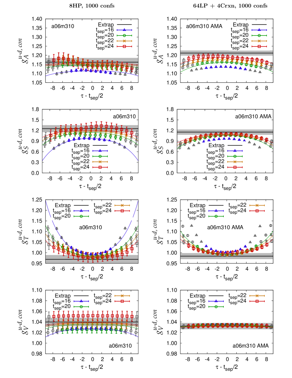
Figure 1: Figure illustrates reduction in errors between 8000 HP and 64,000 AMA measurements for the same computation cost. We show data for $t_{\rm sep}=16,20,22,24$ and the $t_{\rm sep}\to\infty$ estimate given by the fit.

Our conclusion is that ESC is as large as $15\%$ in our data, most notable in $g_{A}$. ESC can be reduced significantly to $\sim 5\%$, by choosing $\sigma\approx 0.60$ fm. $g_{A}$ and $g_{S}$ converge from below, while $g_{T}$ from above, thus residual ESC would result in underestimating $g_{A}$ and $g_{S}$ and overestimating $g_{T}$. With ESC under control, a $\approx 3\%$ estimate of $t_{\rm sep}\to\infty$ value can be obtained using the 2-state fit ansantz, Eq. (2), with data obtained at multiple values of $t_{\rm sep}$ over the range $1-1.5$ fm.

4 Combined fits in lattice volume, spacing and quark mass

The renormalization factor for the bilinear quark operators is calculated using the RI-sMOM scheme [7] and converted to the continuum $\overline{MS}$ scheme at 2 GeV. With the renormalized charges obtained at various values of $a$, $M_{\pi}$ and lattice volume $L$ in hand, the final result in the $a\to 0$, $M_{\pi}\to 135$ MeV and $M_{\pi}L\to\infty$ limits are obtained using the lowest order correction term in each of the three variables (we are not able to explore higher order corrections with current data):

$$g(a,M_{\pi},M_{\pi}L)=g^{{\rm physical}}+\alpha a+\beta M_{\pi}^{2}+\gamma e^{-M_{\pi}L}\,.$$ (3)

In Fig. 2, we show the fit for the isovector charges $g_{A}^{u-d}$, $g_{S}^{u-d}$ and $g_{T}^{u-d}$. Our present best estimates are based on a 7-point fit neglecting the $a12m220S$ and $a12m220$ ensemble data points and setting $\gamma=0$ ( $\gamma$ is ill determined and no significant volume dependence is seen for $M_{\pi}L\geq 4$) :

$$g_{A}^{u-d}= 1.21(3)$$

$$g_{T}^{u-d}= 1.005(59)$$

$$g_{S}^{u-d}= 0.95(12)\,.$$ (4)

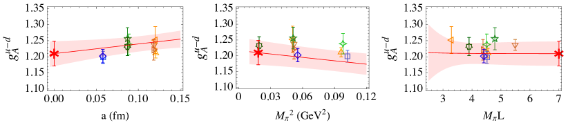
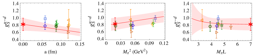
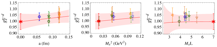
Figure 2: Simultaneous fits in $a$, $M_{\pi}$ and $M_{\pi}L$ using Eq. (3) to obtain the final results for the isovector charges $g_{A}^{u-d}$, $g_{S}^{u-d}$ and $g_{T}^{u-d}$.

Prognosis for 2% estimates: Based on our current analyses, we conclude that to extract $g_{A}$ and $g_{T}$ with $2\%$ uncertainty will require $O(2000)$ configurations with $O(200,000)$ measurements on each of the HISQ ensembles at $a=0.09,0.06$ and $0.045$ fm. Estimates of $g_{S}$ with similar precision will require an order of magnitude more measurements. Equivalently, Clover ensembles at $a=0.09$ 0.07 and $0.05$ fm with similar values of $M_{\pi}\approx 300$, 200 and 140 MeV and $M_{\pi}L\geq 4$ would be needed. These are being generated by the JLab/W&M lattice group.

5 BSM contributions to Neutron Electric Dipole Moment

To explain weak-scale baryogenesis requires CP violation much larger than present in the CKM matrix in the standard model. Most BSM theories have additional sources of CP violation. In an effective field theory formulation, the leading new operators that arise and contribute to the EDM are the quark EDM $d_{q}\ \bar{q}\sigma_{\mu\nu}\gamma_{5}F^{\mu\nu}q$ and the quark chromo EDM $d_{q}\ \bar{q}\sigma_{\mu\nu}\gamma_{5}{\tilde{G}}^{\mu\nu}q$ [9]. The quark EDM contribution of the light $u,d,s$ quarks to the neutron EDM $d_{n}$ is then given by

$$d_{n}=d_{u}g_{T}^{u}+d_{d}g_{T}^{d}+d_{s}g_{T}^{s}\,.$$ (5)

$d_{q}$ are the quark EDM induced in BSM theories and run down to the low energy hadronic scale 2 GeV in the $\overline{MS}$ scheme. The flavor diagonal tensor charges $g_{T}^{q}$, calculated using lattice QCD, are also renormalized at the same point. The product $d_{n}$ is, therefore, scale and scheme independent. The calculation of the connected part of $g_{T}^{q}$ is the same as for isovector charges. Estimates of the disconnected contribution, obtained using the AMA method in [2], have large errors and are consistent with zero. For $g_{T}^{u}$ and $g_{T}^{d}$ we take the largest value on the five ensembles simulated and add it as an additional error in the connected contribution. Estimates of $g_{T}^{s}$ are also consistent with zero, however, in this case we were able to extrapolate to the continuum limit. Using our results for the neutron [2] (note the quark label interchange $u\leftrightarrow d$ between the neutron and proton)

$$g_{T}^{u}= -0.233(28)\,,$$

$$g_{T}^{d}= 0.774(66)\,,$$

$$g_{T}^{s}= 0.008(9)\,,$$ (6)

and the current bound $d_{n}<2.9\times 10^{-26}e$ cm, the bounds on $d_{u}$ and $d_{d}$ are shown in Fig. 3 (left) [8].

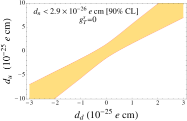
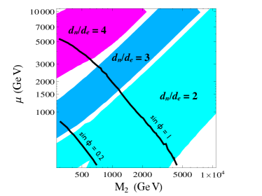
Figure 3: (Left) Allowed region of $d_{u}$ and $d_{d}$ using the current bound on the neutron EDM and $g_{T}^{q}$ in Eq. (6). (Right) Regions in $M_{2}$-$\mu$ plane corresponding to $d_{n}/d_{e}=2,3,4$ in split SUSY, obtained by varying $g_{T}^{u,d,s}$ within our estimated uncertainties. The lines correspond to $d_{e}=8.7\times 10^{-29}\,e$ cm for $\sin\phi=0.2,1$.

In general, BSM theories generate a number of CP-violating operators. However, in the “split SUSY” model [10], fermion EDM operators provide the dominant BSM source of CP violation. In this model, all scalars, except for one Higgs doublet, are much heavier than the electroweak scale. This SUSY scenario achieves gauge coupling unification, has a dark matter candidate, and avoids the most stringent constraints associated with flavor and CP observables mediated by one-loop diagrams involving scalar particles. Contributions to fermion EDMs arise at two loops due to CP violating phases in the gaugino-Higgsino sector, while all other operators are highly suppressed [11]. Using our estimates of $g_{T}^{q}$, we updated the analysis following Ref. [11]. For example, in Fig. 3 (right) we show allowed regions in the gaugino ($M_{2}$) and Higgsino ($\mu$) mass parameter space for different $d_{n}/d_{e}=2,3,4$ [8]. In this model, the $d_{q}$ also depend on a phase $\phi$ and a factor ${\rm tan}\,\beta$. Using this analysis and the current 90% C.L. limit on the electron EDM $d_{e}=8.7\times 10^{-29}\,e$ cm, we derived an upper limit for the neutron EDM in split SUSY i.e., $d_{n}<4\times 10^{-28}\,e$ cm. Consequently, an observation of the neutron EDM between the current limit of $3\times 10^{-26}\,e$ cm and $4\times 10^{-28}\,e$ cm would falsify the split-SUSY scenario with gaugino mass unification.

References

- [1] T. Bhattacharya, , Phys.Rev. D85 (2012) 054512.
- [2] T. Bhattacharya, , Phys.Rev. D92 (2015) 094511.
- [3] T. Bhattacharya, , PoS (LATTICE 2012), 179 (2012) and PoS (LATTICE 2013) 299 (2103).
- [4] A. Bazavov, et al., MILC Collaboration, Phys. Rev. D87 (2013) 054505.
- [5] T. Blum, T. Izubuchi, and E. Shintani, Phys.Rev. D88 (2013) 094503
- [6] T. Bhattacharya, , Phys.Rev. D89 (2014) 094502.
- [7] G. Martinelli, et al., Nucl.Phys. B445 (1995) 81; C. Sturm, et al., Phys.Rev. D80 (2009) 014501.
- [8] T. Bhattacharya, et al., arXiv:1506.04196 [hep-lat]
- [9] M. Pospelov and A. Ritz, Annals Phys. 318, (2005) 119. arXiv:hep-ph/0504231.
- [10] N. Arkani-Hamed and S. Dimopoulos, JHEP 0506, (2005) 73. arXiv:hep-th/0405159.
- [11] G. Giudice and A. Romanino, Nucl.Phys. B699 (2004) 65. arXiv:hep-ph/0406088.
- [12] R. Edwards, B. Joo, Chroma Software System for LQCD, Nucl. Phys. Proc. Suppl. 140 (2005) 832