Search for Extremely Metal-poor Galaxies in the Sloan Digital Sky Survey (II):
high electron temperature objects

Abstract

Extremely metal-poor (XMP) galaxies are defined to have gas-phase metallicity smaller than a tenth of the solar value ($12+\log[{\rm O/H}]<7.69$). They are uncommon, chemically and possibly dynamically primitive, with physical conditions characteristic of earlier phases of the Universe. We search for new XMPs in the Sloan Digital Sky Survey (SDSS) in a work that complements Paper I. This time high electron temperature objects are selected; since metals are a main coolant of the gas, metal-poor objects contain high-temperature gas. Using the algorithm k-means, we classify 788677 spectra to select 1281 galaxies having particularly intense [OIII]$\lambda$4363 with respect to [OIII]$\lambda$5007, which is a proxy for high electron temperature. The metallicity of these candidates was computed using a hybrid technique consistent with the direct method, rendering 196 XMPs. A less restrictive noise constraint provides a larger set with 332 candidates. Both lists are provided in electronic format. The selected XMP sample have mean stellar mass around $10^{8}\,{\rm M}_{\odot}$, with dust-mass $\sim 10^{3}{\rm M}_{\odot}$ for typical star-forming regions. In agreement with previous findings, XMPs show a tendency to be tadpole-like or cometary. Their underlying stellar continuum corresponds to a fairly young stellar population ($<1\,{\rm Gyr}$), although young and aged stellar populations co-exists at the low-metallicity starbursts. About 10 % of the XMPs shows large N/O. Based on their location in constrained cosmological numerical simulations, XMPs have a strong tendency to appear in voids and to avoid galaxy clusters. The puzzling 2 %-solar low-metallicity threshold exhibited by XMPs remains.

1. Introduction

Extremely metal-poor (XMP) galaxies are defined to have a gas-phase metallicity ten times smaller than the sun (e.g., Kunth & Östlin 2000). Even though the exact threshold is arbitrary, this definition selects chemical unevolved galaxies thus providing a gateway to study physical processes in conditions characteristic of the early Universe, which are now unusual. XMPs have been used to determine the primordial He abundance produced during the big bang (Peimbert et al. 2010; Steigman 2010), to study the star-formation in conditions of low metallicity (Shi et al. 2014; Filho 2015b), to infer the formation of dust in the early Universe (Fisher et al. 2014), to analyze properties of a primitive inter-stellar medium (Izotov & Thuan 2007), or to constrain the properties of the first stars (Thuan & Izotov 2005; Kehrig et al. 2015). XMP galaxies are not primeval, but galaxies with an underlying evolved stellar population (e.g., Aloisi et al. 2007; Corbin et al. 2008; Pérez-Montero et al. 2010; Annibali et al. 2013) that look young because they may have recently accreted metal-poor gas (Östlin et al. 2001; Ekta & Chengalur 2010; Sánchez Almeida et al. 2013b, 2014b, 2015), similar to the cold-flows predicted by the numerical simulations of galaxy formation (Dekel et al. 2009; Schaye et al. 2010; Sánchez Almeida et al. 2014a; Nuza et al. 2014b). Then the gas forming stars in XMPs would trace the cosmic web in their immediate surrounding, providing a method to study and to characterize this elusive component of the cosmic web.

Given the general interest and the potential of XMPs as astronomical tools, there have been many attempts to look for new candidates, i.e., to enlarge the list of XMPs, but also to find the least metallic object in the local Universe. However, despite the unquestionable success in finding new objects, the club of XMPs is still quite exclusive. The review paper by Kunth & Östlin (2000) contains only 31 targets, Kniazev et al. (2003) add 8 new targets from the early data release of SDSS, the search in SDSS-DR6 by Guseva et al. (2009) yields 44, and the systematic bibliographic search for all XMPs in the literature carried out by Morales-Luis et al. (2011a, hereinafter Paper I) renders 140. (Paper I includes targets found by Kniazev et al. 2004, Izotov et al. 2004, Izotov et al. 2006, and Izotov & Thuan 2007.) New local metal-poor objects have been discovered since the publication of Paper I (e.g., Izotov et al. 2012; Skillman et al. 2013; James et al. 2015; Guseva et al. 2015), but the situation has not changed in essence. Moreover, even though the number of members of the club has increased since the discovery of IZw18 45 years ago (Sargent & Searle 1970; Searle & Sargent 1972), its low metallicity has not been superseded; the present record-breaking object SBS 0335-052W (Izotov et al. 2009) has a metallicity close to that of IZw18 and around 2 % of the solar value. The existence of such a lower limit for the metallicity of the XMPs has challenged interpretation for decades (e.g., Kunth & Lebouteiller 2011).

The low number of observed XMPs poses a problem since XMPs are expected to be the most common galaxies in the local universe. Because of the luminosity-metallicity relationship (e.g., Skillman et al. 1989; Lee et al. 2006), all galaxies fainter than absolute magnitude ${\rm M}_{B}\simeq-12.5$ are expected to be XMPs (Berg et al. 2012). The extrapolation of the observed galaxy luminosity function to the faint end implies that these ultra-faint XMPs should be the most numerous galaxies in the local universe (e.g., Blanton et al. 2005; Loveday et al. 2015). The reason why these objects are not detected in large quantities seems to be an observational bias, associated with the fact that they are both faint and of low surface brightness. Only when they undergo a starburst phase, brightness and surface density increase to make them detectable in typical magnitude-limited optical surveys (see Skillman et al. 2013; James et al. 2015, and references therein). In order to explain the supposed lack of XMPs, Skillman et al. (2013) proposed the existence of two classes of XMPs: (1) the faint, low surface brightness, quiescent XMPs, very numerous but usually undetected, and (2) the bursting XMPs, going through a transit starburst which allow them to appear in optical surveys like the Sloan Digital Sky Survey analyzed here (Stoughton et al. 2002). Unless otherwise explicitly stated, this paper refers to the latter, even though we often call them XMPs for simplicity. We will mention the class of quiescent XMPs in connection with the number density estimate in Sect. 4.4.

With a few exceptions, the observed XMPs are bursting XMPs, that makes them blue and compact when the star-forming region is large with respect to the size of the galaxy (Kunth & Östlin 2000). Thus bursting XMPs tend to be blue compact dwarf (BCD) galaxies. Their optical spectrum is characterized by intense emission lines (e.g., Terlevich et al. 1991). Many of these XMPs have cometary or tadpole morphology (Papaderos et al. 2008, Paper I). XMP galaxies are gas rich, with a typical gas-mass to stellar-mass ratio in excess of 10 (Filho et al. 2013). They tend to be in relative isolation, although some of them show loose companions. They prefer low density environments identified as voids and sheets in cosmological numerical simulations (Filho et al. 2015).

One of the difficulties to enlarge the sample of XMPs is related to the determination of their chemical abundances, which critically depends on the available optical emission lines. The most accurate method relies on measuring electron temperatures, and uses weak and near-UV emission lines often unavailable. In addition, tailored data-mining techniques are required to identify them since XMPs appear as rare objects in very large surveys. Here we report a new systematic search for XMP galaxies in the Sloan Digital Sky Survey (SDSS-DR7; Abazajian et al. 2009) that overcomes the two aforementioned difficulties. The philosophy remains very much like in Paper I. We carry out an automated classification of the SDSS spectra using k-means (e.g., Sánchez Almeida et al. 2010; Ordovás-Pascual & Sánchez Almeida 2014) in a range of wavelengths particularly sensitive to metallicity. One or a few classes have spectra characteristics of low-metallicity galaxies. Then we measure individually the metallicity of the objects in these classes, so as to confirm or discard these XMP candidates as true members of the XMP party. The difference between Paper I  and the present work is in the wavelength region chosen to classify the spectra. In Paper I  we used the region around H$\alpha$, where the two [NII] lines tend to disappear when the metallicity goes to zero (e.g., Pettini & Pagel 2004; Sánchez Almeida et al. 2012). However, even objects with significant [NII] can be XMP (Morales-Luis et al. 2014), because depending on the evolutionary state and chemical history galaxies may have enhanced N/O, thus presenting large [NII] for a given O (e.g., Pérez-Montero & Contini 2009). Here we use the region between the lines [OIII]$\lambda$4363 and [OIII]$\lambda$5007 which is known to depend on the temperature of the HII region producing the emission-line spectrum. Since metals are a main coolant agent of the gas (e.g., Pagel et al. 1979), metal-poor objects are also high-temperature objects, yielding a relationship between electron temperature and metallicity. This approach is similar to the one already used by Ly et al. (2015), except that they employ it to search for galaxies at a redshift around 0.8, so that the wavelength region of [OIII] is observed in the near IR.

The paper is organized as follows. First, we describe the automated search for XMP candidates using k-means (Sect. 2). It leads to 1281 candidates. Then, we use the SDSS spectra of the candidates to measure their integrated metallicity, which narrows down the list to 196 XMPs (Sect. 3). Emission line fluxes and abundances are calculated in Sects. 3.1 and 3.2, respectively. The final list with 196 XMPs is worked out in Sect. 3.3 (Table 1), where we also include a second list (Table 2) with 332 potential XMPs selected under less restrictive noise constraints. The global properties of the XMPs are analyzed in Sect. 4, explicitly, stellar mass (Sect. 4.2), reddening and dust mass (Sect. 4.1), absolute magnitude and color (Sect. 4.3), number density (Sect. 4.4), metallicity threshold (Sect. 4.5), morphology (Sect. 4.6), underlying stellar population (Sect. 4.7), and large scale environment (Sect. 4.8). The results are summarized and discussed in Sect. 5. The number of false positives and false negatives in Table 1 is estimated in Appendix A.

2. Search for XMP candidates classifying the spectrum around [OIII]$\lambda$4363

The ratio between the emission of [OIII]$\lambda$4363 and the pair [OIII]$\lambda\lambda$4959,5007 strongly depends on the metallicity of the emitting gas. The reason is well known and rather straight-forward. Since metals are a main coolant of the gas (e.g., Pagel et al. 1979), metal-poor gas is also high-temperature gas. The ratio [OIII]$\lambda$4363 to [OIII]$\lambda\lambda$4959,5007 is used to measure [OIII] electron temperature in HII regions (e.g., Hägele et al. 2008), therefore it is also a good proxy for metallicity. The three [OIII] lines are excited by collisions with free electrons, and their decay through photon emission renders the observed lines. The excitation potential of the upper level of [OIII]$\lambda$4363 (${}^{1}{\rm S}_{0}$; $5.35$ eV) is significantly higher than the upper level shared by [OIII]$\lambda$4959 and [OIII]$\lambda$5007 (${}^{1}{\rm D}_{2}$; $2.51$ eV), so that [OIII]$\lambda$4363 increases relative to the other two lines as the temperature increases, that is to say, as the metallicity of the gas decreases. The relative fluxes change by more than one order of magnitude when the electron temperature changes in the range of the typical temperatures in HII regions, say, between 5 and 25 kK (e.g., Osterbrock 1974).

We take advantage of this sensitivity of the spectrum on metallicity to search for XMP candidates. Using the automatic classification algorithm k-means (Sánchez Almeida et al. 2010; Ordovás-Pascual & Sánchez Almeida 2014), we classify the full SDSS-DR7 spectral database according to the shape of the spectrum of the galaxies in the spectral region of interest, from 4200 to 5200 Å, which contains [OIII]$\lambda$4363, [OIII]$\lambda$4959, and [OIII]$\lambda$5007. As in Paper I, the signal to be classified, $S(\lambda)$, is the observed spectrum in rest-frame wavelength, $I(\lambda)$, after removing the continuum intensity, $I_{c}(\lambda)$, and after the subsequent normalization to the emission at the reference wavelength (4363 Å in this case), explicitly,

$$S(\lambda)={{I(\lambda)-I_{c}(\lambda)}\over{I(4363\,{\rm\AA})-I_{c}(4363\,{\rm\AA})}}.$$ (1)

We start from the full set of 788677 galaxy spectra from SDSS-DR7 having redshift smaller than 0.25 (Sánchez Almeida et al. 2010). The classification renders 17 types or classes. The two of them showing the largest [OIII]$\lambda$4363, which include 24200 objects, are re-classified to obtain 12 subclasses. Some of these subclasses collect noisy spectrum, and those are discarded so that k-means acts as a noise filter. Four of the subclasses show particularly intense [OIII]$\lambda$4363, as depicted in Fig. 1. (Note that, even in these cases, the flux of [OIII]$\lambda$4363 is much smaller than the fluxes of [OIII]$\lambda$4959, [OIII]$\lambda$5007 – the spectra in Fig. 1 have [OIII]$\lambda$5007 some fifty times larger than [OIII]$\lambda$4363.) Classes #8 and #11 in Fig. 1 are discarded because the mean spectrum of the class appears in the region of Active Galactic Nuclei (AGNs) of the BPT diagram (Baldwin et al. 1981; Sánchez Almeida et al. 2012). Therefore, their high excitation is produced by hard AGN radiation, rather than by lack of efficient coolants in a stellar-radiation excited HII region. The AGN nature of the discarded classes is corroborated by the large width of their emission lines (cf. AGN classes, #8 and #11, with star-forming classes #4 and #6), a property also characteristic of AGNs. After the classification and trimming, we are left with 1281 bursting XMP candidates.

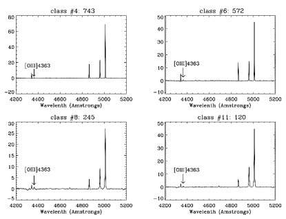
Figure 1.— Template of four spectral classes where the emission line [OIII]$\lambda$4363 (marked with arrows) is particularly intense compared to [OIII]$\lambda$4959 and [OIII]$\lambda$5007. They were found by applying two nested k-means classifications to the 788677 galaxies with spectra in SDSS-DR7 having redshift $<0.25$. Two of the classes ( #8 and #11) are AGNs, as proven by their position on the BTP diagram and the fact that the emission lines are particularly broad. The spectra, with the continua removed, have been normalized to the peak intensity of [OIII]$\lambda$4363. Wavelengths are given in Å. The label on top of each panel represent the class number and the number of galaxies in the class.

We have compared these 1281 candidates with the 32 XMPs selected in Paper I after classifying the spectral region around H$\alpha$. Most of them, 29 out of the 32, are included in our list of candidates. Considering that the two procedures are completely independent, and the randomness inherent to the k-means procedure, the agreement is very reasonable. Recall that k-means is a powerful tool able to classify very large data sets in high-dimensional spaces. However, among its drawbacks, k-means does not provide a single classification for a single database. Each particular run depends on a random initialization, thus, the classification is not unique (e.g., Sánchez Almeida et al. 2010, Sect. 2).

Nothing ensures that the 1281 candidates are true XMPs. They have been picked up as objects where [OIII]$\lambda$4363 is particularly intense, using as reference the rest of galaxies in the spectroscopic database of SDSS-DR7. In order to show whether or not they are XMPs, we have computed the metallicity for every one of them to mark as XMP only those objects of truly low metallicity. (The details are given in the next Sect. 3.) One may think of this second step as a way to clean from pollutants the systematic but otherwise rough XMP selection carried out by k-means on the SDSS-DR7 database.

3. Metallicities of the XMP candidates

3.1. Determination of emission line fluxes

We use the SDSS-DR7 spectra of the 1281 candidates to determine their metallicities. As usual, the procedure requires correcting the emission line fluxes for reddening, which is determined from the relative fluxes of the observed Balmer lines (e.g., Hägele et al. 2008; Stasińska et al. 2012). However, Balmer emission is usually depressed due to the presence of absorption lines of stellar origin. Therefore, prior to the measurement of the emission lines, we perform a stellar fitting to the continuum of the spectra. We use starlight (Cid Fernandes et al. 2005) to model the spectral energy distribution (SED) of the underlying stellar population. Starlight fits the observed continuum as a linear combination of single stellar population (SSP) spectra of various ages and metallicities. We chose the SSP spectra from Bruzual & Charlot (2003), including four metallicities $Z=0.0001,0.0004,0.004,$ and 0.008 (1%, 3%, 30% and 60% $Z_{\odot}$, respectively; Asplund et al. 2009). Reddening of the stellar SED was included assuming the extinction to follow Cardelli et al. (1989) with $R_{V}$ = 3.1. The stellar continuum thus obtained is subtracted out of the observed spectrum to produce a pure emission line spectrum. The latter is employed to determine line fluxes.

We used the package shifu to obtain the flux of the emission lines. The package contains a suite of routines to easily analyze emission or absorption lines in IFU data (both in cube and RSS format). Individual spectra, such as those employed in our particular case, can be provided as a list of files (RSS). The core of the code uses CIAO’s Sherpa package (Freeman et al. 2001; Doe et al. 2007). Several custom algorithms are implemented in order to cope with general and ill-defined cases. A sigma-clipping is independently applied to the stellar continuum model, and then this is parsed to the composite line plus continuum model. Although the fitting is performed in the residual spectra, we allow for the modeling of the continuum to take into account small deviations in the stellar continnum residuals. A first order polynomial has been chosen for the continuum, while single gaussians have been selected for the lines. The continuum is evaluated in the original spectra when used to determine equivalent widths.

3.2. Method to measure metal abundance

Metal abundances are computed with the code HII-CHI-mistry (hereafter HCM Pérez-Montero 2014), which calculates the total oxygen abundance O/H, the nitrogen-to-oxygen ratio N/O, and the ionization parameter U. Normalized to H$\beta$ and corrected for extinction, the fluxes of the emission lines [OII]$\lambda$3727, [OIII]$\lambda\lambda$4363,5007, [NII]$\lambda$6584, and [SII]$\lambda\lambda$6716,6731 are compared with the predictions of a large grid of cloudy (Ferland et al. 2013) photoionization models. The HCM assumes a spherically symmetric constant-density distribution of gas ionized by popstar (Mollá et al. 2009) 1 Myr-old stellar clusters with the same metallicity of the gas, and covering a wide range of values in O/H, N/O, and log U. In particular, the grid includes very low values of the gas metallicity, down to 12+log(O/H)=6.9 equivalent to 1/60 of the oxygen abundance in the solar composition (Asplund et al. 2009). The main advantage of this method is that it leads to a derivation of the chemical abundances consistent with the direct method even in the absence of one or more of the input emission lines (Pérez-Montero 2014). Since the direct method does not depend on modeling (e.g., Osterbrock 1974; Stasińska et al. 2012), it means that the metallicities provided by HCM are almost insensitive to the model assumptions. Given a set of observed line ratios, HCM assigns a $\chi^{2}$ to each one of the models, computed as the sum of the square differences between the observed and the model line ratios. The $1/\chi^{2}$-weighted average of the abundance in the models yields the chemical abundance tagged to the observed line ratios. Errors are derived as the $1/\chi^{2}$-weighted standard deviation of the parameters in the models. When the temperature-sensitive line [OIII]$\lambda$4363 is available, HCM uses the whole grid of models to provide values of O/H and N/O that are consistent with the direct method, even in the absence of [OII]$\lambda$3727. Thus the use of HCM results especially appropriate to search for XMPs in SDSS since [OII]$\lambda$3727 is sometimes outside the observed spectral region for nearby objects. The error bars estimated by HCM quantify the internal precision of the method, i.e., they give the range of models that is consistent with the observed line fluxes. The observational errors enter into the abundance error estimate indirectly, since the observed fluxes must have enough signal to be considered for analysis.

3.3. List of XMPs

The automated procedure described in Sect. 3.1 provides the fluxes used by HCM (Sect. 3.2) to infer the oxygen abundance of the 1281 candidates (Sect. 2). We consider only line fluxes with a signal-to-noise ratio larger than three, including the weak [OIII]$\lambda$4363. The scatter plot 12+log(O/H) vs log(N/O) for the full sample is shown in Fig. 2a. Assuming that the solar composition corresponds to 12+log(O/H)${}_{\odot}\simeq 8.69$ (Asplund et al. 2009), XMPs are defined as those candidates having

$$12+\log({\rm O/H})\leq 7.69.$$ (2)

There are 196 galaxies fulfilling this requirement, which are the bursting XMP galaxies presented in this work. 11 of them have duplicated spectra in SDSS-DR7. We have chosen for analysis the spectrum yielding the smallest error in metallicity. The XMP galaxies are represented as red squares with error bars in Fig. 2a. The distribution of metallicities of the candidates is given in Fig. 2b. The histogram is fairly continuous at the border between XMPs and the rest, which proves the 1/10 solar metallicity threshold to be rather arbitrary.

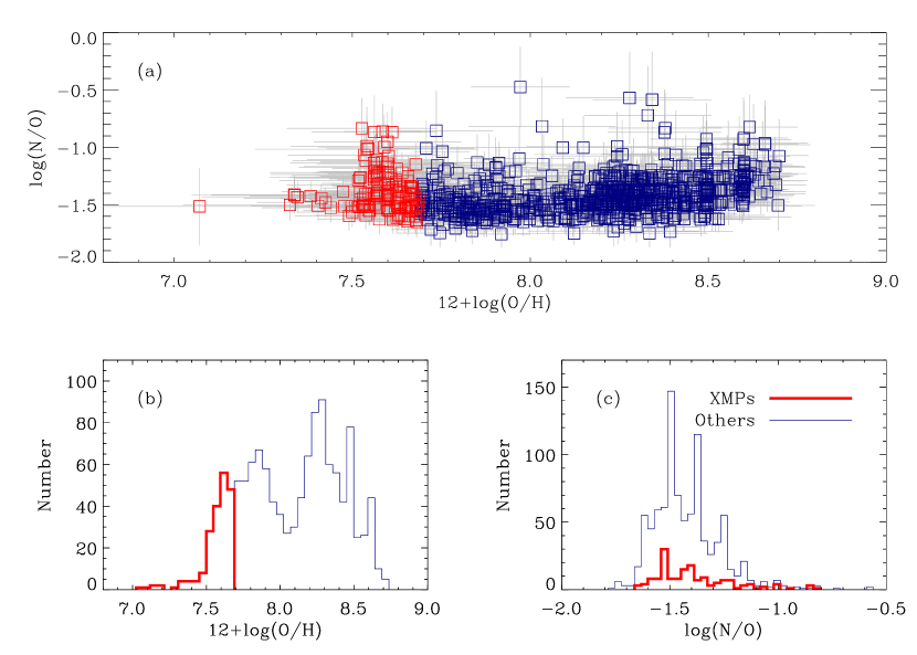
Figure 2.— (a) Scatter plot N/O vs O/H for the XMPs found in our search (red squares with error bars), and for the candidates that turned out not to be XMPs (blue symbols with error bars). (b) Distribution of the O abundance for the XMPs (thick red line) and the failed candidates (thin blue line). It is rather smooth at the transition abundance (7.69, equivalent to a tenth of the solar value). (c) Distribution of N/O for the XMPs (thick red line) and the rest (thin blue line).

The list of XMPs is given in Table 1, which includes coordinates as well as the main physical properties provided by HCM. When [NII]$\lambda$6584 is too weak for the noise level, N/O cannot be derived, and it appears as -9.99 in the Table. The distributions of N/O for the XMPs and the rest of the sample are given in Fig. 2c. They look qualitatively similar.

We carried out several sanity checks. First, we estimated the number of false positives and false negatives due to observational errors. False positives are galaxies in the XMP list which have true oxygen abundance above the threshold. False negatives are true XMP galaxies that have been discarded from the selection. Using a Bayesian approach, we work out in Appendix A the expected number of false positives and false negatives. Even though the typical error of the individual abundance estimates is rather small ($\simeq 0.17$ dex for the galaxies in Table 1), we expect a significant number of false positives and false negatives. Assuming the true distribution of metallicities to be given by the histogram in Fig. 2b, we expect 82 false positives and 46 false negatives (Eq. [A8]). If the true distribution is uniform, then the number of both false positives and false negatives is around 55 (Eq. [A9]). Partly to offer the possibility of recovering false negatives in the future, we include a 2nd list with candidate XMPs in Table 2. Table 1 is based on lines with measured fluxes exceeding three times the noise. If this threshold is lowered, and lines with fluxes at two-sigma are also considered, then the number of galaxies fulfilling the condition in Eq. (2) increases to 332, and those are the objects included in Table 2. The reason why the number increases when lowering noise limit can be pinned down to the weakness of [OIII]$\lambda$4363, which tends to be excluded from the metallicity estimate when the noise limit is too restrictive. When it is considered in the metallicity estimate, HCM tends to lower the oxygen abundance estimate due to arguments given in Sect. 2

As a second test, we compared the metallicity provided by HCM with the metallicity obtained with the direct method (e.g., Hägele et al. 2008) when [OII]$\lambda$3727 was available . These abundances, based on the direct method, are also included in Table 1. The scatter plot direct-method metallicity vs HCM metallicity is shown in Fig. 3. As expected, the two techniques agree quite well with a dispersion of only 0.04 dex, which is smaller than the intrinsic error of both methods. On top of this agreement, there is a tendency for HCM to overestimate the direct-method metallicity at low metallicities. Since this bias occurs below the threshold metallicity to be XMP (Eq. [2]), both methods would yield the same list of XMPs if we had access to [OII]$\lambda$3727. Moreover, the systematic differences between the abundances obtained from HCM and the direct method are small compared with their error bars, so that such differences barely affect other results and conclusions of the paper. For example, adding an extra 0.06 dex error to the typical $\sim 0.17~{}$dex error bar increases the number of false positives worked out in Appendix A, but only from 82 to 86.

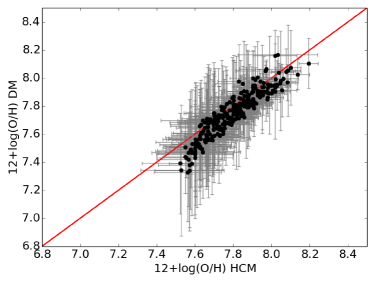
Figure 3.— Scatter plot direct-method metallicity vs HCM metallicity for the galaxies having [OII]$\lambda$3727 within the observed spectral range. Both measurements agree quite well, with a small difference at metallicities below the XMP threshold which consequently does not affect the selection of XMPs. The solid line corresponds to the one-to-one relationship.

As a final test, we represented our targets in the [OIII]$\lambda$5007/H$\beta$ vs [NII]$\lambda$6583/H$\alpha$ plane commonly used to separate starbursts from AGNs (the so-called BPT diagram, after Baldwin et al. 1981); see Fig. 4. None of them are AGNs, and only two reside in the composite-spectrum region next to the divide worked out by Kauffmann et al. (2003). They may be starbursts of high N/O (Pérez-Montero & Contini 2009), or HII regions where the excitation may have contribution from shocks, evolved stars, or even AGNs. The two objects with composite-spectrum are number 51 and number 151 in Table 1, and their identification as XMP galaxies must be taken with caution.

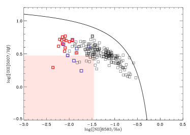
Figure 4.— Scatter plot [OIII]$\lambda$5007/H$\beta$ vs [NII]$\lambda$6583/H$\alpha$ for the galaxies in Table 1. This plane is commonly used to separate starbursts from AGNs (the so-called BPT diagram, after Baldwin et al. 1981). Most objects reside below the solid line by Kauffmann et al. (2003), corresponding to excitation by stars. Only two objects are close to this border and they may have composite spectra. The shaded region shows the area used by Izotov et al. (2012) to search for XMPs in SDSS-DR7. The colored points correspond to objects also found in Paper I (red) and in Izotov et al. (2012, blue). Contrarily to our targets, these previous searches pick up emitters concentrated on the leftmost region of the BPT diagram, corresponding to [NII]$\lambda$6583$\ll$H$\alpha$.

Most of the 196 galaxies in Table 1 seem to be new members of the XMP class. Table 2 of Paper I compiles all XMPs in the literature up to the date of publication in mid 2011. It contains 129 objects, 21 of which coincide with objects in Table 1. Paper I also carries out a systematic search for XMPs in SDSS-DR7, finding 32 such objects. 17 of these 32 targets coincide with targets selected in our study, and so are included in Table 1. In addition, there is a recent major search for XMPs by Izotov et al. (2012), which contains 41 targets. Among them, 7 are in Table 1. Considering all the objects in these three lists, and discarding coincidences, only 31 among the 196 galaxies in Table 1 seem to be known. Known and unknown targets are pointed out in one of the columns of Table 1, which used the following code to indicate matches: (1) Table 1 in Paper I, (2) Table 2 in Paper I, (3) Tables 1 & 2 in Paper I, (4) Izotov et al. (2012), (5) Table 1 in Paper I  & Izotov et al. (2012), (6) Table 2 in Paper I  & Izotov et al. (2012), (7) Table 1 & 2 in Paper I, & Izotov et al. (2012), and finally, (0) no match.

Part of the difference with previous searches is related to the abundance threshold (Eq. [2]). Our criterion is slightly less restrictive than others (see footnote number 3) therefore, by construction, the highest metallicity targets in Table 1 are discarded in other compilations. For example, 43 and 88 objects have $12+\log({\rm O/H})>7.65$ and $>7.60$, respectively. In addition to this fact, however, we employ a novel selection procedure which influences the results. Figure 4 provides the clue for understanding the main difference between our search and previous ones. Previous searches are focused on objects having small [NII]$\lambda$6583 compared with H$\alpha$ (Paper I) or with H$\beta$ (e.g., Izotov & Thuan 2007; Izotov et al. 2012), whereas our technique selects objects that cover a significant part of the BPT plane. XMP galaxies of relatively large [NII]$\lambda$6583/H$\alpha$ are know to exist due to, e.g., having particularly large N/O or displaying particularly low ionization (e.g., Morales-Luis et al. 2014). Our approach is sensitive to those XMPs, as it is evidenced in Fig. 4, which shows with colored symbols the objects in common with the searches in Paper I and Izotov et al. (2012). The region explored by (Izotov et al. 2012) is also indicated in the figure.

The histogram of metallicities in Fig. 2a drops at $12+\log({\rm O/H})\leq 7.50$, so that only 28 of the XMPs in Table 1 have oxygen abundance smaller than this threshold. (The lowest metallicity limit is discussed in Sect. 4.5.) Those objects are particularly rare, here and in previous works (e.g., Paper I; Izotov et al. 2012; Guseva et al. 2015), however, this part of Table 1 is the one that contains more targets in common with previous searches. Actually, 36 % of our XMPs with $12+\log({\rm O/H})\leq 7.50$ are already known, whereas the 31 known objects in Table 1 represent only 16% of the full list of 196 targets.

Table 1Extremely metal poor galaxies selected in this study

Index	Name	12+log(O/H)	log(N/O)	logU	CH$\beta$	Match	12+log(O/H)DM
1	J$001637.4+003828.8$	7.66$\pm$0.18	-1.60$\pm$0.14	-2.65$\pm$0.12	0.00$\pm$0.04	0	7.59$\pm$0.19
2	J$001922.9-002450.5$	7.57$\pm$0.19	-1.11$\pm$0.23	-2.54$\pm$0.16	0.27$\pm$0.03	0	7.47$\pm$0.18
3	J$002114.8-085809.5$	7.56$\pm$0.23	-1.14$\pm$0.28	-2.65$\pm$0.19	0.62$\pm$0.01	0	9.99$\pm$0.00
4	J$002916.8-010021.2$	7.61$\pm$0.16	-1.35$\pm$0.15	-2.04$\pm$0.33	0.17$\pm$0.02	0	9.99$\pm$0.00
5	J$003630.4+005234.7$	7.58$\pm$0.12	-9.99$\pm$0.00	-1.88$\pm$0.25	0.01$\pm$0.03	1	7.39$\pm$0.08
6	J$003741.1+003320.1$	7.68$\pm$0.12	-1.52$\pm$0.13	-1.89$\pm$0.27	0.00$\pm$0.03	0	9.99$\pm$0.00
7	J$004224.8+003315.7$	7.63$\pm$0.16	-1.51$\pm$0.14	-2.55$\pm$0.18	0.07$\pm$0.03	0	9.99$\pm$0.00
8	J$005249.8-084133.9$	7.63$\pm$0.15	-1.48$\pm$0.15	-2.66$\pm$0.21	0.23$\pm$0.03	0	9.99$\pm$0.00
9	J$011914.3-093546.2$	7.60$\pm$0.14	-1.55$\pm$0.12	-1.92$\pm$0.27	0.15$\pm$0.02	2	9.99$\pm$0.00
10	J$013352.6+134209.4$	7.46$\pm$0.14	-9.99$\pm$0.00	-1.79$\pm$0.23	0.26$\pm$0.03	2	9.99$\pm$0.00
11	J$015759.7+011138.6$	7.56$\pm$0.29	-1.22$\pm$0.20	-2.65$\pm$0.13	0.11$\pm$0.05	0	9.99$\pm$0.00
12	J$022107.2-002507.3$	7.60$\pm$0.20	-1.41$\pm$0.16	-2.53$\pm$0.19	0.15$\pm$0.02	0	9.99$\pm$0.00
13	J$022237.8+002908.0$	7.67$\pm$0.15	-1.56$\pm$0.13	-2.54$\pm$0.17	0.28$\pm$0.05	0	9.99$\pm$0.00
14	J$022607.0+000017.7$	7.64$\pm$0.20	-1.39$\pm$0.17	-2.56$\pm$0.17	0.04$\pm$0.02	0	9.99$\pm$0.00
15	J$024223.6-005817.3$	7.66$\pm$0.12	-1.29$\pm$0.16	-1.78$\pm$0.19	0.21$\pm$0.02	0	7.54$\pm$0.17
16	J$024429.0+000741.4$	7.55$\pm$0.12	-1.01$\pm$0.00	-1.64$\pm$0.18	0.00$\pm$0.06	0	9.99$\pm$0.00
17	J$024636.4+001654.9$	7.60$\pm$0.20	-1.42$\pm$0.16	-2.53$\pm$0.19	0.30$\pm$1.27	0	9.99$\pm$0.00
18	J$025818.9+004348.7$	7.60$\pm$0.24	-1.41$\pm$0.18	-2.53$\pm$0.18	0.26$\pm$0.01	0	9.99$\pm$0.00
19	J$030149.0-005257.4$	7.58$\pm$0.12	-9.99$\pm$0.00	-1.86$\pm$0.24	0.29$\pm$0.04	2	9.99$\pm$0.00
20	J$031137.9-003332.0$	7.58$\pm$0.13	-9.99$\pm$0.00	-2.38$\pm$0.20	0.19$\pm$0.01	0	9.99$\pm$0.00
⋮	⋮	⋮	⋮	⋮	⋮	⋮	⋮

Table 2Candidate XMP galaxies

Index	Name	12+log(O/H)	log(N/O)	logU	CH$\beta$
1	J$000009.0+011423.8$	7.67$\pm$0.18	-1.44$\pm$0.15	-2.58$\pm$0.13	0.29$\pm$0.06
2	J$001432.7+002919.9$	7.60$\pm$0.24	-1.37$\pm$0.22	-2.63$\pm$0.12	0.09$\pm$0.03
3	J$001637.4+003828.8$	7.66$\pm$0.18	-1.60$\pm$0.14	-2.65$\pm$0.12	0.00$\pm$0.04
4	J$001922.9-002450.5$	7.57$\pm$0.19	-1.11$\pm$0.23	-2.54$\pm$0.16	0.27$\pm$0.03
5	J$002114.8-085809.5$	7.56$\pm$0.23	-1.14$\pm$0.28	-2.65$\pm$0.19	0.62$\pm$0.01
6	J$002535.1+003456.1$	7.61$\pm$0.18	-1.27$\pm$0.24	-2.68$\pm$0.21	0.15$\pm$0.04
7	J$002916.8-010021.2$	7.61$\pm$0.16	-1.35$\pm$0.15	-2.04$\pm$0.33	0.17$\pm$0.02
8	J$003145.3-110656.8$	7.61$\pm$0.17	-1.56$\pm$0.12	-2.24$\pm$0.33	0.13$\pm$0.18
9	J$003630.4+005234.7$	7.59$\pm$0.12	-1.51$\pm$0.14	-1.89$\pm$0.25	0.01$\pm$0.03
10	J$003741.1+003320.1$	7.68$\pm$0.12	-1.52$\pm$0.13	-1.89$\pm$0.27	0.00$\pm$0.03
11	J$004224.8+003315.7$	7.63$\pm$0.16	-1.51$\pm$0.14	-2.55$\pm$0.18	0.07$\pm$0.03
12	J$004521.9-093700.1$	7.52$\pm$0.21	-1.44$\pm$0.13	-1.92$\pm$0.43	0.09$\pm$0.03
13	J$004614.4+000635.9$	7.55$\pm$0.20	-1.28$\pm$0.25	-2.50$\pm$0.19	0.25$\pm$0.03
14	J$005249.8-084133.9$	7.63$\pm$0.15	-1.48$\pm$0.15	-2.66$\pm$0.21	0.23$\pm$0.03
15	J$010408.4-004010.3$	7.60$\pm$0.15	-1.38$\pm$0.16	-2.38$\pm$0.17	0.21$\pm$0.12
16	J$010413.3+001529.0$	7.56$\pm$0.21	-1.20$\pm$0.22	-2.65$\pm$0.13	0.16$\pm$0.04
17	J$010414.6-005040.1$	7.31$\pm$0.34	-1.38$\pm$0.22	-1.71$\pm$0.32	0.20$\pm$0.04
18	J$011144.5+010929.8$	7.55$\pm$0.22	-1.44$\pm$0.23	-2.41$\pm$0.24	0.09$\pm$0.23
19	J$011340.5+005239.2$	7.04$\pm$0.26	-9.99$\pm$0.00	-1.55$\pm$0.10	0.00$\pm$0.01
20	J$011914.3-093546.2$	7.60$\pm$0.14	-1.55$\pm$0.12	-1.92$\pm$0.27	0.15$\pm$0.02
⋮	⋮	⋮	⋮	⋮	⋮

4. Properties of the XMPs

4.1. Reddening and dust mass

Dust is made out of metals and so metal-poor objects are also expected to be dust-poor (Krumholz 2013; Fisher et al. 2014). However, the type of bursting XMPs selected here are going through a starburst phase where SNe go off continuously creating dust that may potentially obscure the light from the starburst (e.g., Tenorio-Tagle et al. 2013). Consequently, one expects small but non-zero amounts of extinction in XMPs. This is actually the case in our XMP sample.

As a by-product of the metallicity estimate, we have to measure the extinction coefficient that renders the observed Balmer decrement (Sect. 3.1). We follow the procedure described by Hägele et al. (2008), where the shape of the extinction law is taken to be the Milky-Way extinction law by Cardelli et al. (1989). Using the usual parametrization, the extinction coefficient at H$\beta$, c(H$\beta$), is defined to be

$${\rm c(H}\beta)=-\log(F/F_{0}),$$ (3)

where the symbols $F$ and $F_{0}$ stand for the reddened and original fluxes in H$\beta$, respectively. Therefore, the extinction coefficient is proportional to the optical depth along the line-of-sight $\varpi$ (e.g., Osterbrock 1974),

$${\rm c(H\beta)}=\varpi\,\log e,$$

with

$$\varpi=\int_{0}^{l_{0}}\kappa_{D}\,\rho_{D}\,dl.$$ (4)

The integral goes along the line-of-sight from the observer to the source of light at $l_{0}$. The symbols $\rho_{D}$ and $\kappa_{D}$ stand for the dust density and the cross section per unit mass of dust, respectively. Defining the density-weighted mean cross section $\langle\kappa_{D}\rangle$,

$$\langle\kappa_{D}\rangle=\int_{0}^{l_{0}}\kappa_{D}\,\rho_{D}\,dl\Big{/}\int_{0}^{l_{0}}\rho_{D}\,dl,$$ (5)

then the dust-mass column density,

$$\Sigma_{D}=\int_{0}^{l_{0}}\rho_{D}\,dl,$$

can be inferred from the extinction coefficient as

$$\Sigma_{D}={\rm c(H\beta)}/\big{[}\langle\kappa_{D}\rangle\log e\big{]}.$$ (6)

Figures 5a and 5b show scatter plots of extinction versus metallicity and N/O, respectively.

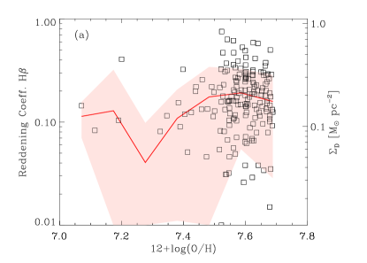
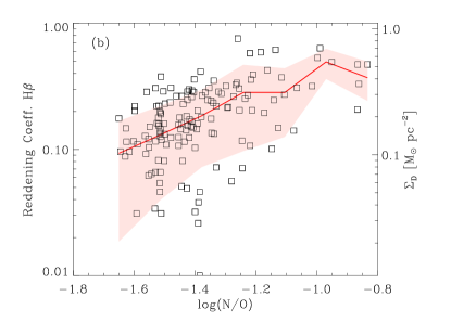
Figure 5.— (a) Extinction coefficient at the wavelength of H$\beta$ versus oxygen abundance. The symbols show individual XMP galaxies whereas the solid line and the shaded region correspond to the mean and the standard deviation of the distribution of points. There is no clear trend. The second ordinate axis portrays the dust column density needed to produce the observed reddening (see text for details). (b) Extinction coefficient at H$\beta$ versus nitrogen over oxygen. The symbols show individual galaxies whereas the solid line and the shaded region correspond to the mean and the standard deviation of the distribution of points. There is a trend, so that the reddening increases with increasing N/O.

We find no clear relationship between extinction and metallicity (Fig. 5a). However, there is a hint of correlation between extinction and log(N/O), so that the larger the ratio between nitrogen and oxygen the larger the reddening (Fig. 5b). The scatter of the possible relationship is large; the extinction coefficient increases only a factor of three over the full range of N/O, and this increase is similar to the dispersion of the individual galaxies in the scatter plot (Fig. 5b).

The ordinate axes on the right of Figs. 5a and 5b quantify the dust-mass column density responsible for the observed extinction. We have used Eq. (6) with a cross-section per unit mass $\langle\kappa_{D}\rangle=10^{4}\,{\rm cm^{2}\,g^{-1}}$, which is representative of this quantity at H$\beta$ (e.g., Draine 2003, Table 4). For the typical size of the giant HII regions in these objects, of the order of 150 pc (e.g., Sánchez Almeida et al. 2013b, 2015), the mass in dust corresponding to the observed surface density spans from 2$\times 10^{2}$ to 2$\times 10^{4}$ ${\rm M_{\odot}}$. For reference, the dust mass of the prototypical XMP IZw 18, as inferred from modeling IR dust emission, is between 450 and 1800 ${\rm M_{\odot}}$ (Fisher et al. 2014). IZw18 is included in Table 1, and its spectrum shows no extinction with an uncertainty of 0.07, which sets an upper limit of 1.5$\times 10^{3}$ ${\rm M_{\odot}}$ consistent with the value inferred from dust emission by Fisher et al.

The distribution of extinction coefficients for the XMPs in Table 1 has a mean and a standard deviation given by

$$\mu_{\rm c(H\beta)}\pm\sigma_{\rm c(H\beta)}=0.17\pm 0.14.$$ (7)

Using Eq. (6), this extinction corresponds to a dust mass column density of,

$$\mu_{\Sigma_{D}}\pm\sigma_{\Sigma_{D}}=(0.19\pm 0.15)\,{\rm M_{\odot}\,pc^{-2}}.$$ (8)

4.2. Stellar masses

Stellar masses are usually estimated from photometry via models that provide the light-to-mass ratio (M/L) given the observed colors of a galaxy (e.g., Bell & de Jong 2001). This procedure is particularly uncertain for bursting XMP galaxies, with spectra having intense emission lines that are hard to capture by the model used for M/L. However, stellar mass is one of the central parameters characterizing galaxies, therefore, even with the above caveat in mind, we have analyzed photometry-based stellar masses of the XMP galaxies. We use those from the Max-Planck-Institute for Astrophysics – Johns Hopkins University (MPA-JHU) characterization of the SDSS-DR7 galaxy spectral data (Brinchmann et al. 2004; Salim et al. 2007). Broad-band galaxy-integrated magnitudes from the SDSS-DR7 database are compared with a grid of theoretical galaxy spectra (Bruzual & Charlot 2003) spanning a large range in star-formation histories (Salim et al. 2007). From the difference between observed and theoretical magnitudes, a likelihood distribution for the mass of each galaxy is estimated. We use the median and the dispersion of this distribution in our analysis.

The observed stellar masses have a mean and a standard deviation of

$$\mu_{\rm\log M_{\star}}\pm\sigma_{\rm\log M_{\star}}=8.0\pm 1.1,$$ (9)

where the masses have been expressed in solar masses. The XMPs are generally dwarfs, but there is a large spread in their possible masses – ${\rm\log(M_{\star}/M_{\odot})}$ spans from 6 to 10. This can be appreciated in Fig. 6, which shows the scatter plot metallicity vs stellar mass.

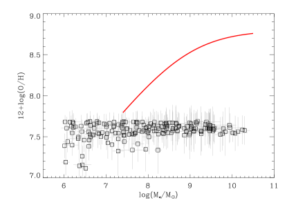
Figure 6.— Metallicity vs stellar-mass scatter plot for the XMPs in Table 1 (the symbols with error bars). Although XMPs tend to be low-mass, there is a large spread in stellar masses. When galaxies are chosen independently of metallicity, their stellar masses and metallicities are related – the solid line represents the mean correlation observed and parameterized by Andrews & Martini (2013). There is no relationship in the case of the XMPs.

f

We find no clear trend for the metallicity to vary with stellar mass. This is forced by the selection criteria imposed on the XMPs. In a randomly chosen set of galaxies, stellar masses and metallicities are correlated (e.g., Tremonti et al. 2004). Such relationship, as updated by Andrews & Martini (2013), is included in Fig. 6. By construction, XMPs are restricted to have low metallicity and therefore cannot follow the general trend dictated by the red solid line in Fig. 6. However, hints of the underlying mass-metallicity relationship remains in the XMP sample, because the lowest abundances are associated with galaxies in the low-mass part of the mass distribution (Fig. 6). Figure 7 shows the scatter plot N/O vs stellar mass. There is a clear trend for N/O to increase with increasing stellar mass for $\log({\rm M}_{\star}/{\rm M}_{\odot})>8.5$, which is consistent with the relationship found in local galaxies (e.g., Pérez-Montero & Contini 2009; Pérez-Montero et al. 2013). In addition, some low-mass XMPs do show large N/O. The combination of low metallicity and high N/O can be understood if these galaxies suffered a major metal-poor gas accretion event that dropped O/H keeping N/O unchanged (see Sect. 5 for more details).

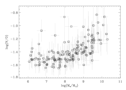
Figure 7.— Scatter plot N/O vs stellar mass for the XMP galaxies in Table 1 (symbols with error bars). There is a clear tendency for N/O to increase with increasing stellar mass when $\log({\rm M}_{\star}/{\rm M}_{\odot})>8.5$.

We also find a correlation between reddening and stellar mass (Fig. 8). It reflects the correlation between N/O and reddening (Fig. 5b), given the fact that N/O increases with increasing stellar mass (Fig. 7).

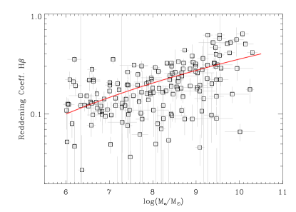
Figure 8.— Scatter plot reddening coefficient vs stellar mass for the XMP galaxies in Table 1 (symbols with error bars). There is a tendency for the reddening to increase with increasing stellar mass, however, the spread of reddening for a given stellar mass is large. The straight line has been included to guide the eye.

We note that none of the large N/O targets have $12+\log({\rm O/H})>7.5$ (Fig. 2a).

4.3. Magnitudes and colors

Figure 9 shows the color magnitude diagram in the color filters $g$ and $r$. We use Petrosian magnitudes of the integrated galaxias as provided by SDSS. The figure includes the color threshold to be a blue compact dwarf galaxy as defined by Gil de Paz et al. (2003) (and transformed from U and B to $g$ and $r$ by Sánchez Almeida et al. 2008). Most XMPs lie below the threshold and thus look blue in broad-band colors. However, a significant part of them are not dwarf, with absolute magnitude in excess of $M_{g}\simeq-18$. The fact that some of them are not dwarfs is also inferred from the distribution of masses in Fig. 6, which contains galaxies having masses larger than $10^{9}\,{\rm M}_{\odot}$. These high-mass XMPs often correspond to the most distant objects, with redshifts above 0.05 and distances larger than 220 Mpc.

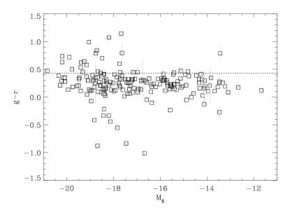
Figure 9.— Color magnitude diagram of the XMPs. The dotted line shows the color threshold to be a blue compact dwarf galaxy according to Gil de Paz et al. (2003). Most XMPs are bluer than this threshold, however, many of them are not dwarfs; often $M_{g}\leq-18$.

4.4. Number density of XMPs in the local Universe

The SDSS spectroscopic legacy sample was designed as a magnitude-limited survey. Therefore, it is relatively simple to correct for the luminosity bias (i.e., the Malmquist bias) and so, to compute the volume density of particular objects. In Paper I  we carried out an estimate of the number density of XMPs in the local Universe. Since the number of XMPs has increased substantially from Paper I, such an estimate has become obsolete, and is updated here.

We employ the so-called $V_{max}$ approximation by Schmidt (1968) used to, e.g., determine luminosity functions of galaxies (Takeuchi et al. 2000). The number density of galaxies with the property $X$, $n(X)$, is just

$$n(X)=\sum_{i}{1\over{V_{i}}},$$ (10)

where the sum includes all galaxies in the sample with property $X$, and $V_{i}$ represents the maximum volume in which the $i$-th galaxy of the sample could be observed. In a magnitude-limited sample, so that all galaxies brighter than the apparent magnitude $m_{lim}$ are included,

$$V_{i}={{d_{i}^{3}}\over{3}}\Omega,$$ (11)

with $\Omega$ the solid angle covered by the survey, and $d_{i}$ the maximum distance at which the $i-$th galaxy can be observed,

$$\log(d_{i}/l_{i})={{1}\over{5}}(m_{lim}-m_{i}).$$ (12)

The maximum distance depends on the absolute magnitude of the galaxy, which can we written in terms of the distance to the galaxy, $l_{i}$, and the apparent magnitude, $m_{i}$, as it has been done for Eq. (12).

A few caveats are in order before applying Eq. (10) to the dataset. SDSS is not truly magnitude limited for a number of reasons. Some bright galaxies are not observed in crowded field due to fiber collision (see Stoughton et al. 2002). Low surface brightness galaxies tend to be missed even if they have significant integrated magnitudes (e.g., Blanton et al. 2005; James et al. 2015). The actual galaxy catalog sample also contain objects coming from complementary SDSS searches, which often are fainter than the magnitude limit of the main survey. The first problem is of no relevance since most observed XMP galaxies are isolated (Filho et al. 2015). The second problem is likely more serious since very faint galaxies tend to have low surface brightness as well (Skillman 1999). Quiescent XMP galaxies like Leo P (Skillman et al. 2013) or KJ 78 (James et al. 2015) show a surface brightness around 24 mag arsec^-2, and objects like them would hardly appear in our selection since SDSS is almost blind at this low surface brightness (Blanton et al. 2005). As it is discussed in the introduction of the paper, we bypass the problem dividing XMPs into quiescent and bursting. Our search in SDSS is sensitive to the bursting XMPs only, and so are the properties derived here. This also holds for the number density to be inferred assuming a magnitude limited sample. The third caveat, namely the existence of XMPs from complementary searches, is also an issue since a significant part of our XMPs belong to these additional catalogs. We solve this problem by applying Eq. (12) only to those XMPs with $m_{i}<m_{lim}$. Using $m_{lim}=17.8$ in the filter $r$, then Eqs. (10), (11), and (12) render

$$n\big{(}{\rm O/H}\leq{1\over{10}}\,{\rm O/H}_{\odot})=(3.4\pm 0.9)\,\times 10^{-3}\,{\rm Mpc^{-3}},$$ (13)

with the error bar considering only the poissonian error associated with the process of galaxy counting.

The density in equation (13) is larger than the density obtained from the sample in Paper I, which is consistent with the fact that the present work contains almost ten times more targets. In terms of the total number of galaxies, XMPs represent some 2 % of all galaxies in a given local volume. The number density of galaxies in the local universe, $\sim 0.17\,{\rm Mpc^{-3}}$, has been taken from the normalization of the total $r$-band luminosity function of SDSS galaxies by Blanton et al. (2005), which includes galaxies brighter than absolute magnitude -12. Even with a significant increase with respect to the previous estimate in Paper I, XMP galaxies are still rare.

4.5. Low-metallicity threshold

One of the puzzling properties of XMP galaxies is the existence of a threshold for the lowest metallicity. This threshold is also present in the XMPs revealed here. Figures 2a and 2b show that

$$12+\log({\rm O/H})\gtrsim 7.1,$$ (14)

which approximately corresponds to 1/40 times the oxygen abundance in the solar composition. This value is similar to, although slightly higher than, the record-breaking low-abundance galaxy SBS0335-052W ($12+\log({\rm O/H})\simeq 7.0$, corresponding to 1/50th of the solar composition; Izotov et al. 2009).

The reason why such a threshold exists is still a riddle. The metallicity of the gas produced during the Big Bang is virtually metal-free, and population III stars contaminate the inter-galactic medium with a metallicity lower than $10^{-4}$ times the solar metallicity (e.g., Bromm & Larson 2004). One can envisage that some of the galaxies formed from this pristine gas have been so dull forming stars that they still retain part of the original gas. Why none of these pristine galaxies is producing stars at present? Several explanations have been offered in the literature, going from the self-enrichment of the HII region used for measuring, to technical difficulties for metallicity determinations below the threshold (see Kunth & Lebouteiller 2011). One additional possibility is offered by the cosmic-web gas-accretion scenario, where the starbursts in XMPs are triggered by gas recently accreted from the cosmic web (see Sánchez Almeida et al. 2014a, and references therein). Numerical simulations predict the cosmic web gas to accumulate metals from the metal-enriched outflows of dwarf galaxies. These metals add up along the Hubble time so that at redshift zero the cosmic-web metallicity is predicted to have a value close to the observed threshold (e.g., Oppenheimer et al. 2012). Should this explanation were correct, then the observational lower limit is tracing the metal content of the cosmic web at present.

4.6. Morphology

Papaderos et al. (2008), Paper I, and later Filho et al. (2013) pointed out that bursting XMPs tend to be cometary or tadpole-like. Such association between metallicity and morphology is notable since metallicity is a property dictated by the spectrum and, therefore, it implies that the spectrum conditions the morphology of the galaxy. In order to check whether the new sample of XMPs maintains this preference for the cometary shape, we repeated the eyeball classification carried out by Filho et al. (2013), which was based on the scheme presented in Paper I. The galaxies may be (1) symmetric if they present a centrally concentrated emission with no obvious structure in the outskirts, (2) cometary for a head-tail structure with an identifiable knot at the head, (3) 2-knot for a structure with two knots, and (4) multi-knot for a diffuse structure with multiple star-formation knots, including irregular galaxies. Figure 10 illustrates these classes with two examples of each galaxy morphology.

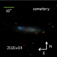
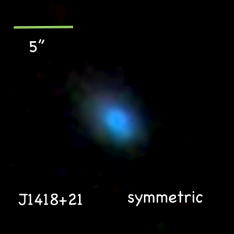
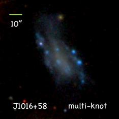
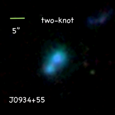
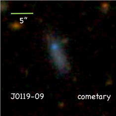
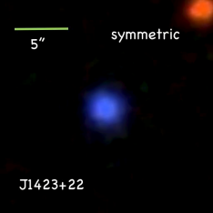
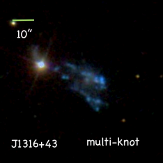
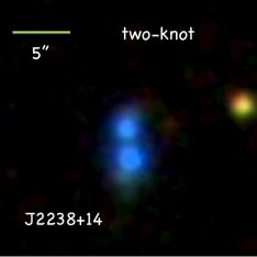
Figure 10.— Examples of the various morphological types found among the XMPs; from left to right cometary, symmetric, multi-knot, and two-knot (see main text for details). The bar on top of each image gives an angular scale on the sky. The image on the top-left panel also points out north and east, which are common to all images. Galaxy images are from SDSS-DR12. The two-knot example on the upper row corresponds to IZw18.

We use color images from SDSS for the visual inspection, and the result of the classification turns out to be,

Cometary 57 %,

Symmetric 23 %,

Multi-knot 10 %,

2-knot 4 %,

others 6 %.

(15)

In agreement with previous estimates, cometary happens to be the dominant shape. Asymmetric shapes (i.e., cometary plus 2-knot plus multi-knot) represent 71 % of the sample. These results are in quantitative agreement with Paper I, where 75% of the targets are asymmetric, and with Filho et al. (2013), where cometary, multi-knot and 2-knot represented 52 % , 16%, and 10% of the XMP sample, respectively. Perhaps the main difference is a slight excess of symmetric targets in the present sample, which we attribute to insufficient spatial resolution since our targets have larger redshifts than the other samples (Sect. 4.3), thus complicating the detection of sub-structure. In addition, this time we include a 5th class to the classification (others in Eq. [15]) to collect objects that do not fit in the main categories easily (e.g., mergers, or elongated galaxies without an identifiable knot). In addition, two of the objects are HII regions in the outskirts of large spirals (# 20 and 59).

We note that a significant part of the symmetric objects looks like the green peas first described by Cardamone et al. (2009). One example is shown in Fig. 10 – the blue symmetric galaxy J1423+22. Depending on the redshift, green-pea like galaxies may look green, pink or blue in SDSS images (Sánchez Almeida et al. 2013a). The identification of green peas with metal-poor galaxies was carried out by Amorín et al. (2010, 2012a), and their rounded morphology seems to be associated with limitations in spatial resolution rather than being intrinsic (e.g., Amorín et al. 2014). The finding of green peas in our sample is encouraging since it naturally connects local XMPs to those expected at higher redshifts, which will appear in surveys deeper than SDSS-DR7 (e.g., eBOSS within SDSS IV).

4.7. Underlying stellar populations

Figure 11.— Mass-weighted stellar age vs light-weighted stellar age for the XMPs, both derived using starlight (Sect. 3.1). The light-weighted mean is biased toward the younger stellar populations, whereas the mass-weighted mean is not. The vertical dashed line shows a light-weighted stellar age of 1 Gyr. Note that most XMPs are to the left of this threshold and thus present a stellar spectrum typical of young stellar populations. The horizontal dashed line shows a mass-weighted stellar age of 1 Gyr. Most XMPs are above this line implying that, despite their seemingly young spectrum, XMPs also contain aged stellar populations – often 10 Gyr old. The ages in the axes are given in Gyr, and the slanted solid line corresponds to the one-to-one relationship.

In order to decontaminate the emission-line fluxes from stellar absorption, we fitted a composite stellar spectrum to the observed continuum (Sect. 3.1). As byproduct of this exercise, we have information on the stellar populations co-existing with the gas responsible for the emission line spectrum. The stellar-population decomposition is not free from uncertainties and degeneracies, however, it suffices to provide a general view of the stellar properties (e.g., Cid Fernandes et al. 2005, 2014).

We find that the underlying stellar populations are generally young, although in almost all cases there are also old stellar components contributing to the observed spectrum. This can be appreciated in Fig. 11, which shows the mass-weighted stellar age versus the light-weighted stellar age for the set of XMPs. The light-weighted mean is strongly biased toward young stars, and we find that most light-weighted ages are younger than 1 Gyr (i.e., they are to the left of the vertical dashed line in Fig. 11). The mass-weighted mean, however, does not suffer from this bias, and most XMPs have mass-weighted ages significantly larger than 1 Gyr (i.e., they are above the horizontal dashed line in Fig. 11). In other words, most XMPs seem to have been forming stars not only at present but also during the last Gyr. On top of this recent star-formation, most of them contain old stars, often as old as 10 Gyr or so. The fact that the class of XMP galaxies contains evolved stellar populations is by no means unknown (see Sect. 1). Their large difference between mass-weighted age and light-weighted age is common to most local star-forming galaxies (e.g., Pérez-Montero et al. 2010; Sánchez Almeida et al. 2012).

4.8. Large scale environment

As it was done by Filho et al. (2015) for the XMPs in Paper I, we have explored the large scale environment of the new list of bursting XMPs using constrained N-body cosmological numerical simulations of the local universe (Nuza et al. 2014a). The cosmological parameters provide a statistical description of the Universe. The constrained simulation that we use selects a particular realization of the current cosmological model that reproduces the spatial distribution of galaxies in the local universe as observed by 2MRS (Huchra et al. 2012). The method is based on a self-consistent Bayesian machine-learning algorithm, and it provides a description of the local cosmic web dark matter with a resolution around 2 Mpc in a box of 180 Mpc$\,h^{-1}$ side (Kitaura et al. 2012; Heß et al. 2013; Kitaura 2013). This simulation, tuned to replicate the local distribution of galaxies, tell us whether the gravitational field at each point forces the matter to collapse in three directions (knot), in two directions (filament), in one direction (sheet), or if the matter is expanding in all three directions (void). This classification, based on the local gravitational potential, correlates very well with the local dark-matter overdensity, which increases from voids to knots. The tendency of a particular type of galaxy to prefer one of the four environments is quantified in terms of the excess probability ratio $\eta(\tau,\epsilon)$, defined as the ratio between the probability that a galaxy of type $\tau$ appears in environment $\epsilon$, and the probability of having any type of galaxy in this environment. The excess probability for the XMPs is shown in Fig. 12. For reference, the figure also includes the excess probability for ellipticals (E), lenticulars (SO), spirals (Sp) and irregulars (Irr) as worked out from 2MRS galaxies by Nuza et al. (2014a). Clearly, XMPs have a strong tendency to appear in voids and to avoid knots. This tendency is more clear in XMPs than in any of the other galaxy types.

Figure 12.— Excess probability ratio for the XMPs. E, S0, Sp, and Irr galaxies are also included for reference (see main text for details). The four panels correspond to the four types of environments: voids, sheets, filaments, and knots. XMPs have a strong tendency to appear in voids and to avoid knots.

These results are very similar to those found by Filho et al. (2015) for the XMPs in Paper I.

5. Discussion and conclusions

Due to their astrophysical interest and rareness (Sect. 1), we have carried out a systematic search for XMP galaxies in SDSS-DR7. Starting from all galaxies with spectra having redshift smaller than 0.25, we end up with a list of only 196 XMPs (Table 1). We select galaxies having [OIII]$\lambda$4363 particularly intense with respect to [OIII]$\lambda$4959 and [OIII]$\lambda$5007. As it is explained in Sect. 2, this implies having a high temperature gas and, since metals are efficient coolants, it is the fingerprint of low-metallicity gas. A first automated search was carried out using k-means to classify all galaxy spectra according to the shape in the region that contains [OIII]$\lambda$4363 and [OIII]$\lambda\lambda$4959,5007. The 1281 objects in the classes of high [OIII]$\lambda$4363 underwent a closer scrutiny by computing their O abundance using the method by Pérez-Montero (2014, Sect. 3.2), which is a model-based approach consistent with the direct method. Those with abundance smaller than one tenth of the solar value ended up in the final list (Table 1). The existence of uncertainty in the metallicity determination, typically 0.17 dex, implies that some of the XMPs are false positives, and some of the discarded targets are false negatives (Appendix A). We offer a second list with 332 XMP candidates (Table 2), selected under less restrictive noise conditions, which contains objects that upon refinement of the metallicity estimate may turn out to be XMPs. The search in the present paper is complementary to the one carried out in Paper I , where k-means is used in the spectral region around H$\alpha$, where the metal-poor signpost is the weakening of [NII]$\lambda$6549 and [NII]$\lambda$6583 with respect to H$\alpha$. From the 196 galaxies in Table 1, only 31 are known as inferred by comparison with the compilation carried out in Paper I, and with the new targets in Izotov et al. (2012). The remaining 165 objects seem to be new members of the XMP class. Among the unknown members, 18 have $12+\log({\rm O/H})\leq 7.50$.

As part of the procedure to measure O/H, we also determine the ratio N/O (Sect. 3.2). Closed-box stellar evolution over long timescales predicts $\log({\rm N/O})$ to be of the order -1.5 at low metallicity, and when $12+\log({\rm O/H})>8$ it increases linearly with increasing metallicity reaching $\simeq-1.0$ at solar metallicity (e.g., Henry & Worthey 1999; Köppen & Hensler 2005). Most XMPs have N/O consistent with the value expected at low metallicity, however, a number of them shows $\log({\rm N/O})\simeq-1.0$ or even larger (Figs. 2a and 7). Metal-poor galaxies with $\log({\rm N/O})\simeq-1.0$ are not very common, but examples do exist in the literature. For instance, the so-called green-pea galaxies have high N/O despite their low metallicity (Amorín et al. 2010, 2012b, ; we have several such green peas among our XMP galaxies – see Sect. 4.6). Moreover, some of the classical XMPs also show enhanced N/O (Morales-Luis et al. 2014). XMPs with large N/O do not appear in Paper I, since we selected galaxies having weak N lines and so our search was biased toward XMPs of low N/O . A simple interpretation for having both large N/O and low O/H is the accretion of significant amounts of metal-poor gas onto galaxies having solar metallicity inter-stellar medium (ISM; e.g., Amorín et al. 2010, and references therein). The mixing of metal-poor gas with pre-existing metal-rich gas drops down the metallicity (i.e., increases H in O/H), but it does not modify the original N/O, which remains as for a metal-rich ISM. Some 10 % of the XMPs have $\log({\rm N/O})\geq-1.2$, representing objects where the accretion of metal-poor gas is arguably part of their star-formation history. Note that accretion will remain unnoticed when the pre-existing ISM presents low N/O. Interpreting N/O as a tracer of previous star-formation episodes is consistent with the trend we observe for the reddening to increase with increasing N/O (Fig. 5b). The correlation naturally arises if part of the dust responsible for extinction was produced together with the N and O in previous star formation episodes.

We quantify the global properties of the XMPs. They have a mean stellar mass around $10^{8}\,{\rm M}_{\odot}$, but with very large scatter going from $10^{6}\,{\rm M}_{\odot}$ to $10^{10}\,{\rm M}_{\odot}$, therefore some of them are fairly massive (Sect. 4.2). We find that both N/O and extinction increase with increasing stellar mass, so that the contribution of evolved stellar populations to the metal content and dust is more important in massive galaxies. From the reddening of the emission line spectrum we infer the dust-mass column density to be around 0.2 ${\rm M_{\odot}\,pc^{-2}}$, which renders a very moderate extinction coefficient (Sect. 4.1). For typical star-forming region size, the dust mass is between 200 and 20,000 ${\rm M}_{\odot}$. We analyze the morphology of the XMPs, finding results in the line of previous studies showing a strong tendency for the XMPs to be tadpole-like or cometary (Papaderos et al. 2008; Paper I; Filho et al. 2013). Explicitly, 71 % are cometary or knotted, and only 23 % of them are symmetric (see Sect. 4.6). As a by-product of the procedure to determine gas phase metallicity, we fit the observed continuum spectrum as a superposition of single stellar populations of varied ages and metallicities. According to such decomposition, the XMPs are characterized by a fairly young stellar spectrum ($<1\,{\rm Gyr}$), although young and aged stellar populations co-exists at the low-metallicity starbursts (Sect. 4.7).

Since the parent sample used to select the XMPs is limited in apparent magnitude, it is relatively simple to estimate the number density of XMPs in the local Universe. We worked it out in Sect. 4.4, finding some $3.4\times 10^{-3}$ XMPs per cubic Mpc (Eq. [13]). This density is significantly larger than the density obtained from the sample in Paper I, and it represents some 2 % of all galaxies in a volume. We also work out the large-scale environment of the XMPs using constrained cosmological numerical simulations (Sect. 4.8). XMPs have a strong tendency to appear in voids and to avoid cluster environments.

One of the most intriguing properties of XMPs is the existence of a lower limit metallicity, of the order of 2 % the solar metallicity. The limit remains in our list (Sect. 4.5), despite the fact that the sample is significantly larger than previous one, and that we have systematically search the full SDSS spectroscopic sample. One of the ways out is, once again, the infall of inter-galactic gas feeding the star-formation process. The inter-galactic gas collects metals ejected from galaxies along the Hubble time, which yields a small but non-zero metallicity expected to be around the value of the observed threshold (Sánchez Almeida et al. 2014a, and references therein).

A caveat to keep in mind is that any search for XMPs based on optical surveys, such as the one we present, overlooks faint low surface brightness galaxies. We are sensitive to star-bursting XMPs (see Sect. 1). As pointed out by, e.g., Skillman et al. (2013; see also Sect. 1), most XMPs may be low surface brightness quiescent XMPs, so that to identify them one would have to resort to blind HI surveys like the Arecibo Legacy Fast ALFA Survey (ALFALFA; Haynes et al. 2011) that led to the discovery of Leo P (Giovanelli et al. 2013).

Appendix A Number of false positives and negatives

For the sake of compactness, we will use the symbol $X_{i}$ to denote the value of 12+log(O/H) in the i-th XMP galaxy. By definition, $X_{i}<X_{0}$, with $X_{0}$ the threshold to be XMP. Bayes’s theorem (e.g., Martin 1971) provides the probability that the true metallicity is $X$ given that we have observed $X_{i}$,

$$P(X|X_{i})=P(X_{i}|X)\,H(X)/P(X_{i}),$$ (A1)

where $P(X_{i}|X)$ stands for the probability of measuring $X_{i}$ when the true metallicity is $X$, $H(X)$ represents the probability the galaxy has a true metallicity $X$, and $P(X_{i})$ corresponds to the probability that the measured metallicity of the galaxy is $X_{i}$ considering all possible values of the true metallicity, i.e.,

$$P(X_{i})=\int_{-\infty}^{\infty}P(X_{i}|X)\,H(X)\,dX.$$ (A2)

If $X$ is larger than the threshold metallicity $X_{0}$, Eq. (A1) provides the probability that the galaxy gives a false positive if its true metallicity is $X$. Since the true metallicity yielding false positives can be any value larger than the threshold, the total probability of a false positive $P(X\geq X_{0}|X_{i})$ is just the sum over all possibilities, i.e., an integral of Eq. (A1) for all $X\geq X_{0}$, namely,

$$P(X\geq X_{0}|X_{i})=\int_{X_{0}}^{\infty}P(X_{i}|X)\,H(X)\,dX\Big{/}\int_{-\infty}^{\infty}P(X_{i}|X)\,H(X)\,dX.$$ (A3)

Assuming the distribution of observational errors to be Gaussian, the probability of measuring $X_{i}$ when the true metallicity is $X$ turns out to be,

$$P(X_{i}|X)=\exp\big{\{}-{{1}\over{2}}[(X_{i}-X)/\sigma_{i}]^{2}\big{\}}/\sqrt{2\pi}\sigma_{i},$$ (A4)

with $\sigma_{i}$ the error, i.e., the square root of the variance of the distribution of errors. Equation (A3) quantifies the probability that a single galaxy gives a false positive, i.e., it gives the number of false positives per galaxy. When we consider the full set, then the total number of false positives $N_{\rm false+}$ is the sum of the number of false positives for all XMP galaxies, i.e.,

$$N_{\rm false+}=\sum_{i}^{\forall\,{\rm XMP}}\,P(X\geq X_{0}|X_{i}).$$ (A5)

By definition, false negatives are true XMPs than end up having $X_{i}>X_{0}$. The number of false negatives, $N_{\rm false-}$, can be worked out in a way similar to the derivation of $N_{\rm false+}$. This time the sum is over all non-XMP galaxies,

$$N_{\rm false-}=\sum_{j}^{\forall\,{\rm non-XMP}}\,P(X<X_{0}|X_{j}),$$ (A6)

with

$$P(X<X_{0}|X_{j})=\int^{X_{0}}_{-\infty}P(X_{j}|X)\,H(X)\,dX\Big{/}\int_{-\infty}^{\infty}P(X_{j}|X)\,H(X)\,dX,$$ (A7)

giving the probability of being XMP even though the measured metallicity $X_{j}$ is larger than the threshold $X_{0}$.

Assuming that the probability density function of possible oxygen abundances $H(X)$ is given by the observed histogram of abundances in Fig. 2b, and using the metallicities and their errors derived in Sect. 3.3, Eqs. (A3), (A4), (A5), (A6), and (A7) yield,

$$N_{\rm false+}\simeq 82,$$ (A8)

$$N_{\rm false-}\simeq 46.$$

If we assume a uniform distribution of abundances in the interval $7\leq 12+\log({\rm O/H})\leq 8.5$, then

$$N_{\rm false+}\simeq N_{\rm false-}\simeq 55.$$ (A9)

References

- Abazajian et al. (2009) Abazajian, K. N., Adelman-McCarthy, J. K., Agüeros, M. A., et al. 2009, ApJS, 182, 543
- Aloisi et al. (2007) Aloisi, A., Clementini, G., Tosi, M., et al. 2007, ApJ, 667, L151
- Amorín et al. (2012a) Amorín, R., Pérez-Montero, E., Vílchez, J. M., & Papaderos, P. 2012a, ApJ, 749, 185
- Amorín et al. (2014) Amorín, R., Sommariva, V., Castellano, M., et al. 2014, A&A, 568, L8
- Amorín et al. (2012b) Amorín, R., Vílchez, J. M., Hägele, G. F., et al. 2012b, ApJ, 754, L22
- Amorín et al. (2010) Amorín, R. O., Pérez-Montero, E., & Vílchez, J. M. 2010, ApJ, 715, L128
- Andrews & Martini (2013) Andrews, B. H. & Martini, P. 2013, ApJ, 765, 140
- Annibali et al. (2013) Annibali, F., Cignoni, M., Tosi, M., et al. 2013, AJ, 146, 144
- Asplund et al. (2009) Asplund, M., Grevesse, N., Sauval, A. J., & Scott, P. 2009, ARA&A, 47, 481
- Baldwin et al. (1981) Baldwin, J. A., Phillips, M. M., & Terlevich, R. 1981, PASP, 93, 5
- Bell & de Jong (2001) Bell, E. F. & de Jong, R. S. 2001, ApJ, 550, 212
- Berg et al. (2012) Berg, D. A., Skillman, E. D., Marble, A. R., et al. 2012, ApJ, 754, 98
- Blanton et al. (2005) Blanton, M. R., Lupton, R. H., Schlegel, D. J., et al. 2005, ApJ, 631, 208
- Brinchmann et al. (2004) Brinchmann, J., Charlot, S., White, S. D. M., et al. 2004, MNRAS, 351, 1151
- Bromm & Larson (2004) Bromm, V. & Larson, R. B. 2004, ARA&A, 42, 79
- Bruzual & Charlot (2003) Bruzual, G. & Charlot, S. 2003, MNRAS, 344, 1000
- Cardamone et al. (2009) Cardamone, C., Schawinski, K., Sarzi, M., et al. 2009, MNRAS, 399, 1191
- Cardelli et al. (1989) Cardelli, J. A., Clayton, G. C., & Mathis, J. S. 1989, ApJ, 345, 245
- Cid Fernandes et al. (2014) Cid Fernandes, R., González Delgado, R. M., García Benito, R., et al. 2014, A&A, 561, A130
- Cid Fernandes et al. (2005) Cid Fernandes, R., Mateus, A., Sodré, L., Stasińska, G., & Gomes, J. M. 2005, MNRAS, 358, 363
- Corbin et al. (2008) Corbin, M. R., Kim, H., Jansen, R. A., Windhorst, R. A., & Cid Fernandes, R. 2008, ApJ, 675, 194
- Dekel et al. (2009) Dekel, A., Birnboim, Y., Engel, G., et al. 2009, Nature, 457, 451
- Doe et al. (2007) Doe, S., Nguyen, D., Stawarz, C., et al. 2007, in Astronomical Society of the Pacific Conference Series, Vol. 376, Astronomical Data Analysis Software and Systems XVI, ed. R. A. Shaw, F. Hill, & D. J. Bell, 543
- Draine (2003) Draine, B. T. 2003, ARA&A, 41, 241
- Ekta & Chengalur (2010) Ekta, B. & Chengalur, J. N. 2010, MNRAS, 406, 1238
- Ferland et al. (2013) Ferland, G. J., Porter, R. L., van Hoof, P. A. M., et al. 2013, Rev. Mexicana Astron. Astrofis., 49, 137
- Filho et al. (2015) Filho, M. E., Sánchez Almeida, J., Muñoz-Tuñón, C., et al. 2015, ApJ, 802, 82
- Filho et al. (2013) Filho, M. E., Winkel, B., Sánchez Almeida, J., et al. 2013, A&A, 558, A18
- Filho (2015b) Filho, M. e. a. 2015b, in preparation
- Fisher et al. (2014) Fisher, D. B., Bolatto, A. D., Herrera-Camus, R., et al. 2014, Nature, 505, 186
- Freeman et al. (2001) Freeman, P., Doe, S., & Siemiginowska, A. 2001, in Society of Photo-Optical Instrumentation Engineers (SPIE) Conference Series, Vol. 4477, Astronomical Data Analysis, ed. J.-L. Starck & F. D. Murtagh, 76–87
- García-Benito & et al. (2015) García-Benito, M. & et al. 2015, in preparation
- Gil de Paz et al. (2003) Gil de Paz, A., Madore, B. F., & Pevunova, O. 2003, ApJS, 147, 29
- Giovanelli et al. (2013) Giovanelli, R., Haynes, M. P., Adams, E. A. K., et al. 2013, AJ, 146, 15
- Guseva et al. (2015) Guseva, N. G., Izotov, Y. I., Fricke, K. J., & Henkel, C. 2015, A&A, 579, A11
- Guseva et al. (2009) Guseva, N. G., Papaderos, P., Meyer, H. T., Izotov, Y. I., & Fricke, K. J. 2009, A&A, 505, 63
- Hägele et al. (2008) Hägele, G. F., Díaz, Á. I., Terlevich, E., et al. 2008, MNRAS, 383, 209
- Haynes et al. (2011) Haynes, M. P., Giovanelli, R., Martin, A. M., et al. 2011, AJ, 142, 170
- Henry & Worthey (1999) Henry, R. B. C. & Worthey, G. 1999, PASP, 111, 919
- Heß et al. (2013) Heß, S., Kitaura, F.-S., & Gottlöber, S. 2013, MNRAS, 435, 2065
- Huchra et al. (2012) Huchra, J. P., Macri, L. M., Masters, K. L., et al. 2012, ApJS, 199, 26
- Izotov et al. (2009) Izotov, Y. I., Guseva, N. G., Fricke, K. J., & Papaderos, P. 2009, A&A, 503, 61
- Izotov et al. (2004) Izotov, Y. I., Stasińska, G., Guseva, N. G., & Thuan, T. X. 2004, A&A, 415, 87
- Izotov et al. (2006) Izotov, Y. I., Stasińska, G., Meynet, G., Guseva, N. G., & Thuan, T. X. 2006, A&A, 448, 955
- Izotov & Thuan (2007) Izotov, Y. I. & Thuan, T. X. 2007, ApJ, 665, 1115
- Izotov et al. (2012) Izotov, Y. I., Thuan, T. X., & Guseva, N. G. 2012, A&A, 546, A122
- James et al. (2015) James, B. L., Koposov, S., Stark, D. P., et al. 2015, MNRAS, 448, 2687
- Kauffmann et al. (2003) Kauffmann, G., Heckman, T. M., Tremonti, C., et al. 2003, MNRAS, 346, 1055
- Kehrig et al. (2015) Kehrig, C., Vílchez, J. M., Pérez-Montero, E., et al. 2015, ApJ, 801, L28
- Kitaura (2013) Kitaura, F.-S. 2013, MNRAS, 429, L84
- Kitaura et al. (2012) Kitaura, F.-S., Erdoǧdu, P., Nuza, S. E., et al. 2012, MNRAS, 427, L35
- Kniazev et al. (2003) Kniazev, A. Y., Grebel, E. K., Hao, L., et al. 2003, ApJ, 593, L73
- Kniazev et al. (2004) Kniazev, A. Y., Pustilnik, S. A., Grebel, E. K., Lee, H., & Pramskij, A. G. 2004, ApJS, 153, 429
- Köppen & Hensler (2005) Köppen, J. & Hensler, G. 2005, A&A, 434, 531
- Krumholz (2013) Krumholz, M. R. 2013, MNRAS, 436, 2747
- Kunth & Lebouteiller (2011) Kunth, D. & Lebouteiller, V. 2011, in EAS Publications Series, Vol. 48, EAS Publications Series, ed. M. Koleva, P. Prugniel, & I. Vauglin, 95–96
- Kunth & Östlin (2000) Kunth, D. & Östlin, G. 2000, A&A Rev., 10, 1
- Lee et al. (2006) Lee, H., Skillman, E. D., Cannon, J. M., et al. 2006, ApJ, 647, 970
- Loveday et al. (2015) Loveday, J., Norberg, P., Baldry, I. K., et al. 2015, MNRAS, 451, 1540
- Ly et al. (2015) Ly, C., Rigby, J. R., Cooper, M., & Yan, R. 2015, ApJ, 805, 45
- Martin (1971) Martin, B. R. 1971, Statistics for Physicists (London: Academic Press Inc)
- Mollá et al. (2009) Mollá, M., García-Vargas, M. L., & Bressan, A. 2009, MNRAS, 398, 451
- Morales-Luis et al. (2014) Morales-Luis, A. B., Pérez-Montero, E., Sánchez Almeida, J., & Muñoz-Tuñón, C. 2014, ApJ, 797, 81
- Morales-Luis et al. (2011a) Morales-Luis, A. B., Sánchez Almeida, J., Aguerri, J. A. L., & Muñoz-Tuñón, C. 2011a, ApJ, 743, 77, Paper I
- Morales-Luis et al. (2011b) Morales-Luis, A. B., Sánchez Almeida, J., Aguerri, J. A. L., & Muñoz-Tuñón, C. 2011b, ApJ, 743, 77
- Nuza et al. (2014a) Nuza, S. E., Kitaura, F.-S., Heß, S., Libeskind, N. I., & Müller, V. 2014a, MNRAS, 445, 988
- Nuza et al. (2014b) Nuza, S. E., Parisi, F., Scannapieco, C., et al. 2014b, MNRAS, 441, 2593
- Oppenheimer et al. (2012) Oppenheimer, B. D., Davé, R., Katz, N., Kollmeier, J. A., & Weinberg, D. H. 2012, MNRAS, 420, 829
- Ordovás-Pascual & Sánchez Almeida (2014) Ordovás-Pascual, I. & Sánchez Almeida, J. 2014, A&A, 565, A53
- Osterbrock (1974) Osterbrock, D. E. 1974, Astrophysics of gaseous nebulae
- Osterbrock (1989) Osterbrock, D. E. 1989, Astrophysics of gaseous nebulae and active galactic nuclei
- Östlin et al. (2001) Östlin, G., Amram, P., Bergvall, N., et al. 2001, A&A, 374, 800
- Pagel et al. (1979) Pagel, B. E. J., Edmunds, M. G., Blackwell, D. E., Chun, M. S., & Smith, G. 1979, MNRAS, 189, 95