Characterizing ground and thermal states of few-body Hamiltonians

Abstract

The question whether a given quantum state is a ground or thermal state of a few-body Hamiltonian can be used to characterize the complexity of the state and is important for possible experimental implementations. We provide methods to characterize the states generated by two- and, more generally, $k$-body Hamiltonians as well as the convex hull of these sets. This leads to new insights into the question which states are uniquely determined by their marginals and to a generalization of the concept of entanglement. Finally, certification methods for quantum simulation can be derived.

Introduction.— Interactions in quantum mechanics are described by Hamilton operators. The study of their properties, such as their symmetries, eigenvalues, and ground states, is central for several fields of physics. Physically relevant Hamiltonians, however, are often restricted to few-body interactions, as the relevant interaction mechanisms are local. But the characterization of generic few-body Hamiltonians is not well explored, since in most cases one starts with a given Hamiltonian and tries to find out its properties.

In quantum information processing, ground and thermal states of local Hamiltonians are of interest for several reasons: First, if a desired state is the ground or thermal state of a sufficiently local Hamiltonian, it might be experimentally prepared by engineering the required interactions and cooling down or letting thermalise the physical system general . For example, one may try to prepare a cluster state, the resource for measurement-based quantum computation, as a ground state of a local Hamiltonian VandenNest2008 . Second, on a more theoretical side, ground states of $k$-body Hamiltonians are completely characterized by their reduced $k$-body density matrices. The question which states are uniquely determined by their marginals has been repeatedly studied and is a variation of the representability problem, which asks whether given marginals can be represented by a global state marginalreview . It has turned out that many pure states have the property to be uniquely determined by a small set of their marginals Linden2002 ; jones , and for practical purposes it is relevant that often entanglement or non-locality can be inferred by considering the marginals only marginalentanglement .

In this paper we present a general approach to characterize ground and thermal states of few-body Hamiltonians. We use the formalism of exponential families, a concept first introduced for classical probability distributions by Amari Amari2001 and extended to the quantum setting in Refs. Hasegawa1997 ; Zhou08 ; Zhou09 ; Niekamp13 . This offers a systematic characterization of the complexity of quantum states in a conceptionally pleasing way. We derive two methods that can be used to compute various distances to thermal states of $k$-body Hamiltonians: The first method is general and uses semidefinite programming, while the second method is especially tailored to cluster and, more generally, graph states. In previous approaches it was only shown that some special states are far away from the eigenstates of local Hamiltonians Haselgrove2003 , but no general method for estimating the distance is known.

Our approach leads to new insights in various directions. First, it has been shown that cluster and graph states can, in general, not be exact ground states of two-body Hamiltonians VandenNest2008 , but it was unclear whether they still can be approximated sufficiently well. Our method shows that this is not the case and allows to bound the distance to ground and thermal states. Second, as shown in Ref. Linden2002 , almost all pure states of three qubits are completely determined by their two-party reduced density matrices. As we prove, for $N\geq 5$ qubits or four qutrits this is not the case, but we present some evidence that the fact might still be true for four qubits. Finally, our method results in witnesses, which can be used in a quantum simulation experiment to certify that a three-body Hamiltonian or a Hamiltonian having long-range interactions was generated.

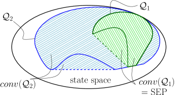
Figure 1: Schematic view of the state space, the exponential families $\mathcal{Q}_{1}$ and $\mathcal{Q}_{2}$, and their convex hulls. While the whole space of mixed states is convex, the exponential families are non-convex low-dimensional manifolds. The convex hull of $\mathcal{Q}_{1}$ are the fully separable states and our approach allows to characterize the convex hull for arbitrary $\mathcal{Q}_{k}$.

The setting.— A two-local (or two-body) Hamiltonian of a system consisting of $N$ spin-1/2 particles can be written as

$$H=\sum\nolimits_{i,j=1}^{N}\sum\nolimits_{\alpha\beta}\lambda_{\alpha\beta}^{(ij)}\sigma_{\alpha}^{(i)}\otimes\sigma_{\beta}^{(j)}\,,$$ (1)

where $\sigma_{\alpha}^{(i)}$ denotes a Pauli matrix $\{\text{1},\sigma_{x},\sigma_{y},\sigma_{z}\}$ acting on the $i$-th particle etc. Note that the identity matrix is included, so $H$ can also contain single particle terms. We denote the set of all possible two-local Hamiltonians by $\mathcal{H}_{2}$ and in an analogous manner the set of $k$-local Hamiltonians by $\mathcal{H}_{k}.$ An example for a two-local Hamiltonian is the Heisenberg model having nearest-neighbor interactions. However, our approach generally ignores any geometrical arrangement of the particles. Finally, for an arbitrary multi-qubit operator $A$ we call the number of qubits where it acts on non-trivially the weight of $A$. In practice, this can be determined by expanding $A$ in terms of tensor products of Pauli operators and looking for the largest non-trivial product.

The set we aim to characterize is the so-called exponential family $\mathcal{Q}_{2}$, consisting of thermal states of two-local Hamiltonians

$$\mathcal{Q}_{2}=\big{\{}\tau\,\big{|}\,\tau=\frac{e^{-\beta H}}{\text{tr}[e^{-\beta H}]}\,,H\in\mathcal{H}_{2}\big{\}}\,.$$ (2)

Ground states can be reached in the limit of infinite inverse temperature $\beta$. For any $k$, the exponential families $\mathcal{Q}_{k}$ can be defined in a similar fashion. The set $\mathcal{Q}_{1}$ consists of mixed product states, the set $\mathcal{Q}_{N}$ of the full state space. The exponential families form the hierarchy $\mathcal{Q}_{1}\subseteq\mathcal{Q}_{2}\subseteq\cdots\subseteq\mathcal{Q}_{N}$, and a suitable $\beta H$ can be seen as a way of parameterizing a specific density matrix $\tau=e^{-\beta H}/\text{tr}[e^{-\beta H}]$. The question arises, what states are in $\mathcal{Q}_{k}$? And for those which are not, what is their best approximation by states in $\mathcal{Q}_{k}$?

It turns out to be fruitful to consider the convex hull

$$\operatorname{conv}(\mathcal{Q}_{2})=\big{\{}\sum\nolimits_{i}p_{i}\,\tau_{i}\,\,|\,\,\tau_{i}\in\mathcal{Q}_{2}\,,\,\sum\nolimits_{i}p_{i}=1\,,\,p_{i}\geq 0\big{\}}\,,$$

and ask whether a state is in this convex hull or not (see also Fig. 1). The convex hull has a clear physical interpretation as it contains all states that can be generated by preparing thermal states of two-body Hamiltonians stochastically with probabilities $p_{i}$. In this way, taking the convex hull can be seen as a natural extension of the concept of entanglement: The thermal states of one-body Hamiltonians are just the mixed product states and their convex hull are the fully separable states of $N$ particles Guehne09 . In this framework, the result of Linden et al. Linden2002 can be rephrased as stating that all three-qubit states are in the closure of the convex hull $\operatorname{conv}(\mathcal{Q}_{2})$, since nearly all pure states are ground states of two-body Hamiltonians.

Finally, the characterization of the convex hull leads to the concept of witnesses that can be used for the experimental detection of correlations Guehne09 . Witnesses are observables which have positive expectation values for states inside a given convex set. Consequently, the observation of a negative expectation value proves that a state is outside of the set. We will see below that such witnesses can be used to certify quantum simulation.

Quantum exponential families.— We recall some results on the characterization of quantum exponential families Zhou09 ; Niekamp13 . Given a state $\varrho$, consider its distance from the exponential family $\mathcal{Q}_{2}$ in terms of the relative entropy (or divergence) $S(\varrho||\tau)=\text{tr}[\varrho(\log(\varrho)-\log(\tau))]$. As the closest state to $\varrho$ in $\mathcal{Q}_{2}$, one obtains the so-called information projection $\tilde{\varrho}_{2}$. It has been shown that the following three characterizations for the information projection $\tilde{\varrho}_{2}\in\mathcal{Q}_{2}$ are equivalent Zhou09 :

(a) $\tilde{\varrho}_{2}$ is the unique minimizer of the relative entropy of $\varrho$ from the set $\mathcal{Q}_{2}$,

$$\tilde{\varrho}_{2}=\operatorname{argmin}_{\tau\in\mathcal{Q}_{2}}S(\varrho||\tau)\,.$$ (3)

(b) Of the set of states having the same two-body reduced density matrices ($2$-RDMs) as $\varrho$, denoted by $\mathcal{M}_{2}(\varrho)$, $\tilde{\varrho}_{2}$ has a maximal von Neumann entropy

$$\tilde{\varrho}_{2}=\operatorname{argmax}_{\mu\in\mathcal{M}_{2}(\varrho)}S(\mu)\,.$$ (4)

(c) Finally, $\tilde{\varrho}_{2}$ is the unique intersection of $\mathcal{Q}_{2}$ and $\mathcal{M}_{2}(\varrho)$. From (b) it follows that if for a state $\sigma$ another state $\varrho$ of higher entropy but having the same $2$-RDMs can be found, then $\sigma$ must lie outside of $\mathcal{Q}_{2}$. A further discussion can be found in Appendix A suppmat .

States not in $\mathcal{Q}_{2}$ are said to have irreducible correlations of order three or higher, because they contain information which is not already present in their $2$-RDMs, if one wishes to reconstruct the global state from its marginals according to Jaynes’ maximum entropy principle Teo2011 . This is conceptionally nice, but also has certain drawbacks. Importantly, the irreducible correlation as quantified by the relative entropy is not continuous, as shown in Ref. Weis2012 . In addition, the relative entropy is difficult to estimate experimentally without doing state reconstruction, so other distances such as the fidelity are preferable. These properties make the relative entropy somewhat problematic and give further reasons why we consider the convex hull.

Characterization via semidefinite programming.— Our first method to estimate the distance of a given state to the convex hull of $\mathcal{Q}_{2}$ relies on semidefinite programming Boyd . This optimization method is insofar useful, as semidefinite programs are efficiently solvable and their solutions can be certified to be optimal. Moreover, ready-to-use packages for their implementation are available.

As a first step we formulate a semidefinite program to test if a given pure $|\psi\rangle$ state is outside of $\mathcal{Q}_{2}$. From the characterization in Eq. (4) it follows that it suffices to find a different state $\varrho$ having the same $2$-RDMs as $|\psi\rangle$. If $\varrho$ is mixed, its entropy is higher than that of $|\psi\rangle$, meaning that $|\psi\rangle$ cannot be its own information projection and therefore lies outside of $\mathcal{Q}_{2}$. If $\varrho$ is pure, consider the convex combination $(|\psi\rangle\langle\psi|+\varrho)/2$, again having a higher entropy. To simplify notation we define for an arbitrary $N$-qubit operator $X$ the operator $R_{k}(X)$ as the projection of $X$ onto those operators, which can be decomposed into terms having at most weight $k$. In practice, $R_{k}(X)$ can be computed by expanding $X$ in Pauli matrices, and removing all terms of weight larger than $k$. Note that $R_{k}(\varrho)$ may have negative eigenvalues.

The following semidefinite program finds a state with the same $k$-body marginals as a given state $|\psi\rangle$:

$$\min_{\varrho}: \quad\text{tr}[\varrho|\psi\rangle\langle\psi|]$$

subject to: $$\quad R_{k}(\varrho)=R_{k}(|\psi\rangle\langle\psi|),$$

$$\quad\text{tr}[\varrho]=1,\quad\varrho=\varrho^{{\dagger}},\quad\varrho\geq\delta\text{1}\,.$$ (5)

While this program can be run with $\delta=0$, it is useful to choose $\delta$ to be strictly positive. Then, a strictly positive $\varrho$ may be found, which is guaranteed to be distant from the state space boundary. Consequently, if $|\psi\rangle$ is disturbed, one can still expect to find a state with the same reduced density matrices in the vicinity of $\varrho$. This can be used to prove that the distance to $\mathcal{Q}_{2}$ is finite, and will allow us to construct witnesses for proving irreducible correlations in $|\psi\rangle$. We make this rigorous in the following Observation. For that, let $\mathcal{B}(|\psi\rangle)$ be the ball in trace distance $D_{\text{tr}}(\mu,\eta)=\frac{1}{2}\text{tr}(|\mu-\eta|)$ centered at $|\psi\rangle$.

Observation 1. Consider a pure state $|\psi\rangle$ and a mixed state $\varrho\geq\delta\text{1}$ with $R_{k}(\varrho)=R_{k}(|\psi\rangle\langle\psi|)$. Then, for any state $\sigma$ in the ball $\mathcal{B}_{\delta}(|\psi\rangle)$ a valid state $\tilde{\varrho}$ in $\mathcal{B}_{\delta}(\varrho)$ can be found, such that their $k$-party reduced density matrices match. Moreover, the entropy of $\tilde{}\varrho$ is larger than or equal to the entropy of $\sigma$. This implies that the ball $\mathcal{B}_{\delta}(|\psi\rangle)$ contains no thermal states of $k$-body Hamiltonians.

The proof is given in Appendix B suppmat .

In the Observation, we considered the trace distance, but a ball in fidelity instead of trace distance can be obtained: Consider a state $\sigma$ near $|\psi\rangle$, having the fidelity $F(\sigma,\psi)=\alpha\geq 1-\delta^{2}$, where $F(\varrho,\psi)=\text{tr}[\varrho|\psi\rangle\langle\psi|]=\langle\psi|\varrho|\psi\rangle$. Then from the Fuchs-van-de-Graaf inequality follows $D_{tr}(\sigma,|\psi\rangle\langle\psi|)\leq\sqrt{1-F(\sigma,{\psi})}\leq\delta\,,$ and Observation 1 is applicable fuchs .

The usage of the fidelity as a distance measure has a clear advantage from the experimental point of view, as it allows the construction of witnesses for multiparticle correlations. Indeed the observable

$$\mathcal{W}=(1-\delta^{2})\text{1}-|\psi\rangle\langle\psi|$$ (6)

has a positive expectation value on all states in $\mathcal{Q}_{k}$ and, due to the linearity of the fidelity, also on all states within the convex hull ${\rm conv}(\mathcal{Q}_{k})$. So, a negative expectation value signals the presence of $k$-body correlations. Witnesses for entanglement have already found widespread applications in experiments Guehne09 .

Equipped with a method to test whether a pure state is in $\operatorname{conv}(\mathcal{Q}_{2})$ or not we are able to tackle the question whether the results of Ref. Linden2002 can be generalized. Recall that in this reference it has been shown that nearly all pure states of three qubits are uniquely determined (among all mixed states) by their reduced two-body density matrices. This means that they are ground states of two-body Hamiltonians. Consequently, the closure of the convex hull $\operatorname{conv}(\mathcal{Q}_{2})$ contains all pure states and therefore also all mixed states, and the semidefinite program in Eq. (5) will not be feasible for $\delta$ strictly positive. The question is whether this result holds for more qubits too.

Concerning pure five-qubit states, we numerically found a fraction of $40\%$ to be outside of $\operatorname{conv}(\mathcal{Q}_{2})$. In the case of pure four-qubit states however, no tested random state has been found to lie outside of $\operatorname{conv}(\mathcal{Q}_{2})$. Given the fact that the test works well in the cases of five and six qubits, this leads us to conjecture that nearly all pure four qubit states are in $\operatorname{conv}(\mathcal{Q}_{2})$, and hence also in $\mathcal{Q}_{2}$. This would imply that a similar result as the one obtained by Ref. Linden2002 holds in the case of four qubits: almost every pure state of four qubits is completely determined by its two-particle reduced density matrix. More details are given in Appendix C suppmat .

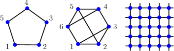
Figure 2: Examples of graphs discussed in this paper. Left: The five-qubit ring-cluster graph. The corresponding ring-cluster state $|C_{5}\rangle$ has a finite distance to the exponential family $\mathcal{Q}_{2}$. Middle: The maximally entangled six-qubit $|M_{6}\rangle$ state is not in the convex hull of $\mathcal{Q}_{3}$. Right: The $2$D periodic $5\times 5$ cluster state $|C_{5\times 5}\rangle$ is not in $\operatorname{conv}(\mathcal{Q}_{4})$.

Characterization via the graph state formalism.— The family of graph states includes cluster states and GHZ states and has turned out to be important for measurement-based quantum computation and quantum error correction hein . Due to their importance, the question whether graph states can be prepared as ground states of two-body Hamiltonians has been discussed before VandenNest2008 . Generally, graph states have shown to not be obtainable as unique non-degenerate ground states of two-local Hamiltonians. Further, any ground state of a $k$-local Hamiltonian $H$ can only be $\epsilon$-close to a graph state $|G\rangle$ with $m(|G\rangle)>k$ at the cost of $H$ having an $\epsilon$-small energy gap relative to the total energy in the system VandenNest2008 . Here $m(|G\rangle)$ is the minimal weight of any element in the stabilizer $S$ of state $|G\rangle$ (see also below). But as pointed out in Ref. VandenNest2008 , this does not imply that graph states cannot be approximated in general, as $\epsilon$ is a relative gap only.

Let us introduce some facts about graph states. A graph consists of vertices and edges (see Fig. 2). This defines the generators

$$g_{a}=\sigma_{x}^{(a)}\prod\nolimits_{b\in N(a)}\sigma_{z}^{(b)},$$ (7)

where the product of the $\sigma_{z}^{(b)}$ runs over all vertices connected to vertex $a$, called neighborhood $N(a)$. The graph state $|G\rangle$ can be defined as the unique eigenstate of all the $g_{a}$, that is $|G\rangle=g_{a}|G\rangle$. This can be rewritten with the help of the stabilizer. The stabilizer $S$ is the commutative group consisting of all possible $2^{N}$ products of $g_{a}$, that is $S=\{s_{i}=\prod_{a\in I}g_{a}\}$. Then, the graph state can be written as $|G\rangle\langle G|=2^{-N}\sum_{s_{i}\in S}s_{i}$ hein . This formula allows to determine the reduced density matrices of graph states easily, since one only has to look at the products of the generators $g_{a}$.

For instance, all stabilizer elements of the five-qubit ring cluster state $|C_{5}\rangle$ have at least weight three, and therefore the $2$-RDMs of $|C_{5}\rangle$ are maximally mixed. By choosing $\delta=2^{-5}$ in Observation $1$, the maximum overlap to $\operatorname{conv}(\mathcal{Q}_{2})$ is bounded by $F_{\tau\in\mathcal{Q}_{2}}(|C_{5}\rangle,\tau)\leq 1-\delta^{2}\approx 0.99902$. Note that Ref. NiekampThesis has demonstrated a slightly better bound $F(|C_{5}\rangle,\tau)\leq 1/32+\sqrt{899/960}\approx 0.99896$. However, both bounds are by far not reachable in current experiments. In fact, one can do significantly better. In the following, we will formulate a stricter bound by first considering $\mathcal{Q}_{2}$ and the ring cluster state $|C_{N}\rangle$ for an arbitrary number of qubits $N\geq 5$, but the result is general.

Observation 2. The maximum overlap between the $N$-qubit ring cluster state $|C_{N}\rangle$ and an $N$-qubit state $\tau\in\mathcal{Q}_{2}$ is bounded by

$$\sup_{\tau\in\mathcal{Q}_{2}}\langle C_{N}|\tau|C_{N}\rangle\leq\frac{D-1}{D}\,,$$ (8)

where $D=2^{N}$ is the dimension of the system. More generally, for an arbitrary pure state with maximally mixed reduced $k$-party states in a $d^{\otimes{N}}$-system, the overlap with $\mathcal{Q}_{k}$ is bounded by $(d^{N}-1)/d^{N}$.

The proof is given in Appendix D suppmat .

In the case of five qubits, $F_{\tau\in\mathcal{Q}_{2}}(|C_{5}\rangle,\tau)\leq 31/32\approx 0.96875$, which improves the bound on the distance to conv$(\mathcal{Q}_{2})$ by more than two orders of magnitude fnx . From Observation 2, we can construct the witness

$$\mathcal{W}=\frac{D-1}{D}\text{1}-|C_{N}\rangle\langle C_{N}|\,,$$ (9)

which detects states outside of $\operatorname{conv}(\mathcal{Q}_{2})$. In a similar fashion, any state having the maximally mixed state as $k$-particle RDMs can be used to construct a witness for $\operatorname{conv}(\mathcal{Q}_{k})$. First, there is a four-qutrit state with maximally mixed 2-RDMs goyeneche , which can be used to derive a witness for $\operatorname{conv}(\mathcal{Q}_{2})$. The highly entangled six-qubit state $|M_{6}\rangle$ (see the graph in Fig. 2) has maximally mixed 3-RDMs, so $\mathcal{W}=\frac{63}{64}\text{1}-|M_{6}\rangle\langle M_{6}|$ is a witness to exclude thermal states of three-body Hamiltonians. Third, consider a $5\times 5$ $2$D cluster state with periodic boundary conditions (see Fig. 2). This state has $m(|C_{5\times 5}\rangle)=5$ VandenNest2008 , and can therefore serve as a witness $\mathcal{W}=\alpha\text{1}-|C_{5\times 5}\rangle\langle C_{5\times 5}|$ for $\operatorname{conv}(\mathcal{Q}_{4})$, where $\alpha=(2^{25}-1)/2^{25}$. It should be noted that this witness can also be used for $\operatorname{conv}(\mathcal{Q}_{2})$, for which the value $\alpha$ might be improved h4note . Finally, the minimal distance $D_{k}$ in terms of the relative entropy from $\mathcal{Q}_{k}$ can be lower bounded by the fidelity distance from its convex hull $\operatorname{conv}(\mathcal{Q}_{k})$, see Appendix D for details suppmat .

Quantum simulation as an application.— The aim of quantum simulation is to simulate a physical system of interest by another well-controllable one. Naturally, it is crucial to ascertain that the interactions really perform as intended. Different proposals have recently come forward to engineer sizeable three-body interactions in systems of cold polar molecules Buechler2007 , trapped ions Bermudez09 , ultracold atoms in triangular lattices Pachos2004 , Rydberg atoms Weimer2010 and circuit QED systems Hafezi2013 . Using the ring cluster state witness $\mathcal{W}=\alpha\text{1}-|C_{N}\rangle\langle C_{N}|$ derived above, it is possible to certify that three- or higher-body interactions have been engineered. This is done by letting the system under control thermalise. If then $\langle\mathcal{W}\rangle<0$ is measured, one has certified that interactions of weight three or higher are present. At least five qubits are generally required for this, but by further restricting the interaction structure, four qubits can be enough for demonstration purposes. This can already be done with a fidelity of $93.75\%$, which is within reach of current technologies. Further details can be found in Appendix E suppmat .

As an outlook, one may try to extend this idea of interaction certification to the unitary time evolution under local Hamiltonians. For instance, digital quantum simulation can efficiently approximate the time evolution of a time-independent local Hamiltonian and in Ref. Lanyon07102011 an effective $6$-particle interaction has been engineered by applying a stroboscopic sequence of universal quantum gates. The process fidelity was quantified using quantum process tomography, however it would be of interest to prove that the same time evolution cannot be generated by $5$-particle interactions only.

Conclusion.— We have provided methods to characterize thermal and ground states of few-body Hamiltonians. Our results can be used to test experimentally whether three-body or higher-order interactions are present. For future work, it would be desirable to characterize the entanglement properties of $\mathcal{Q}_{2}$, e.g. to determine whether the entanglement in these states is bounded, or whether they can be simulated classically in an efficient manner. Furthermore, it is of significant experimental relevance to develop schemes to certify that a unitary time evolution was generated by a $k$-body Hamiltonian.

Acknowledgement.— We thank Tobias Galla, Sönke Niekamp, and Marcin Pawłowski for discussions. This work was supported by the SNSF, the COST Action MP1209, the FQXi Fund (Silicon Valley Community Foundation), the DFG, and the ERC (Consolidator Grant 683107/TempoQ).

I Appendix

I.1 A. Further discussion of the marginal set $\mathcal{M}_{k}(\varrho)$ and its relation to $\mathcal{Q}_{k}$

The marginal set $\mathcal{M}_{k}(\varrho)$ consists of quantum states having the same $k$-party reduced density matrices ($k$-RDMs) as $\varrho$

$$\mathcal{M}_{k}(\varrho)=\{\mu\,|\,\mu_{A}=\varrho_{A}\text{ for all }|A|\leq k\}\,,$$ (10)

where $\mu_{A}$ is the reduced state obtained by tracing out all subsystems not contained in $A$. This set is convex, as its states stay in the marginal family under convex combination.

The exponential family $\mathcal{Q}_{k}$ consists of thermal states of $k$-local Hamiltonians

$$\mathcal{Q}_{2}=\big{\{}\tau\,\big{|}\,\tau=\frac{e^{H}}{\text{tr}[e^{H}]}\,,H\in\mathcal{H}_{2}\big{\}}\,.$$ (11)

In contrast to the marginal set, the exponential families $\mathcal{Q}_{k}$ are, apart from $\mathcal{Q}_{n}$, not convex. To see this, note that $\operatorname{conv}(\mathcal{Q}_{1})$ is the set of separable states, having a volume and a number of free parameters corresponding to the dimension of the state space. In addition, $\operatorname{conv}(\mathcal{Q}_{k})$ is larger than the set of separable states for $k\geq 2$. However, $\mathcal{Q}_{k}$ has not as many free parameters and is a set of measure zero. Thus $\mathcal{Q}_{k}\subsetneq\operatorname{conv}(\mathcal{Q}_{k})$, and $\mathcal{Q}_{k}$ cannot be convex.

The relations between the marginal set and the exponential family originates in two special ways to parametrize a quantum state Hasegawa1997 . These are the affine (also called mixed) and the exponential representations

$$\varrho_{\text{aff}} =\text{1}/D+\eta_{i}A_{i}\,, \eta \in(-1,1)^{D^{2}-1}\,,$$

$$\varrho_{\exp} =\exp[\theta_{i}A_{i}-\psi(\theta)]\,, \theta \in\text{R}^{D^{2}-1}\,,$$ (12)

where $D$ is the dimension of the system, $\{A_{i}\}$ is a suitable orthonormal basis of the operator space, and we sum over repeated indices. The Massieu function $\psi(\theta)=\log\text{tr}[\exp H]$ is not only required for normalization, but also defines, together with the potential $\phi(\eta)=-S(\eta)=\text{tr}[\varrho\log\varrho]$, a Legendre transform $\psi(\theta)+\phi(\eta)-\theta_{i}\eta_{i}=0\,.$ The relations

$$\eta^{i}=\frac{\partial\psi(\theta)}{\partial\theta_{i}}=\text{tr}[\varrho A_{i}]\,,\quad\theta_{i}=\frac{\partial\phi(\eta)}{\partial\eta_{i}}=\text{tr}[HA_{i}]\,,$$ (13)

follow. For any two states $\varrho(\eta)$ and $\varrho^{\prime}(\theta^{\prime})$, the following Pythagorean relation for the relative entropy holds

$$S(\varrho||\varrho^{\prime})=\phi(\eta)+\psi(\theta^{\prime})-\eta_{i}\theta^{\prime}_{i}\,,$$ (14)

and its repeated application yields

$$S(\varrho||\varrho^{\prime\prime})$$

$$=S(\varrho||\varrho^{\prime})+S(\varrho^{\prime}||\varrho^{\prime\prime})+(\eta_{i}-\eta^{\prime}_{i})\cdot(\theta^{\prime}_{i}-\theta^{\prime\prime}_{i})\,.$$ (15)

The information projection $\tilde{\varrho}_{k}$ of $\varrho$ is the element in $\mathcal{M}_{k}(\varrho)$ having the largest von Neumann entropy. Given $\varrho$, its information projection $\tilde{\varrho}_{k}$, and a $\tau\in\mathcal{Q}_{k}$, the Pythagorean relation then simplifies to

$$S(\varrho||\tau)=S(\varrho||\tilde{\rho}_{k})+S(\tilde{\varrho}_{k}||\tau)\,.$$ (16)

The above definition of the information projection is equivalent to $\tilde{\varrho}$ being in the unique intersection of the exponential family $\mathcal{Q}_{k}$ with $\mathcal{M}_{k}(\varrho)$, and to $\tilde{\varrho}_{k}=\operatorname{argmin}_{\tau\in\mathcal{Q}_{k}}S(\rho||\tau)$. This is illustrated in Fig. 3.

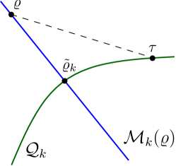
Figure 3: The information projection $\tilde{\varrho}_{k}$ lies in the unique intersection of $\mathcal{Q}_{k}$ and $\mathcal{M}_{k}(\varrho)$. It is also the minimizer of the relative entropy $S(\rho||\cdot)$ in $\mathcal{Q}_{k}$.

We provide two examples. First, consider the five-qubit ring cluster state $|C_{5}\rangle$ and its information projection onto $\mathcal{Q}_{2}$. The state $|C_{5}\rangle$ has maximally mixed $2$-body marginals, and of the set $\mathcal{M}_{2}(|C_{5}\rangle)$, the maximally mixed state has the highest entropy. Second, consider the one-parameter family of states $|GHZ_{\alpha}\rangle=(|000\rangle+e^{i\alpha}|111\rangle)/\sqrt{2}$. All of its two-party reduced states are equal to $(|00\rangle\langle 00|+|11\rangle\langle 11|)/2$. Also,

$$\gamma =\int_{\alpha}\!|GHZ_{\alpha}\rangle\langle GHZ_{\alpha}|\,\mathrm{d}\alpha$$

$$=(|000\rangle\langle 000|+|111\rangle\langle 111|)/2$$ (17)

has the same $2$-RDMs and is thus an element of the marginal set $\mathcal{M}_{2}(|GHZ_{\alpha}\rangle)$. Additionally, $\gamma$ is the information projection of $|GHZ_{\alpha}\rangle$ onto $\mathcal{Q}_{2}$, as it is the element of maximum entropy in $\mathcal{M}_{2}(|GHZ_{\alpha}\rangle)$. As known from Ref. Linden2002 , almost all three qubit states are determined by their 2-RDMs, and thus the irreducible three-body correlation is discontinuous at $|GHZ_{\alpha}\rangle$. More examples can be found in Ref. Niekamp13 .

As a last part in this section, we relate the exponential family $\operatorname{conv}(\mathcal{Q}_{k})$ to the sets of ground and excited states of local Hamiltonians respectively. As argued above, nondegenerate ground states of k-local Hamiltonians $H_{k}\in\mathcal{H}_{k}$ are determined by their k-RDMs and belong to the closure of $\mathcal{Q}_{k}$. Nondegenerate excited states of $k$-local Hamiltonians are completely determined by their $2k$-RMDs Chen2012 , and are therefore ground states of suitable $2k$-local Hamiltonians $H_{2k}\in\mathcal{H}_{2k}$. The argument rests on the fact that any eigenstate of a Hamiltonian $H_{k}$ will also be the ground state of $(H_{k}-\lambda\text{1})^{2}$, where $\lambda$ is the corresponding eigenvalue. A similar argument also holds for nondegenerate ground and eigenstates. But as can be seen by parameter counting, there exist $2k$-local Hamiltonians which cannot be written as $H_{2k}=(H_{k}-\lambda\text{1})^{2}$ with $H_{k}\in\mathcal{H}_{k}$. Thus the set of eigenstates of $k$-local Hamiltonians $\operatorname{ES}(\mathcal{H}_{k})$ is a proper subset of the set of ground states of $2k$-local Hamiltonians $\operatorname{GS}(\mathcal{H}_{2k})$, $\operatorname{ES}(\mathcal{H}_{k})\subsetneq\operatorname{GS}(\mathcal{H}_{2k})$. Finally, thermal states of $k$-local Hamiltonians are in the convex hull of $\operatorname{ES}(\mathcal{H}_{k})$, and it follows that $\operatorname{conv}(\mathcal{Q}_{k})\subsetneq\operatorname{conv}(\operatorname{GS}(\mathcal{H}_{2k}))$.

I.2 B. Proof of Observation 1

Observation 1. Consider a pure state $|\psi\rangle$ and a mixed state $\varrho\geq\delta\text{1}$ with $R_{k}(\varrho)=R_{k}(|\psi\rangle\langle\psi|)$. Then for any state $\sigma$ in the ball $\mathcal{B}_{\delta}(|\psi\rangle)$ a valid state $\tilde{\varrho}$ in $\mathcal{B}_{\delta}(\varrho)$ can be found, such that their $k$-party reduced density matrices match. Moreover, the entropy of $\tilde{}\varrho$ is larger than or equal to the entropy of $\sigma$. This implies that the ball $\mathcal{B}_{\delta}(|\psi\rangle)$ contains no thermal states of $k$-body Hamiltonians.

Proof.

Any $\sigma$ in the trace ball $\mathcal{B}_{\delta}(|\psi\rangle)$ can be written as $\sigma=|\psi\rangle\langle\psi|+X$, with a traceless $X$. The trace can be decomposed as $\text{tr}(X)=\langle\psi|X|\psi\rangle+\sum_{i}\langle\psi_{i}^{\perp}|X|\psi_{i}^{\perp}\rangle=0\,,$ where the $|\psi_{i}^{\perp}\rangle$ are orthogonal to $|\psi\rangle.$ The second term of this expression is positive, since

$$\sum_{i}\langle\psi_{i}^{\perp}|X|\psi_{i}^{\perp}\rangle =\sum_{i}\langle\psi_{i}^{\perp}|(X+|\psi\rangle\langle\psi|)|\psi_{i}^{\perp}\rangle$$

$$=\sum_{i}\langle\psi_{i}^{\perp}|\sigma|\psi_{i}^{\perp}\rangle\geq 0\,.$$ (18)

So we must have $\langle\psi|X|\psi\rangle\leq 0$. Furthermore, $X$ can only have one negative eigenvalue $\lambda_{-}$, otherwise there would be also $|\psi_{i}^{\perp}\rangle$ with $\langle\psi_{i}^{\perp}|X|\psi_{i}^{\perp}\rangle<0$, which is in contradiction to $\sigma\geq 0.$ From $\text{tr}(X)=0$ it follows that $\lambda_{-}$ has the largest modulus of all eigenvalues and consequently $\text{tr}(|X|)=2|\lambda_{-}|$. Since $D_{\text{tr}}(|\psi\rangle\langle\psi|,\sigma)=\text{tr}|X|/2\leq\delta,$ it follows that $|\lambda_{-}|\leq\delta$.

For $\sigma\in\mathcal{B}_{\delta}(|\psi\rangle)$ we choose $\tilde{\varrho}=\varrho+X$ as a candidate having the $k$-RDMs of $\sigma$. We have

$$R_{k}(\sigma)=R_{k}(|\psi\rangle\langle\psi|+X)=R_{k}(\varrho+X)=R_{k}(\tilde{\varrho})\,.$$ (19)

Furthermore, $\tilde{\varrho}$ is a positive semidefinite density matrix, because of $\tilde{\varrho}=\varrho+X\geq(\delta-|\lambda_{-}|)\text{1}\geq 0$. Thus, for any state $\sigma$ in $\mathcal{B}_{\delta}(|\psi\rangle)$ there exists a state $\tilde{\varrho}$ in $\mathcal{B}_{\delta}(\varrho)$, such that the $k$-RDMs of $\sigma$ and $\tilde{\varrho}$ match.

Figure 4: Illustration of Observation 1: If a strictly positive $\varrho$ can be found, then for a given perturbation $\sigma$ of $|\psi\rangle$ one can find a corresponding $\tilde{}\varrho$ in the vicinity of $\varrho$, such that the reduced density matrices of $\sigma$ and $\tilde{}\varrho$ are the same.

Now we show that the entropy of $\tilde{\varrho}$ is larger than or equal to the entropy of $\sigma$, as this ensures that $\sigma$ is not in $\mathcal{Q}_{k}$. Namely, if the entropy of $\tilde{\varrho}$ is larger, a state with the same $k$-RDMs but of higher entropy than $\sigma$ has been found, and $\sigma$ is outside of $\mathcal{Q}_{k}$. If on the other hand equality holds, then again $\sigma\notin\mathcal{Q}_{k}$ due to the uniqueness of the information projection and because of $\sigma\neq\tilde{\varrho}$.

First, note that if $\rho$ fulfills the condition $S(\varrho)\geq 2C_{\delta}$, where $C_{\delta}=-\delta\log(\tfrac{\delta}{D-1})-(1-\delta)\log(1-\delta)$, then also as required $S(\tilde{\varrho})\geq S(\sigma)$. This follows from the sharp Fannes-Audenaert inequality Audenaert2007

$$|S(\eta)-S(\mu)|\leq-d\log\big{(}\frac{d}{D-1}\big{)}-(1-d)\log(1-d)\,,$$ (20)

where $d=D_{\text{tr}}(\eta,\mu)$ and $D=2^{N}$ is the dimension of the system. Recall that $\sigma\in\mathcal{B}_{\delta}(\psi)$ and $\tilde{\varrho}\in\mathcal{B}_{\delta}(\varrho)$. Thus the entropy of $\sigma$ can be at most $C_{\delta}$, and the entropy of $\tilde{\varrho}$ must be at least $S(\varrho)-C_{\delta}$. Requiring $S(\varrho)\geq 2C_{\delta}$ therefore ensures that the entropy of $\tilde{\varrho}$ is higher than or equal to that of $\sigma$.

It remains to show that $\varrho$ indeed fulfills this condition. For that, note that the eigenvalues of $\varrho$ are larger than $\delta$ but smaller than $1/N$ due to the normalization of $\varrho$. Furthermore assume $D\geq 8$, since we are considering at least three qubits. From the bounds on the eigenvalues it follows that the entropy of $\varrho$ is bounded by

$$S(\varrho) \geq-[1-(D-1)\delta]\log[1-(D-1)\delta]$$

$$-(D-1)\delta\log(\delta)\equiv\Gamma\,.$$ (21)

So, we consider the function $\mathcal{F}(\delta,D)=\Gamma-2C_{\delta}$ and have to show its positivity. Let us first fix $D$. Taking the second derivative of $\mathcal{F}$ with respect to $\delta$ one directly finds that this second derivative is strictly negative. This implies that $\mathcal{F}$ assumes only one maximum in the interval $[0,1/D]$ and that the minima are assumed at the borders. We have $\mathcal{F}(0,D)=0$ and it remains to prove that $\mathcal{G}(D)=\mathcal{F}(1/D,D)$ is positive. For $D=8$ one can directly check that $\mathcal{G}$ as well as its derivative is positive. Furthermore, the second derivative of $\mathcal{G}(D)$ with respect to $D$ is strictly positive for any $D\geq 8$, which proves the claim. ∎

I.3 C. Numerical results

Let us first consider states of five and six qubits. We report in Table 1 numerical results for the fraction of pure states lying outside of $\operatorname{conv}(\mathcal{Q}_{2})$, with the condition of positive definiteness $\delta$ ranging from $10^{-3}$ to $10^{-7}$. We tested $300^{\prime}000$ ($30^{\prime}000$) random five-qubit (six-qubit) states distributed to the Haar measure Mezzadri07 with our semidefinite program using the solver MOSEK num:sdp . As can be seen from the Table, at least $40\%$ of all tested five-qubit states and $100\%$ of all tested six-qubit states lie outside of $\operatorname{conv}(\mathcal{Q}_{2})$. Thus, a similar result as in Ref. Linden2002 does not hold in the cases of five and six qubits.

Concerning $\operatorname{conv}(\mathcal{Q}_{3})$, a single five-qubit state and no six-qubit state has been detected to lie outside. We ascribe the latter result to a rather weak statistics, as states in the vicinity of $|M_{6}\rangle$ are easily detected by our semi-definite program (cf. Fig. 2).

Let us now turn to the case of four qubits. Here, none of $8$ million random pure states have been found to be outside of $\operatorname{conv}(\mathcal{Q}_{2})$. The numerical result suggests that this is a general feature of four-qubit systems. We also tested special examples of highly entangled four-qubit states, such as the cluster state, classes of hypergraph states Otfried , the Higuchi-Sudbery $|M_{4}\rangle$ state Higuchi or the $|\chi\rangle$-state Guehne09 ; Osterloh . While many of theses states can be shown to be outside of $\mathcal{Q}_{2}$, we were not able to prove analytically or with the help of the semidefinite program that they have a finite distance to $\mathcal{Q}_{2}$. This implies that they might be approximated by thermal states of two-body Hamiltonians.

$\delta$	$10^{-3}$	$10^{-4}$	$10^{-5}$	$10^{-6}$	$10^{-7}$
$5$qb	0.0040	0.1325	0.2976	0.3729	0.4000
$6$qb	0.7680	0.8872	0.8897	1.0000	1.0000

Table 1: Fraction of pure five and six qubit states which are outside of the convex hulls of $\mathcal{Q}_{2}$, as detected by the semidefinite program from Eq. (5). See the text for further details.

I.4 D. Proof of Observation 2

Observation 2. The maximum overlap between the $N$-qubit ring cluster state $|C_{N}\rangle$ and an $N$-qubit state $\tau\in\mathcal{Q}_{2}$ is bounded by

$$\sup_{\tau\in\mathcal{Q}_{2}}\langle C_{N}|\tau|C_{N}\rangle=\sup_{H\in\mathcal{H}_{2}}\text{tr}\big{[}\frac{e^{H}}{\text{tr}[e^{H}]}|C_{N}\rangle\langle C_{N}|\big{]}\leq\frac{D-1}{D},$$ (22)

where $D=2^{N}$ is the dimension of the system. More generally, for an arbitrary pure state with maximally mixed reduced $k$-party states in a $d^{\otimes{N}}$-system, the overlap with $\mathcal{Q}_{k}$ is bounded by $(d^{N}-1)/d^{N}$.

Proof.

We consider first only the ring cluster state, the generalization is then straightforward. For $N\geq 5$, the ring cluster state $|C_{N}\rangle$ has $m(|C_{N}\rangle)=3$, that is, all the two-body reduced density matrices are maximally mixed VandenNest2008 . Since the family of thermal states is invariant under the addition of the identity $\tau(H)\mapsto\tau(H+\theta\text{1})$, we can choose $H$ to be traceless when maximizing the overlap. So $\text{tr}[H]=0$ and $\text{tr}[H|C_{N}\rangle\langle C_{N}|]=0$ follows. Note that this was the only part in the proof where the property of $|C_{N}\rangle$ having maximally mixed 2-RDMs was required.

We write $H$ and $|C_{N}\rangle\langle C_{N}|$ in the eigenbasis $\{|\eta_{i}\rangle\}$ of $H$,

$$H =\sum_{i}\eta_{i}|\eta_{i}\rangle\langle\eta_{i}|$$

$$|C_{N}\rangle\langle C_{N}| =\sum_{ij}c_{i}c_{j}|\eta_{i}\rangle\langle\eta_{j}|\,,$$ (23)

and obtain following conditions, where the second results from the normalization of the ring cluster state:

$$f_{1} =\sum_{i}\eta_{i}=0\,,$$ (24)

$$f_{2} =\sum_{i}p_{i}-1=0\,, p_{i}=|c_{i}|^{2}\geq 0\,,$$ (25)

$$f_{3} =\sum_{i}p_{i}\eta_{i}=0\,.$$ (26)

Under these conditions, we have to maximize

$$\mathcal{F}=\frac{\sum_{i}p_{i}e^{\eta_{i}}}{\sum_{i}e^{\eta_{i}}}.$$ (27)

If $H$ is nontrivial, it must have both some positive and negative eigenvalues. Then at least two of the $p_{i}$ must be nonzero. We use the method of Lagrange multipliers and consider

$$\Lambda=\frac{\sum_{i}p_{i}e^{\eta_{i}}}{\sum_{i}e^{\eta_{i}}}+\lambda_{1}f_{1}+\lambda_{2}f_{2}+\lambda_{3}f_{3}\,.$$ (28)

If the maximum is attained for some value $p_{k}$ which is not at the border of the domain $[0,1]$, we then must have

$$\frac{\partial\Lambda}{\partial p_{k}}=\frac{e^{\eta_{k}}}{\sum_{i}e^{\eta_{i}}}+\lambda_{2}+\lambda_{3}\eta_{k}=0\,.$$ (29)

For a given spectrum of $H$, $\{\eta\}=(\eta_{1},\dots,\eta_{D})$, Eq. (29) has a solution for at most two values, $\eta_{+}$ and $\eta_{-}$. For any $\eta_{i}$ not equal to $\eta_{+}$ or $\eta_{-}$, the corresponding variable $p_{i}$ has to lie at the boundary of the domain $[0,1]$, which implies that $p_{i}=0$ if $\eta_{i}\notin\{\eta_{+},\eta_{-}\}$. The eigenvalues $\eta_{+}$ and $\eta_{-}$ can be $l$ and $l^{\prime}$ fold degenerate, with corresponding $p_{+}^{l},p_{-}^{l^{\prime}}$. But then, it is easy to see that it is optimal to maximize one of those by taking $p_{+}=\sum_{l}p_{+}^{l}$ and $p_{-}=\sum_{l^{\prime}}p_{-}^{l^{\prime}}$ and setting the others to zero. Second, considering the set of $\eta_{i}\notin\{\eta_{+},\eta_{-}\}$ where $p_{i}=0$ one can further see with Jensen’s inequality that it is optimal to take all of the $\eta_{i}$ equal, that is $(D-2)\eta_{i}=-(\eta_{+}+\eta_{-})$. So, the whole problem reduces to a problem with four variables,

$$\max_{p_{i},\eta_{i}}\mathcal{F}=\max_{p_{\pm},\eta_{\pm}}\frac{p_{+}e^{\eta_{+}}+p_{-}e^{\eta_{-}}}{e^{\eta_{+}}+e^{\eta_{-}}+(D-2)e^{-(\eta_{+}+\eta_{-})/(D-2)}}\,.$$ (30)

From the conditions it follows that we can choose $\eta_{+}>0$, which implies that $\eta_{-}=-\eta_{+}p_{+}/p_{-}<0$. We have to prove that the upper bound is is $(D-1)/D$. Rewriting $p_{-}=\frac{\eta_{+}}{\eta_{+}-\eta_{-}}$, we aim to show that

$$\frac{\left(1-\frac{\eta_{+}}{\eta_{+}-\eta_{-}}\right)e^{\eta_{+}}+\frac{\eta_{+}}{\eta_{+}-\eta_{-}}e^{\eta_{-}}}{e^{\eta_{+}}+e^{\eta_{-}}+(D-2)e^{-(\eta_{+}+\eta_{-})/(D-2)}}\leq\frac{D-1}{D}\,.$$ (31)

This can be rewritten to

$$(D-1)(\eta_{+}-\eta_{-})\big{[}e^{\eta_{+}}+e^{\eta_{-}}+(D-2)e^{-(\eta_{+}+\eta_{-})/(D-2)}\big{]}$$

$$-D(\eta_{+}e^{\eta_{-}}-\eta_{-}e^{\eta_{+}})\geq 0\,.$$ (32)

Regrouping terms leads to

$$\underbrace{(D-1)(D-2)(\eta_{+}-\eta_{-})\exp\left(-\frac{\eta_{+}+\eta_{-}}{D-2}\right)}_{t_{1}}$$

$$\underbrace{-\left[\eta_{+}+(D-1)\eta_{-}\right]\exp(\eta_{-})}_{t_{2}}$$

$$\underbrace{+\left[\eta_{-}+(D-1)\eta_{+}\right]\exp(\eta_{+})}_{t_{3}}\geq 0\,.$$ (33)

The term $t_{1}$ is always positive, while the signs of $t_{2}$ and $t_{3}$ depend upon the choice of $\eta_{+}$ and $\eta_{-}$. So consider the following three cases:

1. Case: $(D-1)\eta_{+}<|\eta_{-}|$: Then $t_{2}\geq 0$, but $t_{3}<0$. However, we have $t_{1}+t_{3}\geq 0$ because of

   $$-(\eta_{+}+\eta_{-})=-\eta_{+}+|\eta_{-}|\geq(D-2)\eta_{+}$$ (34)

   and

   $$(D-1) (D-2)(\eta_{+}-\eta_{-})$$

   $$\geq\, (D-1)(D-2)|\eta_{-}|\geq 2|\eta_{-}|$$

   $$\geq\, |\eta_{-}|+(D-1)\eta_{+}\geq|\eta_{-}+(D-1)\eta_{+}|\,.$$ (35)

2. Case: $(D-1)^{-1}\eta_{+}\leq|\eta_{-}|\leq(D-1)\eta_{+}$: This case directly leads to $t_{2}\geq 0$ and $t_{3}\geq 0$.

3. Case: $|\eta_{-}|<(D-1)^{-1}\eta_{+}$: Then $t_{3}\geq 0$, but $t_{2}<0$. However, we have $t_{2}+t_{3}\geq 0$, because of $e^{\eta_{+}}>e^{\eta_{-}}$ and

   $$(D-1)\eta_{+}+\eta_{-}\geq 3\eta_{+}+\eta_{-}$$

   $$\geq\, 2\eta_{+}\geq\eta_{+}+(D-1)\eta_{-}\,.$$ (36)

This finishes the proof. ∎

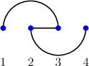
Figure 5: Graph of the linear cluster state $\eta$ with particles $2$ and $3$ exchanged. This state cannot be approximated by Hamiltonians with nearest-neighbor interactions only.

Note that the minimal fidelity distance fidelity distance from the convex hull $\operatorname{conv}(\mathcal{Q}_{k})$ can be used to show the presence of irreducible correlations. The minimal distance $D_{k}$ to $\mathcal{Q}_{k}$ in terms of the relative entropy is bounded by

$$D_{k}(\varrho)\geq\min_{\sigma\in\operatorname{conv}(\mathcal{Q}_{2})}S(\varrho||\sigma)\geq-\log\max_{\sigma\in\mathcal{Q}_{2}}F(\varrho,\sigma)\,.$$ (37)

This follows from a recent result on $\alpha$-Rényi relative entropies Tomamichel2013 ,

$$S(\varrho||\sigma)\geq S_{1/2}(\varrho||\sigma)=-\log F(\varrho,\sigma)\,.$$ (38)

Therefore, the divergence of the five qubit ring cluster state from $\mathcal{Q}_{2}$ is bounded by $D_{2}(|C_{5}\rangle)\geq 0.0317$.

I.5 E. Interaction certification

To certify that higher than two-body interactions have been engineered, a four qubit state can be used by further restricting the possible interaction structure of the system. As an example, consider an ion chain of four qubits in a linear trap, where the only two-body interactions allowed are of the nearest-neighbor type. Then the four-qubit linear cluster state $\eta$, which is a usual linear cluster state with a permutation of particles $2$ and $3$ (see Fig. 5), cannot be obtained as a ground or thermal state but only be approximated up to a fidelity of $\alpha=(N-1)/N=15/16=93.75\%$. This value is within reach of current technologies.

To see why this state cannot be obtained, note that it has the generator $G=\{XIZI,IXZZ,ZZXI,IZIX\}$, where $X,Y,Z,I$ stand for the Pauli matrices and the identity respectively. The stabilizer is then given by

$$S=\{ IIII,IXZZ,IYZY,IZIX,$$

$$XIZI,XXIZ,XYIY,XZZX,$$

$$YIYX,YXXY,-YYXZ,YZYI,$$

$$ZIXX,-ZXYY,ZYYZ,ZZXI\}\,.$$ (39)

The nearest-neighbor marginals of the graph state

$$\eta=2^{-4}\sum_{s_{i}\in S}s_{i}\,,$$ (40)

which are $\eta_{12},\eta_{23}$, and $\eta_{34}$, are all maximally mixed. The remaining two-party marginals do not need to be considered, as long-range interactions are precluded by the physical setup. Then an argument similar to as in Observation $2$ can be made. It is again interesting to see what fraction of states cannot be ground states in such a setup. Our semidefinite program shows that $94\%$ of pure states cannot be approximated as ground or thermal states of a linear spin chain having nearest-neighbor interactions only qsremark2 . However, when including next-to-nearest neighbor interactions, no unobtainable states were detected.

References

- (1) S. Diehl, A. Micheli, A. Kantian, B. Kraus, H.P. Büchler, and P. Zoller, Nat. Phys. 4, 878 (2008); B. Röthlisberger, J. Lehmann, D. S. Saraga, P. Traber, and D. Loss, Phys. Rev. Lett. 100, 100502 (2008); R. Oliveira and B.M. Terhal, Quantum Inform. Comput. 8, 900 (2008); F. Verstraete, M.M. Wolf, and J.I. Cirac, Nat. Phys. 5, 633 (2009); P. Facchi, G. Florio, S. Pascazio, and F. V. Pepe, Phys. Rev. Lett. 107, 260502 (2011); J. Chen, Z. Ji, Z. Wei, and B. Zeng, Phys. Rev. A 85, 040303(R) (2012); F. Ticozzi, L. Viola, Phil. Trans. R. Soc. A 370 5259 (2012).
- (2) M. Van den Nest, K. Luttmer, W. Dür, and H. J. Briegel, Phys. Rev. A 77, 012301 (2008).
- (3) A. J. Coleman, Rev. Mod. Phys. 35, 668 (1963).
- (4) N. Linden, S. Popescu and W. K. Wootters, Phys. Rev. Lett. 89, 207901 (2002).
- (5) N. S. Jones and N. Linden, Phys. Rev. A 71, 012324 (2005); L. Diósi, Phys. Rev. A 70, 010302(R) (2004).
- (6) G. Tóth, Phys. Rev. A 71, 010301(R) (2005); J. Tura, R. Augusiak, A. B. Sainz, T. Vértesi, M. Lewenstein, and A. Acín, Science 344, 1256 (2014); L. Chen, O. Gittsovich, K. Modi and M. Piani, Phys. Rev. A 90, 042314 (2014); N. Miklin, T. Moroder, and O. Gühne, Phys. Rev. A 93, 020104(R) (2016).
- (7) S.-I. Amari, IEEE Trans. Inf. Theory 47, 1701 (2001).
- (8) H. Hasegawa, Rep. Math. Phys. 39, 49 (1997).
- (9) D. L. Zhou, Phys. Rev. Lett. 101, 180505 (2008).
- (10) D. L. Zhou, Phys. Rev. A 80, 022113 (2009).
- (11) S. Niekamp, T. Galla, M. Kleinmann, and O. Gühne, J. Phys. A: Math. Theor. 46, 125301 (2013).
- (12) H. L. Haselgrove, M. A. Nielsen, and T. J. Osborne, Phys. Rev. Lett. 91, 210401 (2003).
- (13) O. Gühne and G. Tóth, Phys. Rep. 474, 1 (2009).
- (14) The Appendix can be found in the supplemental material.
- (15) Y. S. Teo, H. Zhu, B.-G. Englert, J. Řeháček, and Z. Hradil, Phys. Rev. Lett. 107, 020404 (2011).
- (16) S. Weis and A. Knauf, J. Math. Phys. 53, 102206 (2012).
- (17) S. Boyd and L. Vandenberghe, Convex Optimization, Cambridge University Press (2004).
- (18) C. A. Fuchs and J. van de Graaf, IEEE Trans. Inf. Theory 45, 1216 (1999).
- (19) M. Hein, W. Dür, J. Eisert, R. Raussendorf, M. Van den Nest, and H.-J. Briegel, Entanglement in Graph States and its Applications, in Quantum Computers, Algorithms and Chaos, edited by G. Casati, D.L. Shepelyansky, P. Zoller, and G. Benenti (IOS Press, Amsterdam, 2006), quant-ph/0602096.
- (20) S. Niekamp, Characterizing quantum correlations: entanglement, uncertainty relations and exponential families PhD thesis, Universität Siegen (2012), available at http://d-nb.info/1023156733/34.
- (21) Numerical optimization by a stochastic basin-hopping algorithm yields a maximal overlap of .
- (22) D. Goyeneche, D. Alsina, J. I. Latorre, A. Riera, and K. Życzkowski, Phys. Rev. A 92, 032316 (2015).
- (23) The reason is that in the proof of Observation 2 one has not only the constraint , but also .
- (24) H.P. Büchler, A. Micheli, and P. Zoller, Nat. Phys. 3, 726 (2007).
- (25) A. Bermudez, D. Porras and M.A. Martin-Delgado, Phys. Rev. A 79, 060303 (2009).
- (26) J.K. Pachos and M.B. Plenio, Phys. Rev. Lett. 93, 056402 (2004).
- (27) H. Weimer, M. Müller, I. Lesanovsky, P. Zoller, and H.P. Büchler, Nat. Phys. 6, 382 (2010).
- (28) M. Hafezi, P. Adhikari, and J.M. Taylor, Phys. Rev. B 90, 060503 (2014).
- (29) B. P. Lanyon et al., Science 334, 57 (2011).
- (30) J. Chen, Z. Jun, Z. Wei, and B. Zeng, Phys. Rev. A 85, 040303 (2012).
- (31) K. Audenaert, J. Phys. A: Math. Theor. 40, 8127 (2007).
- (32) F. Mezzadri, Notices of the AMS 54, 592 (2007).
- (33) We used the software MOSEK (MOSEK ApS, The MOSEK Python optimizer, API manual Version 7.1 (Revision 39), 2015) with a solver tolerance of and the python wrapper PICOS (PICOS, A Python Interface for Conic Optimization Solvers, v. 1.1.1).
- (34) O. Gühne, M. Cuquet, F. E. S. Steinhoff, T. Moroder, M. Rossi, D. Bruß, B. Kraus, and C. Macchiavello, J. Phys. A: Math. Theor. 47, 335303 (2014).
- (35) A. Higuchi and A. Sudbery, Phys. Lett. A 273, 213 (2000).
- (36) See Eq. (7.76) in B. Kraus, Entanglement Properties of Quantum States and Quantum Operations, PhD thesis, Universität Innsbruck (2003), available at ftp://ftp.ipp-garching.mpg.de/pub/mpq/MPQ282.pdf; or Eq. (16) in A. Osterloh and J. Siewert, Phys. Rev. A 72, 012337 (2005).
- (37) M. Müller-Lennert, F. Dupuis, O. Szehr, S. Fehr, and M. Tomamichel, J. Math. Phys. 54, 122203 (2013).
- (38) We tested million random pure states for .