Solar twins in the ELODIE archive

A large dataset of $\sim$2800 spectra extracted from the ELODIE archive was analysed in order to find solar twins. A list of stellar spectra closely resembling the spectrum of the Sun was selected by applying a purely differential method, directly on the fluxes. As solar reference, 18 spectra of asteroids, Moon and blue sky were used. Atmospheric parameters and differential abundances of 8 chemical elements were determined for the solar twin candidates, after a careful selection of appropriate lines. The Li feature of the targets was investigated and additional information on absolute magnitude and age was gathered from the literature. HIP076114 (HD138573) is our best twin candidate, looking exactly like the Sun in all these properties.

1 Introduction

The definition of solar twin was first introduced by Cayrel de Strobel et al. (1981). Solar twins are stars which have the same physical properties as those of the Sun : mass, radius, luminosity, chemical composition, rotation, activity. Consequently, the spectrum of a solar twin should be identical to that of the Sun. A way to find solar twins is thus to compare stellar spectra to solar spectra, and to identify those looking the most similar. There are several motivations to search for solar twins. The Sun, as the best known star, is used as the fundamental standard in many astronomical calibrations. A motivation to identify stars that replicate the solar astrophysical properties is the need to have other reference stars, observable during the night under the same conditions as any other target. For example, Casagrande et al. (2010) used a set of solar twins to calibrate the effective temperature scale from the infrared flux method, and showed that this model independent technique is not affected by systematics (Casagrande et al., 2014). Sun-like stars can also help us to understand whether the chemical composition of the Sun compared to other stars is unusual (Ramírez et al., 2009; Nissen, 2015) and to explore the connections between planet formation and stellar chemical composition (Ramírez et al., 2014b). Solar twins represent natural candidates for harboring planetary systems similar to ours. Finally solar twins may also give some clues on where and how the Sun formed in our Galaxy. Such stars may have formed from the same conditions as the Sun and from the same molecular cloud. In that case, one refers to solar siblings which are expected to also share the same kinematical properties as the Sun (Liu et al., 2015).

Since the pioneering work by Hardorp (1978), the hunt of the closest solar twins has been very active. Giusa Cayrel de Strobel and her collaborators made a huge contribution to the subject with the detailed spectroscopic analysis of many candidates (Cayrel de Strobel et al., 1981; Cayrel de Strobel & Bentolila, 1989; Friel et al., 1993), and a review of the state of the art (Cayrel de Strobel, 1996). More recently, a large scale search of solar twins has been performed by Datson et al. (2012, 2014, 2015) using the ESO FEROS and HARPS archives, with 17 twins identified. Porto de Mello et al. (2014) conducted a spectroscopic survey of solar twin stars within 50 parsecs of the Sun, and identified some candidates on the basis of photometric colours and atmospheric parameters determined from high resolution spectra. Several other studies have used the differential analysis of high resolution spectra to identify solar twins but very few stars were found very similar to the Sun. HIP079672 (HD146233 - 18 Sco) is the most studied one, and often claimed to be the best one (Porto de Mello & da Silva, 1997; Soubiran & Triaud, 2004; Meléndez et al., 2006; Takeda & Tajitsu, 2009), but it was finally found not to be a perfect twin, with slighlty higher effective temperature and surface gravity, different chemical pattern (Meléndez et al., 2014a), higher mass and younger age (Bazot et al., 2011; Li et al., 2012). HIP114328 (HD218544) is considered by Meléndez et al. (2014b) as an excellent solar twin to host a rocky planet due to its abundance pattern very similar to that of the Sun, despite a lower Li content and indications of being older. The abundance pattern of HIP102152 (HD197027) was claimed to be the most similar to solar of any known solar twin by Monroe et al. (2013), while HIP056948 (HD101346) is considered as a prime target in the quest for other Earths due to its similarity to the Sun (Meléndez et al., 2012; Takeda & Tajitsu, 2009; Meléndez & Ramírez, 2007). In fact, most of the solar twins are found to have chemical compositions different from that of the Sun when submitted to high precision differential analysis, suggesting that the Sun has an unusual abundance pattern (Nissen, 2015). Interestingly Önehag et al. (2011) claimed that M67-1194 is the first solar twin known to belong to a stellar association. The chemical similarity between the Sun and M67-1194 suggests that the Sun once formed in a cluster like M67. However Pichardo et al. (2012) demonstrated with dynamical arguments that M67 could not have been the birth cluster of the Sun and also excluded the possibility that the Sun and M67 were born in the same molecular cloud.

In this paper we searched for new solar twins in a large sample of spectra selected from the ELODIE archive (Moultaka et al., 2004), using 18 spectra of asteroids, the Moon and the day sky as solar reference. This observational material is described in Sect. 2. We proceeded in several steps. First, as described in Sect. 3, twin candidates were identified with a minimum distance method already used and validated for that task by Soubiran & Triaud (2004). Then their atmospheric parameters (effective temperature T_eff, surface gravity $\log$ g, metallicity [M/H]) were derived and compared to those of the Sun (Sect. 4). We inspected the spectral range around the Li lines at 670.78 nm to find twin candidates showing the same Li depletion as the Sun (Sect. 5). In Sect. 6 we explain how we selected the good lines from which abundances where determined differentially to the solar spectra. Finally we searched for extra information on the targets (Sect. 7) and discuss our findings in Sect. 8.

2 ELODIE spectra

All the spectra used in this paper were retrieved from the archive of the ELODIE echelle spectrograph (Moultaka et al., 2004). ELODIE was on the 1.93 m telescope at Observatoire de Haute–Provence (OHP) between late 1993 and mid 2006. It was designed for very precise radial velocity measurements (the discovery of the first extra-solar planet 51 Peg B by Mayor & Queloz, 1995, was made with this instrument) but it has also been used for many other programs in stellar physics and galactic structure. The spectra cover the interval from 389.5 - 681.5 nm and are recorded as 67 orders with a resolution of R$\simeq$42 000 (Baranne et al., 1996). The archive provides the spectra in two formats. In the S2D format, the spectra are recorded as 67 $\times$ 1024 pixels with the coefficients of the pixel to wavelength relation of each order being stored in the FITS header, and deblazed (the blaze function being stored in a FITS extension). In the spec format, the orders are reconnected and resampled in wavelength with a constant step of 0.05 Å, covering the range 400-680 nm (the first 3 blue orders are not included as their signal to noise ratio is usually very low). There are several modes of observation related to the two sets of optical twin-fibers, direct and scrambled : one fiber is assigned to the object while the second one can be masked, or on the sky, or illuminated by a thorium-argon lamp. The ELODIE archive also releases the radial velocities calculated at the telescope by cross-correlation of the spectra with numerical masks of spectral type F0 or K0. The gaussian fit of a cross-correlation function (CCF) provides the fitted radial velocity, the full width at half maximum (FWHM) and the amplitude of the correlation peak. In the case of spectroscopic binaries, a double gaussian is fitted. The CCFs are provided as FITS files, with the parameters of the gaussian fit in the header. More detailed information on the ELODIE archive data products is available in the on-line user’s guide.

The ELODIE archive contains more than 35 000 public spectra and there are $\sim$8 000 distinct object names (with possible duplication due to unresolved aliases). For this work on solar twins, only spectra with a signal to noise ratio (S/N) at 550 nm greater than 70, a measured radial velocity and an identification resolved by Simbad were selected. Spectra showing an enlarged CCF with FWHM greater than 12 km s^-1 or a double-peaked CCF were rejected. No other selection based on colour or spectral type was done. Large series of observations of a single star were shortened by retrieving from the archive only one observation per night and five observations in total (the ones with the highest S/N, favouring exposures without simultaneous thorium-argon). Repeated observations of the same stars were used to test the consistency of our methods and to provide more robust results, as explained in Sect. 4 and Sect. 6. The selection corresponds to 2 784 spectra of 1 165 different stars which were downloaded as FITS files in S2D and spec formats, together with the CCF files. In addition, 18 spectra of solar system bodies and day sky light were retrieved to be used as reference solar spectra. These solar spectra were obtained at different dates, with various S/N and fiber modes giving a representive range of observing conditions for the other stars. The list of solar spectra is presented in Table 1.

Table 1: Solar spectra available in the ELODIE archive. The spectra can easily be retrieved from the archive using the date of observation and the exposure serial number (imanum). S/N is provided in the header of the spectrum, for the order 46 centered on 550 nm. The FWHM is that of the CCF retrieved from the archive. The exposure type indicates whether the observation was made with a simultaneous thorium calibration (OBTH) or not (OBJO) and with direct or scrambled fibers (d and s respectively, after 1997).

Name	Date /Imanum	S/N	FWHM	Exposure
		550 nm	km s-1	type
CERES	19950206 /0021	107.3	11.13	OBTH
CERES	20000327 /0023	117.3	11.01	OBJOd
CERES	20040209 /0007	130.8	11.03	OBJOd
Sky	19960629 /0007	335.6	11.07	OBJO
Sky	20060613 /0010	190.9	10.96	OBJOs
Sky	20060613 /0011	286.3	10.98	OBJOs
Sky	20021127 /0009	430.1	10.95	OBJOd
Sky	20060601 /0027	142.4	11.04	OBJOd
MOON	19980114 /0008	381.4	11.06	OBJOd
MOON	19981001 /0012	110.8	10.99	OBTHs
MOON	19991222 /0013	139.6	11.05	OBJOd
MOON	19991222 /0014	156.5	11.06	OBJOd
MOON	20000124 /0028	200.0	11.0 5	OBJOd
MOON	20000124 /0029	224.9	11.05	OBJOd
MOON	20000609 /0008	350.8	11.08	OBJOd
MOON	20000609 /0009	246.4	11.08	OBJOd
VESTA	19950110 /0020	98.7	11.11	OBTH
CALLISTO	19990813 / 0037	218.2	11.10	OBJOd

3 Minimum distance between spectra

To measure the degree of similarity between two spectra, of a target and of the Sun, we applied the TGMET code developed by Katz et al. (1998), a purely differential method implementing a minimum distance criterion. TGMET was already applied by Soubiran & Triaud (2004) on a selection of $\sim$ 200 ELODIE G dwarf spectra in order to identify solar twins.

The method was applied to S2D spectra, on orders 21 to 67, corresponding to the wavelength range 440–680 Å, with rejection of the under-illuminated edges of the orders. The order 63 ($\sim$ 648 – 652.5 nm) was rejected because it is very affected by telluric lines. We briefly recall the principle of the TGMET method. Two spectra to be compared need to be put on the same scale, in wavelength and in flux. The wavelength alignement is made by shifting the compared spectrum to the radial velocity of the solar spectrum and by resampling it to the same wavelength points. This operation implies an interpolation between wavelengths for the compared spectrum, which is performed with the quadratic Bessel formula. Once the horizontal ajustement is done, the vertical one is perfomed by fitting the flux of the compared spectrum to the solar spectrum. To do so, a simple factor is determined by least-squares (the two stars having roughly the same temperature it is not necessary to introduce a slope). The reduced $\chi^{2}$ of that fit, computed order by order over nearly 40 000 wavelengths in total, is thus a distance quantifying the similarity between the two spectra. However following Katz et al. (1998), we did not adopt the real reduced $\chi^{2}$ for the distance between two spectra, which would imply taking into account the noise on each pixel. Instead, we computed an averaged and normalized instrumental response curve that we used as the weighting function of the fit. This smooth function reflects the global variation of S/N over each order (the edges of an order are under-exposed compared to its central part). It gives a similar weight to the continuum and to the wings and bottom of absorption lines, contrary to a weighting function based on the photon noise. Several tests made in Katz et al. (1998) demonstrated its higher performance, especially at high S/N.

TGMET was applied to compute the distance of each solar spectrum to each of the other spectra. The TGMET output for a given solar spectrum resulted in 2 801 distances (for 2 784 target spectra plus the 17 other solar spectra) that were sorted by increasing value. Since solar spectra were processed like the other targets, they were used to verify the results : the nearest neighbours of a given solar spectrum are expected to always be the other solar spectra. This is verified in most cases, but sometimes some stars are found closer to a given solar spectrum than other solar spectra, demonstrating that the observing conditions impact the results. This also means that such stars have spectra very similar to that of the Sun, and thus they are good candidates for solar twins. TGMET was also run with spectra convolved to a common broadening of FWHM=12km s^-1 in order to minimize the possible effect of a different rotation and macroturbulence in the targets and in the Sun. This however did not produce significantly different results. Other TGMET runs were performed on a smaller number of orders, those identified to carry most information. One run was performed without 10 orders found to give systematically larger distances than the other orders, and more scattered results, among the solar spectra. Another run was performed using only the order 39 centered on the Mg triplet at $\sim$ 520 nm, which is sensitive to effective temperature, surface gravity and metallicity and thus a good region to test the spectrocopic similarity of stars. The best twin candidates were identified by mixing these results obtained with TGMET runs in different configurations. In total 108 TGMET output files were obtained, corresponding to 18 solar spectra x 2 (convolved and non convolved spectra) x 3 (all orders, selected orders, order 39). The list of solar twin candidates was built by selecting all stars ranked at a smaller distance than the last solar spectrum in these different result files. This gives 56 stars (225 spectra) among which remarkable stars are to be noted. HIP079672 (HD 146233, 18 Sco) is by far the most frequent first neighbour. HIP018413 (HD024409 ), HIP076114 (HD138573), HIP089474 (HD168009) appear in the 5 nearest neighbours in more than 70% of the result files, followed by HIP118162 (HD224465) and HIP041484 (HD071148). The status of these stars as solar twins will be discussed in Sect. 8.

4 Atmospheric parameters

The atmospheric parameters and abundances of the solar and target spectra were derived with iSpec (Blanco-Cuaresma et al., 2014), following the recipes described in Blanco-Cuaresma et al. (2015). For that task we used the ELODIE spectra in spec format (i.e. with the orders reconnected and the wavelengths resampled at a constant step) in the range 480-670 nm where iSpec was extensively tested and validated. As model atmospheres we used MARCS (Gustafsson et al., 2008).

For the atmospheric parameters, the line list established for the Gaia ESO survey (Heiter et al., 2015) was used. It consists of $\sim$ 140 000 atomic lines extracted from the VALD database among which $\sim$2000 lines of 35 elements have been revisited and evaluated on the basis of the quality of the atomic data and of the spectral synthesis for the Sun and Arcturus. For our use the recommended lines were selected, those flagged to be the most reliable ones. T_eff, $\log$ g and [M/H] were determined automatically and iteratively. The different steps are : (1) the nomalization of the spectra by two degree splines at every nanometer on pre-selected points, (2) a first guess of atmospheric parameters by comparing the wings of the H$\alpha$ and H$\beta$ lines and the Mg triplet to a small pre-computed synthetic grid, (3) the gaussian fit of lines with rejection of badly fitted lines (blended lines, gaps, cosmics, too faint lines,..), (4) the synthesis of the remaining lines allowing the determination of the atmospheric parameters by least squares. Vmic and Vmac were set as free parameters while $v\sin i$ was set to 2 km s^-1 for all the targets. These three parameters are possibly degenerated but the selection of spectra with FWHM $\leq$ 12 km s^-1 prevented us from dealing with stars rotating much faster than the Sun or with higher macroturbulent velocity. In practice 615 to 805 lines of 28 elements were used for the determination of atmospheric parameters, depending on the spectrum.

In order to evaluate systematic errors and correct them, we investigated in detail the results obtained for the 18 solar spectra. A very high consistency was obtained. For T_eff and $\log$ g, the averaged values are 5773K and 4.32 with standard deviations of 9 K and 0.02 dex respectively. The T_eff difference with the fundamental value, 5777 K, is negligible. It is worth to note that the fundamental Teff of the Sun was recently revised by Heiter et al. (2015) to be T_eff⊙ = 5771 $\pm$ 1 K , putting our determination even closer to that fundamental value. We found a systematic shift of -0.12 dex for gravity with respect to the fundamental value of $\log$ g_⊙ = 4.44. This bias was found in previous works based on iSpec (Blanco-Cuaresma et al., 2015). A correction of +0.12 dex was thus applied for the rest of the analyzed targets, establishing a global zero point centered on the solar reference parameters. Similarly, we found an average metallicity [M/H]=-0.15 dex for the solar spectra, determined from lines of various elements. The global metallicities of the targets, determined from the same lines, were thus corrected by this value to be relative to the Sun.

As stated in the ELODIE user’s manual, it is suspected that for image types OBTH, the presence of the thorium-argon orders interleaved with the stellar orders may lead to pollution of the stellar spectrum by highly saturated Argon lines which can contaminate the adjacent stellar orders. So in principle this kind of spectra should not be used for the determination of atmospheric parameters and abundances. However we obtained similar atmospheric parameters for the Sun when we averaged them from the 15 OBJ and 3 OBTH spectra separately : negligeable differences of 8K, 0.02 dex and 0.01 dex were measured in T_eff, $\log$ g and [M/H] respectively. There is thus apparently no impact of the image type on the atmospheric parameters, probably due to the selection of well fitted lines and to the synthesis method.

In the target sample, 48 stars have dupplicate observations from which we estimated the internal consistency of the derived atmospheric parameters. For those stars the standard deviation around the mean Teff ranges from 1 K to 20K, with a median of 9K. For $\log$ g the median standard deviation is 0.02 dex, with no higher value than 0.04. For [M/H] all the stars have a median standard deviation of 0.01 dex, except HIP097336 which has a standard deviation of 0.02 dex for 5 spectra. Although these values show the excellent consistency of the iSpec determinations of atmospheric parameters from one spectrum to another, we still verified that the 16 stars observed with both modes OBJ and OBTH have derived parameters in good agreement from both types of exposures.

HIP079672 (18 Sco) is one of the Gaia benchmark stars recently studied by Heiter et al. (2015) who determined fundamental T_eff=5810 K and $\log$ g=4.44 from the defining relations, independently of spectroscopy. The Gaia benchmark stars are intended to serve as calibrators for spectroscopy and thus can be used to evaluate our determinations. Only one spectrum is available for HIP079672 in the ELODIE archive from which we determined T_eff= 5793$\pm$9 K and $\log$ g=4.43$\pm$0.015, in good agreement with the fundamental values. We thus confirm that HIP079672 is slightly hotter than the Sun.

Atmospheric parameters are presented in Table 2. The histograms of the differences with the solar values are presented in Fig. 1. There are 22 stars which fall into the category of solar twin according to the criteria adopted by Meléndez et al. (2014b) : they differ by less than 100 K in T_eff, 0.1 dex in $\log$ g, and 0.1 dex in metallicity from the Sun values. We flag such stars with AP category = B in Table 2. Three remarkable stars have to be noted as they have the same atmospheric parameters as the Sun, within 25K in T_eff and 0.05 dex in $\log$ g and [M/H] (flagged with AP category = A in Table 2) : HIP076114, HIP085244 and HIP088194. The status of these stars as solar twins will be discussed in Sect. 8.

Interestingly some stars have quite different parameters from the Sun (flagged with AP category = C in Table 2). For instance HIP065721 is a sub-giant cooler than the Sun and slightly more metal-poor. This example illustrates the degeneracy of atmospheric parameters at the resolution of 42 000 when the overall spectrum is considered. This suggests that the spectrocopic comparison between spectra should be performed differentially, on a line by line basis.

Table 2: Atmospheric parameters obtained with iSpec. $\log$ g and [M/H] were scaled to the solar values. In the fifth column, N is the number of spectra available for the star, from which the averaged atmospheric parameters were computed. For the stars with multiple spectra, the error of each parameter is its standard deviation around the mean. For the 9 stars with one single observation, the error is that provided by iSpec. The last two columns indicate whether the star looks very similar (A), similar (B) or different (C) to the Sun in its atmospheric parameters (AP) and Li features at $\sim$670.78 nm.

HIP	Teff	$\log$ g	[M/H]	N	AP	Li
HIP001813	5772$\pm$19	4.30$\pm$ 0.03	-0.03$\pm$ 0.01	5	C	A
HIP004290	5801$\pm$ 9	4.58$\pm$ 0.02	-0.07$\pm$ 0.01	5	C	C
HIP007339	5630$\pm$12	4.36$\pm$ 0.02	0.02$\pm$ 0.01	1	C	A
HIP007585	5779$\pm$10	4.41$\pm$ 0.01	0.07$\pm$ 0.01	5	B	C
HIP007902	5631$\pm$11	4.36$\pm$ 0.02	-0.02$\pm$ 0.01	1	C	A
HIP007918	5889$\pm$ 4	4.33$\pm$ 0.01	0.05$\pm$ 0.01	5	C	C
HIP011253	5744$\pm$16	4.35$\pm$ 0.02	0.01$\pm$ 0.01	5	B	B
HIP011728	5763$\pm$ 2	4.47$\pm$ 0.01	0.06$\pm$ 0.01	2	B	A
HIP018413	5738$\pm$16	4.47$\pm$ 0.02	-0.04$\pm$ 0.01	5	B	A
HIP021010	5533$\pm$14	3.85$\pm$ 0.02	-0.12$\pm$ 0.01	5	C	C
HIP021436	5715$\pm$10	4.46$\pm$ 0.02	0.01$\pm$ 0.01	5	B	A
HIP024813	5900$\pm$12	4.31$\pm$ 0.02	0.13$\pm$ 0.01	1	C	C
HIP029432	5766$\pm$13	4.44$\pm$ 0.02	-0.09$\pm$ 0.01	5	B	B
HIP029525	5751$\pm$ 8	4.60$\pm$ 0.01	-0.02$\pm$ 0.01	5	C	C
HIP031965	5782$\pm$15	4.28$\pm$ 0.02	0.05$\pm$ 0.01	5	C	A
HIP035265	5857$\pm$ 3	4.47$\pm$ 0.01	0.03$\pm$ 0.01	5	B	C
HIP036874	5743$\pm$18	4.21$\pm$ 0.03	-0.07$\pm$ 0.01	2	C	A
HIP041484	5855$\pm$11	4.40$\pm$ 0.02	0.03$\pm$ 0.01	5	B	C
HIP041844	5860$\pm$19	4.25$\pm$ 0.02	-0.03$\pm$ 0.01	5	C	B
HIP042575	5710$\pm$11	4.50$\pm$ 0.02	0.05$\pm$ 0.01	1	B	A
HIP043557	5848$\pm$13	4.48$\pm$ 0.02	-0.04$\pm$ 0.01	1	B	B
HIP043726	5776$\pm$10	4.54$\pm$ 0.02	0.13$\pm$ 0.01	1	C	C
HIP044089	5749$\pm$ 9	4.31$\pm$ 0.02	0.04$\pm$ 0.01	5	C	A
HIP049756	5787$\pm$14	4.41$\pm$ 0.02	0.05$\pm$ 0.01	5	B	B
HIP050316	5779$\pm$ 9	4.07$\pm$ 0.02	0.02$\pm$ 0.01	5	C	C
HIP050505	5661$\pm$ 5	4.49$\pm$ 0.01	-0.14$\pm$ 0.01	5	C	A
HIP053721	5861$\pm$13	4.26$\pm$ 0.01	0.01$\pm$ 0.01	5	C	C
HIP056832	5750$\pm$13	4.51$\pm$ 0.02	0.06$\pm$ 0.01	5	B	A
HIP062527	5858$\pm$ 7	4.33$\pm$ 0.01	0.16$\pm$ 0.01	5	C	B
HIP063636	5783$\pm$ 9	4.58$\pm$ 0.01	-0.04$\pm$ 0.01	5	C	C
HIP064150	5726$\pm$20	4.32$\pm$ 0.03	0.06$\pm$ 0.01	5	C	A
HIP065721	5501$\pm$ 5	3.90$\pm$ 0.01	-0.09$\pm$ 0.01	5	C	C
HIP072043	5811$\pm$18	4.27$\pm$ 0.02	-0.02$\pm$ 0.01	5	C	A
HIP076114	5757$\pm$10	4.42$\pm$ 0.01	0.00$\pm$ 0.01	5	A	A
HIP077052	5673$\pm$13	4.52$\pm$ 0.01	0.07$\pm$ 0.01	5	C	B
HIP079672	5797$\pm$ 9	4.43$\pm$ 0.02	0.05$\pm$ 0.01	1	B	B
HIP085244	5789$\pm$13	4.47$\pm$ 0.02	0.04$\pm$ 0.01	1	A	B
HIP085810	5862$\pm$14	4.45$\pm$ 0.02	0.17$\pm$ 0.01	5	C	C
HIP086193	5677$\pm$ 9	4.26$\pm$ 0.02	0.06$\pm$ 0.01	5	C	A
HIP088194	5759$\pm$ 4	4.40$\pm$ 0.01	-0.05$\pm$ 0.01	5	A	A
HIP089474	5802$\pm$10	4.29$\pm$ 0.01	0.02$\pm$ 0.01	5	C	A
HIP090355	5585$\pm$ 3	4.45$\pm$ 0.01	-0.14$\pm$ 0.01	3	C	A
HIP094981	5693$\pm$ 7	4.52$\pm$ 0.01	0.06$\pm$ 0.01	5	B	C
HIP096402	5612$\pm$ 2	4.17$\pm$ 0.01	-0.06$\pm$ 0.01	2	C	A
HIP096895	5827$\pm$12	4.36$\pm$ 0.02	0.15$\pm$ 0.01	1	C	A
HIP096901	5735$\pm$ 9	4.25$\pm$ 0.04	0.06$\pm$ 0.01	2	C	B
HIP096948	5761$\pm$14	4.39$\pm$ 0.01	0.11$\pm$ 0.01	3	C	B
HIP097336	5812$\pm$13	4.36$\pm$ 0.01	0.13$\pm$ 0.02	5	C	A
HIP097420	5798$\pm$11	4.50$\pm$ 0.02	0.03$\pm$ 0.01	5	B	C
HIP097767	5670$\pm$ 5	4.03$\pm$ 0.01	-0.16$\pm$ 0.01	5	C	A
HIP100963	5821$\pm$ 6	4.49$\pm$ 0.01	0.01$\pm$ 0.01	5	B	C
HIP102040	5840$\pm$ 4	4.45$\pm$ 0.01	-0.07$\pm$ 0.01	5	B	C
HIP116613	5832$\pm$10	4.57$\pm$ 0.01	0.13$\pm$ 0.01	5	C	C
HIP118162	5753$\pm$ 4	4.44$\pm$ 0.01	0.08$\pm$ 0.01	2	B	A
TYC2583-01846-2	5890$\pm$ 6	4.53$\pm$ 0.01	-0.03$\pm$ 0.01	5	C	C
TYC2694-00364-1	5842$\pm$ 1	4.44$\pm$ 0.01	0.03$\pm$ 0.01	5	B	C

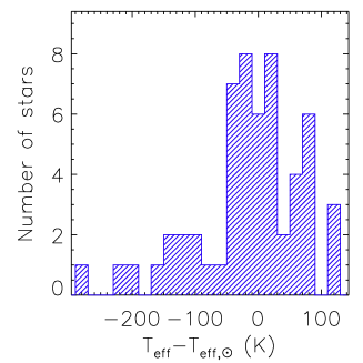
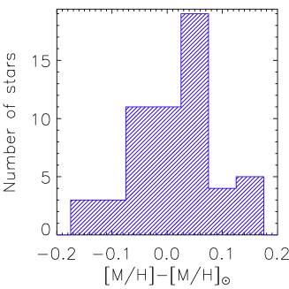
Figure 1: Histograms of the differences between the atmospheric parameters of the twin candidates and of the Sun, as obtained by iSpec.

5 Li content

It is known that the lithium abundances of solar type stars show a large dispersion (see for instance the comprehensive study by Takeda et al., 2007). This is subject to various interpretations. The Sun is depleted in Li and it is expected that solar twins show the same deficiency. We have classified our targets stars into three categories after a visual inspection of the wavelength range inluding the Li lines at $\sim$670.78 nm in comparison to one of the ELODIE solar spectra. We classified into A in Table 2 the stars which show a similar Li deficiency as the Sun, into B those with a slightly higher Li abundance and into C those which exhibit a pronounced Li feature. There are 24, 11 and 21 stars in categories A, B and C respectively. Figure 2 shows two examples of stars in each category. It is worth to note that HIP076114 and HIP088194 are classified A for their similarity to the Sun in both atmospheric parameters and Lithium content.

Stellar rotation and activity are strongly correlated with the surface Li content of solar type stars (Takeda et al., 2007). The stars examined here are supposedly slow rotators due to our initial constraint FWHM $\leq$ 12 km s^-1. It is thus interesting to find so diverse strengths of their Li feature.

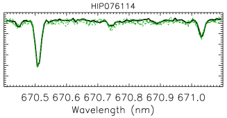
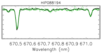
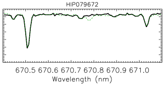
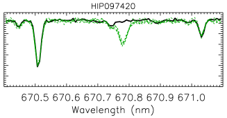
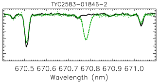
Figure 2: Comparison of the spectral range centered on the 670.78 nm Li feature in one of the Sun spectra (black thick line) and a target (green dashed line), with up to 5 spectra available for some stars. The upper panels show two stars classified A (same Li deficiency as the Sun), the middle panels show two stars classified B (slightly more abundant in Li than the Sun), the bottom panels show two stars classified C (pronounced Li feature).

6 Abundances

The chemical abundances were derived with iSpec and the line list of the Gaia ESO survey, this time including also lines labeled to be less reliable, due to uncertain atomic data or possible blends. However the 18 solar spectra allowed us to keep only the lines which gave consistent abundances from one spectrum to another. Moreover since we are dealing with solar twins, a differential analysis with respect to solar spectra was possible, reducing the uncertainty in relative abundances due to bad atomic data. In that way we were able to obtain a high precision, which is so important to identify solar twins (Meléndez et al., 2012).

A total of 1865 lines were measurable in the ELODIE spectra out of which were kept only those measured in at least 17 out of 18 solar spectra with a weighted standard deviation lower than 0.02. Then we selected the chemical elements for which at least 3 such lines were measured. This left us with 189 Fe lines, 23 Ni lines, 15 Si and Ca lines, 8 Cr lines, 5 Mn and Ti lines, 4 Na lines, all neutral, plus 3 Fe$\rm{II}$ lines. Table 7 lists these 267 lines which were found to be suitable for spectral synthesis of solar type stars. For each of these lines, we took as reference abundance the weighted mean obtained on the 17 or 18 solar spectra. The line by line abundances of the 225 spectra were then measured differentially for this set. As the total error for a line abundance relative to the Sun, we quadratically summed the weighted standard deviation obtained for the solar spectra and the rms of the fit obtained for the target spectrum. Then the weighted average and standard deviation were computed for each element and each star, as presented in Tables 4, 5 and 6. With up to 5 spectra available for a large fraction of the targets, the determination of [Fe$\rm{I}$/H] was often based on the measurement of 945 individual lines. In total we obtained 59 707 individual line measurements with errors between 0.01 and 0.111 and a median error of 0.02. As a verification, we checked the agreement of the [Fe$\rm{I}$/H] and [Fe$\rm{II}$/H] determinations (Fig. 3). The mean difference is 0.008, demonstrating the excellent agreement of the 2 determinations of iron abundances, with a standard deviation of 0.019, agreeing perfectly with the median error of 0.02 of all the individual line measurements.

Fig. 3 also shows that there is a concentration of stars slightly more metal-rich than the Sun, a possible bias of the content of the ELODIE archive in favour of stars followed-up for the search of extra-solar planets.

Figure 3: Difference of iron abundances obtained with neutral and ionised lines for the 56 twin candidates. The mean difference is 0.008 dex with a standard deviation of 0.019 dex.

HIP079672 (18 Sco) has been studied at very high resolution (R $\sim$ 110 000) and S/N (800 - 1000) by Meléndez et al. (2014a) who obtained abundances differentially to the Sun with an unprecedented level of precision. We compare their determinations to ours in Table 3 : they agree within 0.03 for Ti and Cr, within 0.008 for Na and Ca and within 0.004 for Fe, Si, Mn and Ni. Thus the agreement is largely better than expected from our quoted errors. For comparison we also show the abundances from Jofré et al. (2015) who made an extensive study of the Gaia benchmark stars. They are also in excellent agreement.

Table 3: Comparison of abundances determined in this work for HIP079672 (18 Sco) to those obtained by Meléndez et al. (2014a) and by Jofré et al. (2015).

[X/H]	This work	Meléndez et al. (2014a)	Jofré et al. (2015)
Fe	0.051$\pm$0.026	0.054$\pm$0.005	0.03$\pm$ 0.01 (a)
Na	0.017$\pm$0.045	0.025$\pm$0.004
Si	0.043$\pm$0.014	0.047$\pm$0.003	0.048$\pm$ 0.018
Ca	0.065$\pm$0.016	0.057$\pm$0.006	0.058$\pm$ 0.036
Ti	0.022$\pm$0.045	0.051$\pm$0.007	0.046$\pm$ 0.026
Cr	0.034$\pm$0.026	0.056$\pm$0.006	0.049$\pm$ 0.023
Mn	0.037$\pm$0.012	0.041$\pm$0.006	0.040$\pm$ 0.018
Ni	0.038$\pm$0.027	0.041$\pm$0.004	0.039$\pm$ 0.017

Seven solar analogs have all the tested elements agreeing with the solar abundances within 0.05 : HIP021436, HIP035265, HIP076114, HIP085244, HIP089474, HIP100963, TYC2694-00364-1.

Figure 4 shows the iron abundances of the 56 targets from neutral and ionized lines and Fig. 5 displays the abundances of the other elements. The stars are numbered from 1 to 56 for the sake of clarity. The abundances of the tested elements are quite well centered on the solar value, with a small spread. This suggests that the solar abundance pattern is not unusual as suggested by some studies (Nissen, 2015). This point needs however further confirmation with other elements which are not part of this study because of our strict selection of lines very well measured in the ELODIE solar spectra, which has guaranteed a high level of precision.

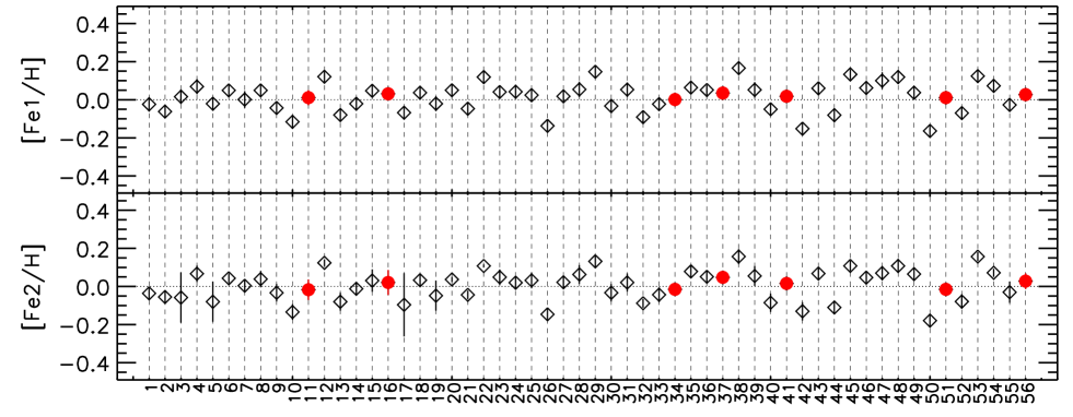
Figure 4: Iron abundance of the 56 solar twin candidates, obtained from neutral and ionized lines. Red dots represent the 7 stars found to have the same abundances than the Sun, within 0.05 dex, for all the tested elements.

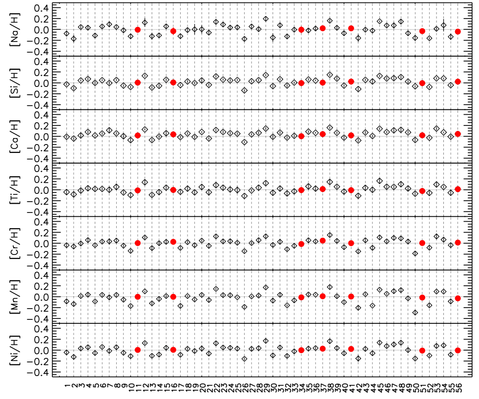
Figure 5: Like Fig. 4 for the other elements.

Table 4: Detailed abundances of the 56 targets

num	HIP/TYC	[Fe$\rm{I}$/H]			[Fe$\rm{II}$/H]			[Na/H]
		Mean	$\sigma$	N	Mean	$\sigma$	N	Mean	$\sigma$	N
1	HIP001813	-0.024	0.038	928	-0.036	0.029	15	-0.076	0.052	16
2	HIP004290	-0.062	0.032	938	-0.055	0.036	15	-0.171	0.067	17
3	HIP007339	0.016	0.038	185	-0.058	0.132	3	0.044	0.028	3
4	HIP007585	0.069	0.039	926	0.067	0.043	15	0.032	0.044	15
5	HIP007902	-0.021	0.036	187	-0.080	0.105	3	-0.112	0.041	4
6	HIP007918	0.049	0.028	944	0.043	0.024	15	0.055	0.031	20
7	HIP011253	0.001	0.044	940	0.004	0.028	15	0.094	0.054	19
8	HIP011728	0.049	0.033	376	0.039	0.043	6	0.045	0.026	8
9	HIP018413	-0.043	0.035	939	-0.033	0.046	15	-0.015	0.044	18
10	HIP021010	-0.116	0.037	940	-0.134	0.041	15	-0.126	0.042	20
11	HIP021436	0.011	0.039	939	-0.017	0.053	15	-0.006	0.047	18
12	HIP024813	0.121	0.028	187	0.124	0.018	3	0.126	0.080	4
13	HIP029432	-0.080	0.033	933	-0.080	0.047	15	-0.125	0.065	16
14	HIP029525	-0.021	0.035	939	-0.012	0.035	15	-0.109	0.040	19
15	HIP031965	0.047	0.035	935	0.031	0.059	15	0.056	0.043	20
16	HIP035265	0.031	0.033	934	0.021	0.065	15	-0.032	0.068	20
17	HIP036874	-0.068	0.035	366	-0.096	0.166	6	-0.124	0.039	8
18	HIP041484	0.037	0.028	940	0.033	0.034	15	-0.011	0.044	18
19	HIP041844	-0.021	0.039	938	-0.048	0.079	15	0.002	0.097	20
20	HIP042575	0.050	0.031	186	0.037	0.013	3	0.003	0.078	4
21	HIP043557	-0.047	0.033	189	-0.044	0.023	3	-0.059	0.044	4
22	HIP043726	0.119	0.028	188	0.108	0.008	3	0.139	0.040	4
23	HIP044089	0.041	0.032	943	0.049	0.040	15	0.090	0.039	19
24	HIP049756	0.042	0.037	938	0.020	0.034	15	0.034	0.047	18
25	HIP050316	0.024	0.034	934	0.032	0.041	15	0.038	0.045	20
26	HIP050505	-0.137	0.029	945	-0.146	0.033	15	-0.174	0.039	21
27	HIP053721	0.018	0.030	940	0.022	0.030	15	0.054	0.037	20
28	HIP056832	0.054	0.040	938	0.063	0.049	15	0.005	0.041	20
29	HIP062527	0.147	0.033	940	0.132	0.033	15	0.195	0.038	19
30	HIP063636	-0.033	0.037	941	-0.033	0.046	15	-0.149	0.076	20
31	HIP064150	0.053	0.038	939	0.021	0.047	15	0.076	0.050	20
32	HIP065721	-0.091	0.033	939	-0.088	0.023	15	-0.129	0.044	19
33	HIP072043	-0.023	0.035	942	-0.043	0.039	15	-0.004	0.047	19
34	HIP076114	0.001	0.035	928	-0.015	0.030	15	-0.005	0.063	18
35	HIP077052	0.064	0.033	942	0.079	0.030	15	-0.018	0.046	20
36	HIP079672	0.051	0.026	188	0.051	0.032	3	0.017	0.045	4
37	HIP085244	0.035	0.034	188	0.048	0.010	3	0.021	0.031	4
38	HIP085810	0.166	0.033	923	0.157	0.039	15	0.160	0.027	18
39	HIP086193	0.052	0.040	923	0.055	0.052	15	0.030	0.045	18
40	HIP088194	-0.050	0.034	945	-0.085	0.048	15	-0.070	0.040	20
41	HIP089474	0.018	0.031	925	0.016	0.022	15	0.020	0.029	18
42	HIP090355	-0.152	0.033	566	-0.130	0.048	9	-0.158	0.071	12
43	HIP094981	0.060	0.032	945	0.068	0.028	15	-0.004	0.032	20
44	HIP096402	-0.081	0.036	377	-0.110	0.029	6	-0.022	0.042	8
45	HIP096895	0.133	0.026	184	0.108	0.027	3	0.149	0.016	3
46	HIP096901	0.062	0.036	374	0.047	0.030	6	0.073	0.031	6
47	HIP096948	0.100	0.044	555	0.070	0.038	9	0.073	0.057	11
48	HIP097336	0.119	0.037	941	0.108	0.037	15	0.144	0.041	18
49	HIP097420	0.037	0.033	936	0.065	0.033	15	-0.070	0.036	17
50	HIP097767	-0.164	0.033	940	-0.179	0.036	15	-0.156	0.055	19
51	HIP100963	0.011	0.034	946	-0.015	0.031	15	-0.031	0.034	20
52	HIP102040	-0.070	0.030	932	-0.079	0.038	15	-0.161	0.022	17
53	HIP116613	0.124	0.034	944	0.157	0.024	15	0.011	0.030	19
54	HIP118162	0.073	0.029	378	0.072	0.021	6	0.077	0.113	8
55	TYC2583-01846-2	-0.027	0.028	943	-0.030	0.056	15	-0.135	0.058	19
56	TYC2694-00364-1	0.027	0.033	933	0.028	0.041	15	-0.040	0.022	15

Table 5: Detailed abundances of the 56 targets

num	HIP/TYC	[Si/H]			[Ca/H]			[Ti/H]
		Mean	$\sigma$	N	Mean	$\sigma$	N	Mean	$\sigma$	N
1	HIP001813	-0.026	0.024	75	-0.008	0.031	75	-0.042	0.049	25
2	HIP004290	-0.097	0.030	75	-0.041	0.025	75	-0.084	0.054	25
3	HIP007339	0.044	0.018	15	0.016	0.038	15	-0.014	0.039	5
4	HIP007585	0.072	0.030	75	0.080	0.029	75	0.028	0.046	25
5	HIP007902	0.000	0.034	15	0.016	0.020	15	0.016	0.032	5
6	HIP007918	0.049	0.016	75	0.052	0.026	75	0.016	0.026	25
7	HIP011253	-0.003	0.033	75	0.111	0.041	75	0.001	0.061	25
8	HIP011728	0.052	0.022	30	0.054	0.025	30	0.053	0.060	10
9	HIP018413	-0.050	0.021	75	0.002	0.043	75	-0.049	0.029	25
10	HIP021010	-0.075	0.026	75	-0.069	0.038	75	-0.097	0.039	25
11	HIP021436	0.005	0.030	75	0.016	0.031	75	-0.011	0.043	25
12	HIP024813	0.130	0.021	15	0.126	0.018	15	0.138	0.045	5
13	HIP029432	-0.084	0.026	74	-0.068	0.027	75	-0.093	0.033	25
14	HIP029525	-0.054	0.026	75	-0.005	0.026	75	-0.042	0.051	25
15	HIP031965	0.058	0.026	75	0.057	0.040	75	0.039	0.037	25
16	HIP035265	0.008	0.025	75	0.036	0.023	75	-0.003	0.029	25
17	HIP036874	-0.040	0.017	28	-0.014	0.029	28	-0.037	0.033	10
18	HIP041484	0.026	0.022	75	0.053	0.024	75	0.022	0.044	25
19	HIP041844	-0.003	0.026	75	-0.010	0.033	75	-0.047	0.043	25
20	HIP042575	0.045	0.038	15	0.080	0.016	15	0.052	0.047	5
21	HIP043557	-0.036	0.022	15	-0.039	0.021	15	-0.045	0.064	5
22	HIP043726	0.118	0.024	15	0.116	0.022	15	0.086	0.040	5
23	HIP044089	0.060	0.020	75	0.080	0.028	75	0.039	0.040	26
24	HIP049756	0.045	0.026	75	0.058	0.030	75	0.006	0.047	25
25	HIP050316	0.052	0.019	75	0.049	0.026	75	-0.004	0.066	25
26	HIP050505	-0.138	0.023	75	-0.106	0.021	75	-0.113	0.031	25
27	HIP053721	0.030	0.017	75	0.036	0.021	75	-0.012	0.024	25
28	HIP056832	0.050	0.027	75	0.065	0.031	75	0.039	0.047	25
29	HIP062527	0.142	0.022	75	0.143	0.027	75	0.122	0.037	25
30	HIP063636	-0.059	0.030	75	-0.008	0.035	75	-0.054	0.057	25
31	HIP064150	0.067	0.024	75	0.068	0.027	75	0.023	0.044	25
32	HIP065721	-0.048	0.026	75	-0.023	0.028	75	-0.066	0.043	25
33	HIP072043	0.005	0.020	75	0.009	0.032	75	-0.028	0.042	25
34	HIP076114	-0.004	0.023	74	0.002	0.029	75	-0.006	0.055	25
35	HIP077052	0.062	0.024	75	0.086	0.024	75	0.062	0.048	25
36	HIP079672	0.043	0.014	15	0.065	0.016	15	0.022	0.045	5
37	HIP085244	0.005	0.021	15	0.041	0.028	15	0.013	0.052	5
38	HIP085810	0.149	0.024	74	0.159	0.023	75	0.144	0.040	25
39	HIP086193	0.079	0.032	72	0.065	0.024	74	0.056	0.034	25
40	HIP088194	-0.049	0.023	75	-0.024	0.034	75	-0.032	0.044	25
41	HIP089474	0.024	0.019	74	0.017	0.036	75	-0.007	0.022	25
42	HIP090355	-0.113	0.033	45	-0.075	0.031	45	-0.109	0.039	15
43	HIP094981	0.055	0.022	75	0.071	0.031	75	0.036	0.046	25
44	HIP096402	0.026	0.048	30	0.006	0.026	30	0.000	0.044	10
45	HIP096895	0.128	0.020	15	0.140	0.025	15	0.163	0.046	5
46	HIP096901	0.081	0.029	30	0.078	0.022	30	0.056	0.038	10
47	HIP096948	0.087	0.038	43	0.110	0.039	45	0.053	0.032	15
48	HIP097336	0.106	0.027	75	0.119	0.037	75	0.102	0.055	25
49	HIP097420	0.024	0.028	75	0.073	0.026	75	0.024	0.054	25
50	HIP097767	-0.062	0.021	75	-0.066	0.034	75	-0.071	0.036	25
51	HIP100963	-0.005	0.021	75	0.019	0.026	75	-0.022	0.039	25
52	HIP102040	-0.075	0.020	75	-0.026	0.020	75	-0.057	0.036	25
53	HIP116613	0.083	0.021	75	0.142	0.031	75	0.097	0.043	25
54	HIP118162	0.082	0.017	30	0.073	0.015	30	0.053	0.026	10
55	TYC2583-01846-2	-0.042	0.026	76	-0.006	0.030	75	-0.054	0.046	25
56	TYC2694-00364-1	0.023	0.030	75	0.044	0.031	75	0.011	0.036	25

Table 6: Detailed abundances of the 56 targets

num	HIP/TYC	[Cr/H]			[Mn/H]			[Ni/H]
		Mean	$\sigma$	N	Mean	$\sigma$	N	Mean	$\sigma$	N
1	HIP001813	-0.036	0.037	40	-0.085	0.037	25	-0.041	0.038	115
2	HIP004290	-0.060	0.040	40	-0.134	0.038	25	-0.124	0.040	115
3	HIP007339	-0.004	0.035	8	0.012	0.019	5	0.032	0.032	23
4	HIP007585	0.058	0.038	38	0.038	0.032	25	0.054	0.041	115
5	HIP007902	-0.036	0.024	8	-0.087	0.023	5	-0.052	0.030	23
6	HIP007918	0.031	0.026	40	0.034	0.022	25	0.059	0.024	115
7	HIP011253	0.034	0.059	39	-0.012	0.046	25	-0.013	0.043	115
8	HIP011728	0.049	0.047	16	0.033	0.027	10	0.054	0.035	46
9	HIP018413	-0.045	0.027	40	-0.055	0.029	25	-0.048	0.031	115
10	HIP021010	-0.140	0.027	39	-0.170	0.026	25	-0.110	0.033	115
11	HIP021436	0.003	0.033	39	-0.002	0.026	25	0.004	0.043	115
12	HIP024813	0.106	0.026	8	0.098	0.012	5	0.131	0.022	23
13	HIP029432	-0.089	0.037	40	-0.122	0.027	25	-0.104	0.031	115
14	HIP029525	0.001	0.036	40	-0.040	0.033	25	-0.081	0.037	115
15	HIP031965	0.026	0.034	40	0.012	0.024	25	0.044	0.039	115
16	HIP035265	0.026	0.037	40	-0.002	0.032	26	0.006	0.031	115
17	HIP036874	-0.085	0.030	16	-0.168	0.034	10	-0.085	0.032	46
18	HIP041484	0.019	0.025	40	0.011	0.019	25	0.024	0.026	115
19	HIP041844	-0.035	0.036	39	-0.051	0.027	25	-0.015	0.041	115
20	HIP042575	0.049	0.024	8	0.033	0.025	5	0.030	0.059	23
21	HIP043557	-0.048	0.037	8	-0.061	0.044	5	-0.062	0.039	23
22	HIP043726	0.126	0.034	8	0.143	0.021	5	0.126	0.038	23
23	HIP044089	0.035	0.041	40	0.029	0.027	25	0.049	0.032	115
24	HIP049756	0.037	0.043	40	0.027	0.028	25	0.043	0.038	115
25	HIP050316	0.009	0.030	40	-0.011	0.014	24	0.028	0.040	115
26	HIP050505	-0.145	0.024	39	-0.187	0.027	25	-0.159	0.026	115
27	HIP053721	0.003	0.027	40	0.005	0.017	25	0.024	0.032	115
28	HIP056832	0.057	0.045	40	0.020	0.024	25	0.037	0.038	115
29	HIP062527	0.127	0.043	40	0.170	0.025	25	0.170	0.034	115
30	HIP063636	-0.031	0.049	39	-0.072	0.043	25	-0.096	0.042	115
31	HIP064150	0.027	0.050	40	0.035	0.032	25	0.049	0.040	116
32	HIP065721	-0.109	0.029	40	-0.159	0.018	25	-0.106	0.032	115
33	HIP072043	-0.047	0.035	39	-0.067	0.033	25	-0.022	0.036	115
34	HIP076114	-0.014	0.036	40	-0.012	0.031	25	-0.001	0.035	115
35	HIP077052	0.055	0.041	40	0.041	0.029	25	0.028	0.034	115
36	HIP079672	0.034	0.026	8	0.037	0.012	5	0.038	0.027	23
37	HIP085244	0.048	0.011	8	0.008	0.019	5	0.027	0.034	23
38	HIP085810	0.151	0.033	40	0.177	0.030	25	0.164	0.035	115
39	HIP086193	0.043	0.035	40	0.009	0.027	25	0.039	0.035	115
40	HIP088194	-0.072	0.041	40	-0.100	0.026	25	-0.057	0.032	116
41	HIP089474	0.001	0.026	40	0.003	0.019	25	0.022	0.031	115
42	HIP090355	-0.149	0.029	24	-0.204	0.034	15	-0.152	0.059	69
43	HIP094981	0.055	0.038	40	0.046	0.022	25	0.023	0.033	115
44	HIP096402	-0.084	0.046	16	-0.163	0.018	10	-0.056	0.038	46
45	HIP096895	0.107	0.032	8	0.128	0.017	5	0.138	0.032	23
46	HIP096901	0.035	0.029	16	0.054	0.021	10	0.075	0.033	46
47	HIP096948	0.098	0.050	24	0.101	0.036	15	0.105	0.053	69
48	HIP097336	0.089	0.034	40	0.121	0.039	25	0.136	0.040	115
49	HIP097420	0.031	0.041	39	-0.030	0.030	25	0.001	0.040	115
50	HIP097767	-0.188	0.032	40	-0.291	0.035	25	-0.154	0.029	115
51	HIP100963	0.004	0.047	40	-0.016	0.021	25	-0.008	0.032	115
52	HIP102040	-0.081	0.032	39	-0.158	0.031	25	-0.099	0.027	115
53	HIP116613	0.125	0.054	40	0.095	0.020	25	0.077	0.044	115
54	HIP118162	0.066	0.038	16	0.094	0.022	10	0.087	0.032	46
55	TYC2583-01846-2	-0.035	0.035	40	-0.086	0.039	25	-0.083	0.035	115
56	TYC2694-00364-1	0.012	0.040	40	-0.030	0.024	25	-0.005	0.035	115

Table 7: Selected lines from the Gaia-ESO survey used for the determination of the differental abundances relative to the Sun (excerpt, full version with 267 lines at CDS). The adopted oscillator strength and excitation potential are given for each line, with the reference for loggf. The Gaia-ESO flags indicate whether the line is recommended (Yes/Undecided/No), based on the quality of the atomic data and of the spectral synthesis for the Sun and Arcturus.

wavelength	element	loggf	EP	flags	loggf reference
Å	+ ion		eV
4807.7082	Fe 1	-2.150	3.368	Y-	Ruffoni et al. (2014)
4808.1478	Fe 1	-2.690	3.252	YY	May et al. (1974)
4811.9829	Ni 1	-1.450	3.658	YN	Johansson et al. (2003)
4829.0231	Ni 1	-0.140	3.542	NY	Kurucz (2008)
4844.0135	Fe 1	-2.050	3.547	Y-	O’Brian et al. (1991)
4848.8826	Fe 1	-3.137	2.279	Y-	O’Brian et al. (1991)
4855.6729	Fe 1	-1.700	3.368	Y-	den Hartog et al. (2014)
4871.9281	Fe 1	-2.150	3.252	Y-	O’Brian et al. (1991)

7 Additional information

The 56 twin candidates are either Hipparcos or Tycho stars. We have retrieved informations for them in the XHIP catalogue (Anderson & Francis, 2012) and in Simbad, reported in Table 8. All the stars are within 60 pc from the Sun, their spectral type vary from F8 to G6.5. Their B-V colours and M_v absolute magnitudes span a wide range of values. Ages are provided in form of a probable range, sometimes very large due to the lack of constraint on this fundamental property.

We proceeded like in the previous sections and classified the stars into two categories depending on the similarity of their M_v absolute magnitude and age with the solar ones. Stars with M_v in the range [4.6 – 5.0] are potentially similar to the Sun (M${}_{v_{\odot}}\simeq 4.80$). If their age interval also includes the age of the Sun ($\sim$4.5 Gyr), then such stars are good twin candidates. Fifteen stars were found to be similar to the Sun, based on their absolute magnitude and age range.

Table 8: Data available in the XHIP catalogue for solar twin candidates. For the two Tycho2 stars, the information was retrieved from Simbad. The last column indicates whether the star has an absolute magnitude and an age compatible to those of the Sun (Yes=A, No=C, Possibly if the information is incomplete=B).

HIP/TYC	HD	Dist	SP	B-V	Mv	U	V	W	age[b-age - B-age]	age + Mv
		pc	type	mag	mag	km s-1	km s-1	km s-1	Gyr
HIP001813	HD001832	40.26	F8	0.639	4.55	-7.3	-62.5	-16.7	8.3 [ 6.0 - 10.0 ]	C
HIP004290	HD005294	29.05	G5	0.652	5.09	33.3	-4.5	-14.5	0.2 [ - 4.4 ]	C
HIP007339	HD009407	20.66	G6.5V	0.686	4.94	50.8	-3.9	1.1		B
HIP007585	HD009986	25.62	G2V	0.648	4.73	-1.1	-17.2	19.0	5.4 [ 1.1 - 9.0 ]	A
HIP007902	HD010145	37.22	G5V	0.691	4.85	113.8	-63.7	-20.7	7.3 [ 2.9 - 11.3 ]	A
HIP007918	HD010307	12.74	G1V	0.618	4.43	-38.6	-31.2	-0.1	6.1 [ 3.5 - 8.2 ]	C
HIP011253	HD014874	60.29	G0V	0.665	4.26	16.0	-20.7	-47.9	10.0 [ 8.3 - 11.7 ]	C
HIP011728	HD015632	39.77	G0	0.666	5.03	-24.2	-8.6	16.3	0.8 [ - 6.7 ]	C
HIP018413	HD024409	21.98	G3V	0.698	4.82	34.5	15.3	-5.9	13.2 [ 9.4 - 16.3 ]	C
HIP021010	HD028447	38.54	G5	0.722	3.58	-31.3	-5.5	18.4	7.3 [ 6.7 - 7.8 ]	C
HIP021436	HD029150	32.57	G5	0.685	5.02	6.4	-7.3	0.2	2.6 [ - 8.6 ]	C
HIP024813	HD034411	12.63	G1V	0.630	4.18	-75.7	-35.1	4.4	5.2 [ 3.8 - 6.5 ]	C
HIP029432	HD042618	23.50	G3V	0.642	4.99	62.1	-12.6	11.2	0.2 [ - 4.3 ]	C
HIP029525	HD042807	17.95	G5V	0.663	5.16	3.0	-25.9	-6.6		C
HIP031965	HD047309	40.25	G0	0.672	4.58	-45.6	-41.4	-8.3	12.0 [ 8.4 - 14.1 ]	C
HIP035265	HD056124	27.08	G0	0.631	4.77	-24.5	-20.4	-6.5	0.6 [ - 5.1 ]	A
HIP036874	HD060298	39.06	G2V	0.642	4.41	140.0	-35.6	-48.2	8.7 [ 7.1 - 12.0 ]	C
HIP041484	HD071148	22.25	G1V	0.624	4.58	19.9	-38.9	-22.7	7.6 [ 4.0 - 9.8 ]	C
HIP041844	HD071881	41.25	G1V	0.630	4.36	-33.3	-60.9	-4.6	6.8 [ 4.8 - 8.4 ]	C
HIP042575	HD073393	39.86	G3V	0.675	5.00	-74.2	-54.4	-12.6	7.2 [ 0.8 - 12.7 ]	A
HIP043557	HD075767	24.00	G0V	0.640	4.67	17.9	-26.7	6.1	9.8 [ 5.5 - 11.0 ]	C
HIP043726	HD076151	17.38	G3V	0.661	4.81	-40.5	-19.8	-11.7	7.1 [ 3.1 - 11.0 ]	A
HIP044089	HD076752	38.50	G2V	0.680	4.54	7.1	-20.2	-20.9	8.5 [ 6.1 - 10.4 ]	C
HIP049756	HD088072	34.91	G3V	0.647	4.83	-19.6	4.5	-32.4	3.7 [ - 7.9 ]	A
HIP050316	HD088986	33.18	G2V	0.635	3.86	-19.1	-21.5	17.5	6.5 [ 4.2 - 7.4 ]	C
HIP050505	HD089269	20.24	G6V	0.653	5.13	12.6	-27.5	1.7	7.7 [ 1.3 - 13.8 ]	C
HIP053721	HD095128	14.06	G1V	0.624	4.29	-24.2	-2.5	0.8	6.8 [ 4.9 - 8.1 ]	C
HIP056832	HD101242	35.04	G6	0.710	4.88	-41.1	-48.9	-1.4	2.7 [ - 7.1 ]	A
HIP062527	HD111513	38.08	G1V	0.633	4.46	-85.8	-51.4	-28.7	6.9 [ 4.9 - 9.0 ]	C
HIP063636	HD113319	31.09	G4V	0.655	5.05	-27.5	-9.8	7.0	7.0 [ - 12.2 ]	C
HIP064150	HD114174	26.12	G3IV	0.667	4.69	57.2	-64.8	-9.5	8.8 [ 6.1 - 11.3 ]	C
HIP065721	HD117176	17.99	G5V	0.714	3.70	12.9	-51.4	-4.3	8.0 [ 7.5 - 8.6 ]	C
HIP072043	HD129814	41.09	G5V	0.636	4.45	15.1	-30.2	5.8	8.4 [ 6.1 - 10.2 ]	C
HIP076114	HD138573	30.24	G5IV-V	0.656	4.82	-36.6	8.8	-19.2	7.1 [ 2.6 - 11.3 ]	A
HIP077052	HD140538	14.66	G5V	0.684	5.03	18.1	-7.3	10.7	2.8 [ - 8.3 ]	C
HIP079672	HD146233	13.90	G2V	0.652	4.77	27.1	-14.4	-22.1	2.4 [ - 6.8 ]	A
HIP085244	HD158222	41.54	G0	0.667	4.73	-18.4	-10.9	-5.2	10.2 [ 6.9 - 12.4 ]	C
HIP085810	HD159222	23.92	G1V	0.639	4.63	-31.0	-49.9	-1.9	4.3 [ 1.3 - 7.8 ]	A
HIP086193	HD159909	35.18	G5	0.693	4.55	-59.0	-54.4	-7.7	13.0 [10.8 - 15.3 ]	C
HIP088194	HD164595	28.35	G2V	0.635	4.81	-17.7	2.3	24.0	10.7 [ 6.6 - 13.6 ]	C
HIP089474	HD168009	22.82	G1V	0.641	4.51	-4.5	-62.1	-22.7	9.1 [ 7.4 - 12.6 ]	C
HIP090355	HD169822	28.84	G6V	0.699	5.53	28.5	-65.3	-6.6		C
HIP094981	HD181655	25.39	G5V	0.676	4.27	22.4	-5.7	-2.5	10.4 [ 8.7 - 11.9 ]	C
HIP096402	HD184768	38.56	G5 V	0.675	4.62	24.8	-61.4	-27.9	14.4 [11.9 - 16.7 ]	C
HIP096895	HD186408	21.08	G1.5V	0.643	4.37	17.4	-30.5	-0.5	7.1 [ 5.3 - 9.7 ]	C
HIP096901	HD186427	21.21	G3V	0.661	4.62	17.2	-30.5	-2.1	7.6 [ 4.7 - 9.5 ]	C
HIP096948	HD186104	41.19	G5 V	0.664	4.57	-53.7	-39.8	-21.2	8.2 [ 5.7 - 10.2 ]	C
HIP097336	HD187123	48.22	G2V	0.661	4.41	3.1	-15.4	-43.8	5.0 [ 3.0 - 6.8 ]	C
HIP097420	HD187237	26.24	G2IV-V	0.660	4.78	-35.5	-19.6	14.2	8.6 [ 4.5 - 12.1 ]	A
HIP097767	HD187923	26.61	G0 V	0.642	4.03	33.2	-51.1	19.3	10.9 [10.0 - 11.8 ]	C
HIP100963	HD195034	28.22	G5	0.642	4.84	24.1	-15.9	-15.5	7.6 [ 3.0 - 11.6 ]	A
HIP102040	HD197076	20.94	G1V	0.611	4.82	-42.9	-15.2	16.3	5.5 [ 0.2 - 9.3 ]	A
HIP116613	HD222143	23.33	G3V	0.665	4.74	-34.1	-15.9	-12.3	6.2 [ 2.0 - 9.7 ]	A
HIP118162	HD224465	24.52	G4V	0.694	4.77	-4.9	8.8	27.5	6.3 [ 1.5 - 9.5 ]	A
TYC2583-01846-2	HD146362	22.22	G1V	0.621	5.00	-9	-33	7		B
TYC2694-00364-1	HD197310			0.60						B

We have also searched in Simbad whether the twin candidates have a detected extrasolar planet and found 4 such stars : HIP053721, HIP065721, HIP096901, HIP097336, none of them being a good solar twin.

8 Discussion

In each of the previous sections, we have classified 56 twin candidates according to their similarity with the Sun using different properties : global spectrum, atmospheric parameters, Li content, abundances of 8 chemical elements, absolute magnitude, age, presence of a planet. According to the TGMET method, 6 stars were found to have a spectrum very similar to that of the Sun : HIP079672, HIP018413, HIP076114, HIP089474, HIP118162, HIP041484. Three stars were found to have solar atmospheric parameters : HIP076114, HIP085244 and HIP088194, two of which with also the same Li deficiency : HIP076114, HIP088194. Seven stars were found to have the solar abundance pattern for 8 chemical elements : HIP021436, HIP035265, HIP076114, HIP085244, HIP089474, HIP100963, TYC2694-00364-1. Table 9 summarizes the categories A, B and C that we gave to each target according to its similarity to the Sun in atmospheric parameters, abundances, Li content, absolute magnitude and age.

Table 9: Summary of the classification of solar twin candidates after comparison to the Sun based on atmospheric parameters, abundances of 8 elements, Li content, absolute magnitude and age. The best solar twins are sorted at the top of the table. The columns AP (atmospheric parameters), Li and Mv+age report the classification (A, B, C) from Tables 2 and 8. The column Ab. indicates whether the differential abundances in Table 4,5, 6 agree with the solar value within 0.05 dex (A) or within 0.10 dex (B), or differ (C). For the 19 stars considered as good solar twins (AP and Ab. equal A or B), the last column indicates studies where that star was previously identified as solar twin : [1] = Soubiran & Triaud (2004), [2] = Meléndez et al. (2006), [3] = Ramírez et al. (2009), [4] = Takeda & Tajitsu (2009), [5] = Datson et al. (2012), [6] = Porto de Mello et al. (2014), [7] = Ramírez et al. (2014b), [8] = Datson et al. (2015)

HIP/TYC	HD	AP	Ab.	Li	Mv+age	previous studies
solar twins
HIP076114	HD138573	A	A	A	A	[5], [6], [7]
HIP085244	HD158222	A	A	B	C	[6]
HIP088194	HD164595	A	B	A	C	[6]
HIP021436	HD029150	B	A	A	C	[8]
HIP035265	HD056124	B	A	C	A	[2]
HIP100963	HD195034	B	A	C	A	[3], [4]
TYC2694-00364-1	HD197310	B	A	C	B
HIP042575	HD073393	B	B	A	A
HIP056832	HD101242	B	B	A	A
HIP118162	HD224465	B	B	A	A
HIP011728	HD015632	B	B	A	C	[6], [8]
HIP018413	HD024409	B	B	A	C
HIP049756	HD088072	B	B	B	A	[1], [6], [7], [8]
HIP079672	HD146233	B	B	B	A	[1], [2], [3], [4], [5], [6], [7], [8]
HIP043557	HD075767	B	B	B	C	[8]
HIP007585	HD009986	B	B	C	A	[2], [6], [7], [8]
HIP097420	HD187237	B	B	C	A	[6]
HIP041484	HD071148	B	B	C	C	[1], [2]
HIP094981	HD181655	B	B	C	C
other stars
HIP011253	HD014874	B	C	B	C
HIP029432	HD042618	B	C	B	C
HIP102040	HD197076	B	C	C	A
HIP007339	HD009407	C	A	A	B
HIP089474	HD168009	C	A	A	C
HIP001813	HD001832	C	B	A	C
HIP031965	HD047309	C	B	A	C
HIP044089	HD076752	C	B	A	C
HIP064150	HD114174	C	B	A	C
HIP072043	HD129814	C	B	A	C
HIP086193	HD159909	C	B	A	C
HIP041844	HD071881	C	B	B	C
HIP077052	HD140538	C	B	B	C
HIP096901	HD186427	C	B	B	C	star with planet
HIP007918	HD010307	C	B	C	C
HIP050316	HD088986	C	B	C	C
HIP053721	HD095128	C	B	C	C	star with planet
HIP007902	HD010145	C	C	A	A
HIP036874	HD060298	C	C	A	C
HIP050505	HD089269	C	C	A	C
HIP090355	HD169822	C	C	A	C
HIP096402	HD184768	C	C	A	C
HIP096895	HD186408	C	C	A	C
HIP097336	HD187123	C	C	A	C	star with planet
HIP097767	HD187923	C	C	A	C
HIP062527	HD111513	C	C	B	C
HIP096948	HD186104	C	C	B	C
HIP043726	HD076151	C	C	C	A
HIP085810	HD159222	C	C	C	A
HIP116613	HD222143	C	C	C	A
TYC2583-01846-2	HD146362	C	C	C	B
HIP004290	HD005294	C	C	C	C
HIP021010	HD028447	C	C	C	C
HIP024813	HD034411	C	C	C	C
HIP029525	HD042807	C	C	C	C
HIP063636	HD113319	C	C	C	C
HIP065721	HD117176	C	C	C	C	star with planet

It is remarkable to find a star similar to the Sun in all these properties : HIP076114 (HD138573), supported also by the absolute magnitude and most probable age range. This star is also in the list of best twins by Datson et al. (2012) although they classifiy it after HIP079672 (18 Sco) (see also Datson et al., 2015). HIP076114 is also part of the survey of solar twin stars within 50 parsecs of the Sun by Porto de Mello et al. (2014), as well as in the Solar Twin Planet Search by Ramírez et al. (2014b), but not mentioned as a remarkable twin in these two papers. It is worth noting that the galactic velocity of that star differs by $\sim$40 km s^-1 from that of the Sun, suggesting that it is not a solar sibling. It is however an excellent star to use for calibrations or to search for exoplanets.

HIP085244 is our second best twin candidate, with solar atmospheric parameters and chemical pattern but it is classified B for the Li, with a slightly more enhanced content. According to XHIP this star is supposed to be older than the Sun. HIP085244 is also part of the survey of solar twin stars within 50 parsecs of the Sun by Porto de Mello et al. (2014).

HIP088194 has solar atmospheric parameters and is deficient in Li, but it is slightly more metal-poor than the Sun. This is clearly visible in the Figures 4 and 5 (star 40). It is older than the Sun according to XHIP, but of the same age according to Porto de Mello et al. (2014). It is one of the new candidates considered as excellent in that work.

HIP021436 has the solar chemical pattern, and also the same Li content but its effective temperature is lower by $\sim$60 K than that of the Sun. Despite us classifying it B for the atmospheric parameters, it still falls into the solar twin category according to the criterion defined by Meléndez et al. (2014b). Our T_eff determination (5715$\pm$10 K) is in very good agreement with the 7 values listed in the PASTEL catalog (Soubiran et al., 2010) ranging from 5675 to 5748 K. It is worth noting that this star has a galactic velocity compatible with that of the Sun within 10 km s^-1. Its age reported in XHIP is not well constrained, so possibly compatible with that of the Sun. It is thus also a very good solar sibling candidate.

HIP035265 has the solar chemical pattern, an absolute magnitude and age compatible with the Sun, but it is hotter by $\sim$80 K and with a strong Li feature. It also has a galactic velocity different from the Sun. This is thus neither a perfect solar twin or sibling.

HIP100963 has the solar chemical pattern, but it is hotter than the Sun (T_eff= 5821$\pm$6 K) and has a pronounced Li feature. It was previously identified as solar twin by Ramírez et al. (2009) who determined T_eff= 5815 K and [Fe/H]=+0.018$\pm$0.019 in very good agreement with our determinations (we determined [Fe/H]=+0.011$\pm$0.034). Considering this star as an excellent solar twin, Takeda & Tajitsu (2009) made an extensive study at very high resolution (R=90 000) and high S/N (500-1000) and found it hotter than the Sun by 23 K, with a difference of iron abundance of 0.004 and a higher Li content by a factor of $\sim$56 as compared to Sun, also in good agreement with our findings.

TYC2694-00364-1 has been poorly studied as an individual star until now. It essentially differs from the Sun by its hotter temperature (T_eff= 5842$\pm$1 K) and a strong Li feature.

HIP042575, HIP056832 and HIP118162 are our next good solar twins, never identified as such before. Although slightly metal-rich, their abundances differ by less than 0.1 dex from those of the Sun. They exhibit the solar Li deficiency and have an age and absolute magnitude compatible with those of the Sun. Next is HIP011728, also more metal-rich but previously identified as solar twin by Porto de Mello et al. (2014) and Datson et al. (2015). Its absolute magnitude is reported as Mv=5.03 in XHIP, higher than that of the Sun. Then we have HIP018413, a new solar twin, slightly colder, more metal-poor and older than the Sun, which was one of the closest twins according to TGMET. HIP049756 was already identified as a solar twin in several previous studies. We classified it B for the atmospheric parameters and abundances because of [M/H] and [Ca/H] being slightly higher than our limits, 0.05 dex and 0.058 dex respectively, while all the other values are solar. Its main difference to the Sun is a higher lithium content.

The most studied HIP079672 (18 Sco) is definitively not a perfect solar twin, according to our ranking at the 14th position in Table 9. We find a hotter temperature and enhanced abundances relative to the Sun, including the lithium, thus confirming the findings of Meléndez et al. (2014a).

The next four solar twins are already known. They have all a higher lithium content. The last one of the list, HIP094981, is unknown. It is colder and more metal rich but still a solar twin according to the criterion of Meléndez et al. (2014b). It is also more luminous (Mv=4.27) and much older than the Sun (10.4 Gyr) with a strong Li feature.

The second part of Table 9 lists the other stars which were found to differ from the Sun, either in their atmospheric parameters or in their abundances. It is however worth to note HIP007339 and HIP089474 which have the solar chemical pattern and lithium deficiency. HIP007339 is one of the coldest star of our sample (T_eff=5630$\pm$12 K) while HIP089474 differs from the Sun by its lower surface gravity ($\log$ g= 4.29$\pm$0.01). Both stars are not however good solar sibling candidates, having a galactic velocity significantly different from the Sun, with a radial velocity component U=50.8 km s^-1for HIP007339 and a rotational component V= -62.1 km s^-1for HIP089474. HIP089474 is also old (9.1 Gyr), which interestingly makes it a possible member of the thick disk.

9 Conclusion

In this work, we have selected 56 solar twin candidates, among 1165 tested stars, based on the similarity of their spectrum to that of the Sun. We have determined their atmospheric parameters and abundances, and examined their Li content to further study their similarity to the Sun.

A strength of our study is that we have used as reference a large number of solar spectra (18), representive of the range of observing conditions, and from which we have selected the best lines to be analyzed for abundance measurements by synthesis. Several spectra were available for the majority of the selected targets, up to 5 (225 spectra in total). The analysis was performed differentially to the solar spectra, on a line by line basis for the selected set of lines. This led to a very good internal precision. Our atmospheric parameters and abundances proved to also be accurate, in excellent agreement with other studies made at higher resolution and S/N. This demonstrates that the ELODIE archive is a very good resource to make comprehensive studies of solar type stars.

We found that the best solar twin in our sample is HIP076114 (HD138573), dethroning previous candidates (HIP079672/18 Sco, HIP100963). All the other stars slightly differ from the Sun in one or another property. We list 19 solar twins which have T_eff, $\log$ g and abundances differing from those of the Sun by less than 100 K and 0.1 dex respectively.

We found a good solar sibling candidate : HIP021436 which would be worth studying further.