Strongly Monotone Drawings of Planar Graphs

Abstract

A straight-line drawing of a graph is a monotone drawing if for each pair of vertices there is a path which is monotonically increasing in some direction, and it is called a strongly monotone drawing if the direction of monotonicity is given by the direction of the line segment connecting the two vertices.

We present algorithms to compute crossing-free strongly monotone drawings for some classes of planar graphs; namely, 3-connected planar graphs, outerplanar graphs, and 2-trees. The drawings of 3-connected planar graphs are based on primal-dual circle packings. Our drawings of outerplanar graphs depend on a new algorithm that constructs strongly monotone drawings of trees which are also convex. For irreducible trees, these drawings are strictly convex.

1 Introduction

To find a path between a source vertex and a target vertex is one of the most important tasks when data are given by a graph, c.f. Lee et al. [15]. This task may serve as criterion for rating the quality of a drawing of a graph. Consequently researchers addressed the question of how to visualize a graph such that finding a path between any pair of nodes is easy. A user study of Huang et al. [12] showed that, in performing path-finding tasks, the eyes follow edges that go in the direction of the target vertex. This empirical study triggered the research topic of finding drawings with presence of some kind of geodesic paths. Several formalizations for the notion of geodesic paths have been proposed, most notably the notion of strongly monotone paths. Related drawing requirements are studied under the titles of self-approaching drawings and greedy drawings.

Let $G=(V,E)$ be a graph. We say that a path $P$ is monotone with respect to a direction (or vector) $d$ if the orthogonal projections of the vertices of $P$ on a line with direction $d$ appear in the same order as in $P$. A straight-line drawing of $G$ is called monotone if for each pair of vertices $u,v\in V$ there is a connecting path that is monotone with respect to some direction. To support the path-finding tasks it is useful to restrict the monotone direction for each path to the direction of the line segment connecting the source and the target vertex: a path $v_{1}v_{2}\ldots v_{k}$ is called strongly monotone if it is monotone with respect to the vector $\overrightarrow{v_{1}v_{k}}$. A straight-line drawing of $G$ is called strongly monotone if each pair of vertices $u,v\in V$ is connected by a strongly monotone path.

In this paper, we are interested in strongly monotone drawings which are also planar. If crossings are allowed, then any strongly monotone drawing of a spanning tree of $G$ yields a strongly monotone drawing of $G$, this has been observed by Angelini et al. [2].

Related Work.

In addition to (strongly) monotone drawings, there are several other drawing styles that support the path-finding task. The earliest studied is the concept of greedy drawings, introduced by Rao et al. [19]. In a greedy drawing, one can find a source–target path by iteratively selecting a neighbor that is closer to the target. Triangulations admit crossing free greedy drawings [7], and more generally 3-connected planar graphs have greedy drawings [16]. Trees with a vertex of degree at least 6 have no greedy drawing. Nöllenburg and Prutkin [17] gave a complete characterization of trees that admit a greedy drawing.

Greedy drawings can have some undesirable properties, e.g., a greedy path can look like a spiral around the target vertex. To get rid of this effect, Alamdari et al. [1] introduced a subclass of greedy drawings, so-called self-approaching drawings which require the existence of a source–target path such that for any point $p$ on the path the distance to another point $q$ is decreasing along the path. In greedy drawings this is only required for $q$ being the target-vertex. These drawings are related to the concept of self-approaching curves [13]. Alamdari et al. provide a complete characterization of trees that admit a self-approaching drawing.

Even more restricted are increasing-chord drawings, which require that there always is a source–target path which is self-approaching in both directions. Nöllenburg et al. [18] proved that every triangulation has a (not necessarily planar) increasing-chord drawing and every planar 3-tree admits a planar increasing-chord drawing. Dehkordi et al. [6] studied the problem of connecting a given point set in the plane with an increasing-chord graph.

Monotone drawings were introduced by Angelini et al. [2] They showed that any $n$-vertex tree admits a monotone drawing on a grid of size $O(n^{1.6})\times O(n^{1.6})$ or $O(n)\times O(n^{2})$. They also showed that any 2-connected planar graph has a monotone drawing having exponential area. Kindermann et al. [14] improved the area bound to $O(n^{1.5})\times O(n^{1.5})$ even with the property that the drawings are convex. The area bound was further lowered to $O(n^{1.205})\times O(n^{1.205})$ by He and He [9]. Hossain and Rahman [11] showed that every connected planar graph admits a monotone drawing on a grid of size $O(n)\times O(n^{2})$. For 3-connected planar graphs, He and He [10] proved that the convex drawings on a grid of size $O(n)\times O(n)$, produced by the algorithm of Felsner [8], are monotone. For the fixed embedding setting, Angelini et al. [3] showed that every plane graph admits a monotone drawing with at most two bends per edge, and all 2-connected plane graphs and all outerplane graphs admit a straight-line monotone drawing.

Angelini et al. [2] also introduced the concept of strong monotonicity and gave an example of a drawing of a planar triangulation that is not strongly monotone. Kindermann et al. [14] showed that every tree admits a strongly monotone drawing. However, their drawing is not necessarily strictly convex and requires more than exponential area. Further, they presented an infinite class of 1-connected graphs that do not admit strongly monotone drawings. Nöllenburg et al. [18] have recently shown that exponential area is required for strongly monotone drawings of trees and binary cacti.

There are some relations among the aforementioned drawing styles. Plane increasing-chord drawings are self-approaching by definition but also strongly monotone. Self-approaching drawings are greedy by definition. On the other hand, (plane) self-approaching drawings are not necessarily monotone, and vice-versa.

Our Contribution.

After giving some basic definitions used throughout the paper in Section 2, we present four results. First, we show that any 3-connected planar graph admits a strongly monotone drawing induced by primal-dual circle packings (Section 3). Then, we answer in the affirmative the open question of Kindermann et al. [14] on whether every tree has a strongly monotone drawing which is strictly convex. We use this result to show that every outerplanar graph admits a strongly monotone drawing (Section 4). Finally, we prove that 2-trees can be drawn strongly monotone (Section 5). All our proofs are constructive and admit efficient drawing algorithms. Our main open question is whether every planar 2-connected graph admits a plane strongly monotone drawing (Section 6). It would also be interesting to understand which graphs admit strongly monotone drawings on a grid of polynomial size.

2 Definitions

Let $G=(V,E)$ be a graph. A drawing $\Gamma$ of $G$ maps the vertices of $G$ to distinct points in the plane and the edges of $G$ to simple Jordan curves between their end-points. A planar drawing induces a combinatorial embedding which is the class of topologically equivalent drawings. In particular, an embedding specifies the connected regions of the plane, called faces, whose boundary consists of a cyclic sequence of edges. The unbounded face is called the outer face, the other faces are called internal faces. An embedding can also be defined by a rotation system, that is, the circular order of the incident edges around a vertex. Note that both definitions are equivalent for planar graphs.

A drawing of a planar graph is a convex drawing if it is crossing free and internal faces are realized as convex non-overlapping polygonal regions. The augmentation of a drawn tree is obtained by substituting each edge incident to a leaf by a ray which is begins with the edge and extends across the leaf. A drawing of a tree is a (strictly) convex drawing if the augmented drawing is crossing free and has (strictly) convex faces, i.e., all the angles of the unbounded polygonal regions are less or equal to (strictly less than) $\pi$. Note that strict convexity forbids vertices of degree 2. We call a tree irreducible if it contains no vertices of degree 2. It has been observed before that a convex drawing of a tree is also monotone but a monotone drawing is not necessarily convex, see [2, 4].

A $k$-tree is a graph which can be produced from a complete graph $K_{k+1}$ and then repeatedly adding vertices in such a way that the neighbors of the added vertex form a $k$-clique. We say that the new vertex is stacked on the clique. By construction $k$-trees are chordal graphs. They can also be characterized as maximal graphs with treewidth $k$, that is, no edges can be added without increasing the treewidth. Note that $1$-trees are equivalent to trees and $2$-trees are equivalent to maximal series-parallel graphs.

We denote an undirected edge between two vertices $a,b\in V$ by $(a,b)$. In a drawing of $G$, we may identify each vertex with the point in the plane it is mapped to. For two vectors $x$ and $y$, we define the angle $\measuredangle(x,y)$ as the smallest angle between the two vectors, that is, $\measuredangle(x,y)=\arccos\left(\frac{\langle x,y\rangle}{|x||y|}\right)$, and for three points $p,q,r$, we define $\measuredangle{pqr}=\measuredangle(\overrightarrow{qp},\overrightarrow{qr})$. We say that a vector $x$ is monotone with respect to $y$ if $\measuredangle(x,y)<\pi/2$. This yields an alternative definition of a strongly monotone path: A path $v_{1}v_{2}\dots v_{k}$ is strongly monotone if $\measuredangle(\overrightarrow{v_{i}v_{i+1}},\overrightarrow{v_{1}v_{k}})<\pi/2$, for $1\leq i\leq k-1$. Note that we interpret monotonicity as strict monotonicity, i.e., we do not allow edges on the path that are orthogonal to the segment between the endpoints.

3 3-Connected Planar Graphs

In this section, we prove the following theorem.

Theorem 1.

Every 3-connected planar graph has a strongly monotone drawing.

Proof.

We show that the straight-line drawing corresponding to a primal-dual circle packing of a graph $G$ is already strongly monotone. The theorem then follows from the fact that any 3-connected planar graph $G=(V,E)$ admits a primal-dual circle packing. This was shown by Brightwell and Scheinerman [5]; for a comprehensive treatment of circle packings we refer to Stephenson’s book [20].

A primal-dual circle packing of a plane graph $G$ consists of two families ${\cal C}_{V}$ and ${\cal C}_{F}$ of circles such that, there is a bijection $v\leftrightarrow C_{v}$ between the set $V$ of vertices of $G$ and circles of ${\cal C}_{V}$ and a bijection $f\leftrightarrow C_{f}$ between the set $F$ of faces of $G$ and circles of ${\cal C}_{F}$. Moreover, the following properties hold:

1. The circles in the family ${\cal C}_{V}$ are interiorly disjoint and their contact graph is $G$, i.e., $C_{u}\cap C_{v}\neq\emptyset$ if and only if $(u,v)\in E(G)$.

2. If $C_{o}\in{\cal C}_{F}$ is the circle of the outer face $o$, then the circles of ${\cal C}_{F}\setminus\{C_{o}\}$ are interiorly disjoint while $C_{o}$ contains all of them. The contact graph of ${\cal C}_{F}$ is the dual $G^{*}$ of $G$, i.e., $C_{f}\cap C_{g}\neq\emptyset$ if and only if $(f,g)\in E(G^{*})$.

3. The circle packings $C_{V}$ and $C_{F}$ are orthogonal, i.e., if $e=(u,v)$ and the dual of $e$ is $e^{*}=(f,g)$, then there is a point $p_{e}=C_{u}\cap C_{v}=C_{f}\cap C_{g}$; moreover, the common tangents $t_{e^{*}}$ of $C_{u}$, $C_{v}$ and $t_{e}$ of $C_{f}$, $C_{g}$ cross perpendicularly in $p_{e}$.

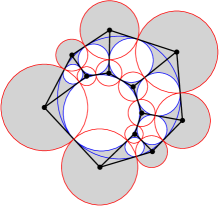
(a)

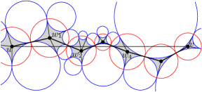
(b)

Figure 1: (a) Drawing $\Gamma$ of 3-connected graph $G=(V,E)$. Red circles are vertex circles $\mathcal{C}_{V}$, Blue circles are face circles $\mathcal{C}_{F}$. Regions of faces in white, regions of vertices in gray. (b) A strongly monotone path (thick edges) from $u$ to $v$.

Let a primal-dual circle packing of a graph $G$ be given. For each vertex $v$, let $p_{v}$ be the center of the corresponding circle $C_{v}$. By placing each vertex $v$ at $p_{v}$, we obtain a planar straight-line drawing $\Gamma$ of $G$. In this drawing, the edge $e=(u,v)$ is represented by the segment with end-points $p_{u}$ and $p_{v}$ on $t_{e}$. The face circles are inscribed circles of the faces of $\Gamma$; moreover, $C_{f}$ is touching each boundary edge of the face $f$; see Figure 1a.

A straight-line drawing $\Gamma^{*}$ of the dual $G^{*}$ of $G$ with the dual vertex of the outer face $o$ at infinity can be obtained similarly by placing the dual vertex of each bounded face $f$ at the center of the corresponding circle $C_{f}$. In this drawing, a dual edge $e^{*}=(f,o)$ is represented by the ray supported by $t_{e^{*}}$ that starts at $p_{f}$ and contains $p_{e}$.

In the following, we will make use of a specific partition $\Pi$ of the plane. The regions of $\Pi$ correspond to the vertices and the faces of $G$. For a vertex or face $x$, let $D_{x}$ be the interior disk of $C_{x}$.

• The region $R_{f}$ of a bounded face $f$ is $D_{f}$.

• The region $R_{v}$ of a vertex $v$ is obtained from the disk $D_{v}$ by removing the intersections with the disks of bounded faces, i.e., $R_{v}=D_{v}\setminus\bigcup_{f\neq o}R_{f}=D_{v}\setminus\bigcup_{f\neq o}D_{f}$; see Figure 1a.

To get a partition of the whole plane, we assign the complement of the already defined regions to the outer face, i.e, $R_{o}=\mathbb{R}^{2}\setminus(\bigcup_{f\neq o}R_{f}\cup\bigcup_{v}R_{v})=\mathbb{R}^{2}\setminus(\bigcup_{f\neq o}D_{f}\cup\bigcup_{v}D_{v}).$

Note that the edge-points $p_{e}$ are part of the boundary of four regions of $\Pi$ and if two regions of $\Pi$ share more than one point on the boundary, then one of them is a vertex region $R_{v}$, the other is a face-region $D_{f}$, and $(v,f)$ is an incident pair of $G$.

We are now prepared to prove the strong monotonicity of $\Gamma$. Consider two vertices $u$ and $v$ and let $\ell$ be the line spanned by $p_{u}$ and $p_{v}$. W.l.o.g., assume that $\ell$ is horizontal and $p_{u}$ lies left of $p_{v}$. Let $\ell_{\text{s}}$ be the directed segment from $p_{u}$ to $p_{v}$. Since $p_{u}\in R_{u}$ and $p_{v}\in R_{v}$, the segment $\ell_{\text{s}}$ starts and ends in these regions. In between, the segment will traverse some other regions of $\Pi$. This is true unless $(u,v)$ is an edge of $G$ whence the strong monotonicity for the pair is trivial. We assume non-degeneracy in the following sense.

Non-degeneracy: The interior of the segment $\ell_{\text{s}}$ contains no vertex-point $p_{w}$, edge-point $p_{e}$, or face-point $p_{f}$.

Möbius transformations of the plane map circle packings to circle packings. In fact the primal-dual circle packing of $G$ is unique up to Möbius transformation, see [20]. Now any degenerate primal-dual circle packing of $G$ can be mapped to a non-degenerate one by a Möbius transformation. This justifies the non-degeneracy assumption. Later we will give a more direct handling of degenerate situations.

Let $u=w_{0},w_{1},\ldots,w_{k}=v$ be the sequence of vertices whose region is intersected by $\ell_{\text{s}}$, in the order of intersection from left to right; see Figure 1b and let $p_{i}=p_{w_{i}}$. We will construct a strongly monotone path $P$ from $p_{u}$ to $p_{v}$ in $\Gamma$ that contains $p_{u}=p_{0},p_{1},\ldots,p_{k}=p_{v}$ in this order. Let $P_{i}$ be the subpath of $P$ from $p_{i-1}$ to $p_{i}$. Since $\ell_{\text{s}}$ may revisit a vertex-region, it is possible that $p_{i-1}=p_{i}$; in this case we set $P_{i}=p_{i}$. Now suppose that $p_{i-1}\neq p_{i}$. Non-degeneracy implies that the segment $\ell_{\text{s}}$ alternates between vertex-regions and face-regions; hence, a unique disk $D_{f}$ is intersected by $\ell_{\text{s}}$ between the regions of $w_{i-1}$ and $w_{i}$. It follows that $w_{i-1}$ and $w_{i}$ are vertices on the boundary of $f$. The boundary of $f$ contains two paths from $w_{i-1}$ to $w_{i}$. In $\Gamma$, one of these two paths from $p_{i-1}$ to $p_{i}$ is above $D_{f}$; we call it the upper path, the other one is below $D_{f}$, this is the lower path. If the center $p_{f}$ of $D_{f}$ lies below $\ell$, we choose the upper path from $p_{i-1}$ to $p_{i}$ as $P_{i}$; otherwise, we choose the lower path.

Figure 2: The path $P_{i}$ connecting $p_{i-1}$ and $p_{i}$.

Suppose that this rule led to the choice of the upper path; see Figure 2. The case that the lower path was chosen works analogously. We have to show that $P_{i}$ is monotone with respect to $\ell$, i.e., to the $x$-axis. Let $e_{1},\ldots,e_{r}$ be the edges of this path and let $e_{j}=(q_{j-1},q_{j})$; in particular $q_{0}=p_{i-1}$ and $q_{r}=p_{i}$. Since $R_{w_{i-1}}$ is star-shaped with center $p_{i-1}$, the segment connecting $p_{i-1}$ with the first intersection point of $\ell$ with $C_{f}$ belongs to $R_{w_{i-1}}$. Therefore, the point $p_{e_{1}}$ of tangency of edge $e_{1}$ at $C_{f}$ lies above $\ell$. Similarly, $p_{e_{r}}$ and, hence, all the points $p_{e_{j}}$ lie above $\ell$. Since the points $p_{e_{1}},\ldots,p_{e_{r}}$ appear in this order on $C_{f}$ and the center of $C_{f}$ lies below $\ell$, we obtain that their $x$-coordinates are increasing in this order. This sequence is interleaved with the $x$-coordinates of $q_{0},q_{1},\ldots,q_{r}$, whence this is also monotone. This proves that the chosen path $P_{i}$ is monotone with respect to $\ell$. Monotonicity also holds for the concatenation $P=P_{1}+P_{2}+\ldots+P_{k}$; see Figure 1b.

We have shown strong monotonicity under the non-degeneracy assumption. Next we consider degenerate cases and show how to find strongly monotone paths in these cases.

If $\ell_{\text{s}}$ contains a vertex-point $p_{w}$ with $w\neq u,v$, the path $P$ between $u$ and $v$ is just the concatenation of monotone paths between the pairs $u,w$ and $w,v$; hence, it is strongly monotone. Next suppose that $\ell_{\text{s}}$ contains an edge-point $p_{e}$. If the edge $e$ in $\Gamma$ is horizontal, then we also have two vertex-points on $\ell_{\text{s}}$ and are in the case described above; otherwise, we consider the region which is touching $\ell$ from above as intersecting and the region which is touching $\ell$ from below as non-intersecting. This recovers the property that there is an alternation between vertex-regions and face-regions intersected by $\ell_{\text{s}}$. Hence, the definition of the path for $u$ and $v$ gives a strongly monotone path unless it contains a vertical edge. The use of a vertical edge can be excluded by properly adjusting degeneracies of the form $p_{f}\in\ell$. For faces $f$ with $p_{f}\in\ell$, we use the upper path, i.e., we consider $p_{f}$ to be below $\ell$. Thus, even in degenerate situations the drawing corresponding to a primal-dual circle packing is strongly monotone. This concludes the proof. ∎

4 Trees and Outerplanar Graphs

Kindermann et al. [14] have shown that any tree has a strongly monotone drawing and that any irreducible binary tree has a strictly convex strongly monotone drawing. They left as an open question whether every tree admits a convex strongly monotone drawing; noticing that, in the positive case, this would imply that every Halin graph has a convex strongly monotone drawing.

In this section, we show that every tree has a convex strongly monotone drawing. Moreover, if the tree is irreducible, then the drawing is strictly convex. We use the result on trees to prove that every outerplanar graphs admits a strongly monotone drawing.

Theorem 2.

Every tree has a convex strongly monotone drawing. If the tree is irreducible, then the drawing is strictly convex.

Proof.

We actually prove something stronger, namely, that any tree $T$ has a drawing $\Gamma$ with the following properties:

1. Every leaf of $T$ is placed on a corner of the convex hull of the vertices in $\Gamma$.

2. If $a_{1},\ldots,a_{\ell}$ is the counterclockwise order of the leaves on the convex hull, then for $i=1,\ldots,\ell$ the vectors $(\overrightarrow{a_{i}a_{i-1}})^{\perp}$, $\overrightarrow{p_{i},a_{i}}$, $(\overrightarrow{a_{i+1}a_{i}})^{\perp}$ appear in counterclockwise radial order, where $p_{i}$ denotes the unique vertex adjacent to $a_{i}$.

3. The angle between two consecutive edges incident to a vertex $v\in V(T)$ is at most $\pi$ and is equal to $\pi$ only when $v$ has degree two.

4. $\Gamma$ is strongly monotone.

Let $T$ be a tree on at least 3 vertices, rooted at some vertex $v_{0}$ with degree at least 2. We inductively produce a drawing of $T$. We begin with placing the root $v_{0}$ at any point in the plane and the children $u_{1},\ldots,u_{k}$ of $v_{0}$ at the corners of a regular $k$-gon with center $v_{0}$. The resulting drawing clearly fulfills the four desired properties.

Let $T^{-}$ be a subtree of $T$ and let $\Gamma^{-}$ be a drawing of $T^{-}$ that fulfills the properties (I1)–(I4). Let $a_{i}$ be a leaf of $T^{-}$ and $u_{1},\dots,u_{k}$ be the children of $a_{i}$ in $T$. Let $T^{+}$ denote the subtree of $T$ induced by $V(T^{-})\cup\{u_{1},\dots,u_{k}\}$. In the inductive step, we explain how to extend the drawing $\Gamma^{-}$ of $T^{-}$ to a drawing $\Gamma^{+}$ of $T^{+}$ such that it fulfills the properties (I1)–(I4).

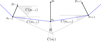
(a)

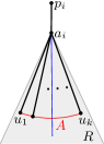
(b)

Figure 3: (a) The region $R$ which is used for placing all the children of vertex $a_{i}$. The boundary of the convex hull is drawn blue. (b) Placement of the children $u_{1},\ldots,u_{k}$ on the arc $A\subset R$. The prolongation $h_{p_{i},a_{i}}$ is drawn blue, the arc $A$ is drawn red.

We first define a region $R$ which is appropriate for the placement of $u_{1},\dots,u_{k}$; see Figure 3a for an illustration. Let $C(a_{i})$ be the open cone containing all points $x$ such that the vectors $(\overrightarrow{a_{i}a_{i-1}})^{\perp}$, $\overrightarrow{a_{i}x}$, and $(\overrightarrow{a_{i+1}a_{i}})^{\perp}$ are ordered counterclockwise. From property (I2), it follows that $C(a_{i})$ contains the prolongation $h_{p_{i},a_{i}}$ of $\overrightarrow{p_{i}a_{i}}$, i.e., the ray that starts with $\overrightarrow{p_{i}a_{i}}$ and extends across $a_{i}$. For every vertex $y\neq a_{i}$ of $T^{-}$, let $C(y)$ be the open cone consisting of all points $p$ such that the path from $y$ to $a_{i}$ in $T^{-}$ is strictly monotone with respect to $\overrightarrow{yp}$. Since the drawing $\Gamma^{-}$ is strongly monotone in a strict sense, $C(y)$ contains an open disk centered at $a_{i}$. We define the region $R$ to be the intersection of all these cones, i.e., $R=\cap_{y\in V(T^{-})}{C(y)}$. The intersection of the cones $\{C(y)\mid y\in V(T^{-})\setminus\{a_{i}\}\}$ contains an open disk centered at $a_{i}$. The intersection of this disk with $C(a_{i})$ yields an open ‘pizza slice’ contained in $R$. In particular, $R$ is non-empty.

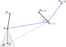
(a)

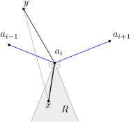
(b)

Figure 4: (a) An illustration for the proof of property (I1) and property (I2). (b) An illustration of the case where $y\in V(T^{-})$ and $x\in\{u_{1},\dots,u_{k}\}$.

Since $R$ is an open convex set, we can construct a circular arc $A$ in $R$ with center $a_{i}$ that contains points on both sides of the prolongation $h_{p_{i},a_{i}}$ of $\overrightarrow{p_{i}a_{i}}$; see Figure 3b. We place the vertices $u_{1},\dots,u_{k}$ on the arc $A$ such that $\measuredangle{p_{i}a_{i}u_{1}}=\measuredangle{u_{k}a_{i}p_{i}}$. This placement implies that in case $a_{i}$ has degree $2$, $\measuredangle{p_{i}a_{i}u_{1}}=\measuredangle{u_{k}a_{i}p_{i}}=\pi$, and otherwise all the angles $\measuredangle{p_{i}a_{i}u_{1}}$, $\measuredangle{u_{k}a_{i}p_{i}}$, $\measuredangle{u_{j}a_{i}u_{j+1}}$, for $j=1,\ldots,k-1$, are all less than $\pi$. This ensures property (I3).

Next, we prove that the drawing $\Gamma^{+}$ of $T^{+}$ fulfills property (I1). We first show that $a_{i-1}$ and $a_{i+1}$ lie on the convex hull of $\Gamma^{+}$; see Figure 4a. Consider the path from $a_{i+1}$ to $a_{i}$ in $T^{-}$, and let $x$ be a point in $R$. By definition of $R$, this path is monotone (in a strict sense) with respect to $\overrightarrow{a_{i}x}$; therefore, $\measuredangle{p_{i+1}a_{i+1}x}<\pi/2$. Considering the strictly monotone path from $a_{i+2}$ to $a_{i+1}$ in $T^{-}$ we obtain that $\measuredangle{a_{i+2}a_{i+1}p_{i+1}}<\pi/2$. The two inequalities above sum up to $\measuredangle{xa_{i+1}a_{i+2}}<\pi$ which means that $a_{i+1}$ lies on the convex hull of $\Gamma^{+}$. Analogously, we obtain that $a_{i-1}$ lies on the convex hull of $\Gamma^{+}$.

Notice that at least one of $u_{1},\ldots,u_{k}$ lies on the convex hull of $\Gamma^{+}$ since they are placed outside of the convex hull of $\Gamma^{-}$. On the other hand, the construction of the circular arc $A$ on which they are placed ensures that all of them lie on the convex hull of $\Gamma^{+}$.

For property (I2), observe that $\measuredangle{xa_{i}a_{i+1}}>\pi/2$ holds for every $x\in C(a_{i})$ (see Figure 4a), and therefore $\measuredangle{a_{i+1}xa_{i}}<\pi/2$, as these two angles lie in the triangle $\triangle xa_{i}a_{i+1}$. The last inequality implies property (I2) for $\Gamma^{+}$.

Finally, we show that property (I4) holds, i.e., that $\Gamma^{+}$ is a strongly monotone drawing. Consider $x,y\in V(T^{+})$, let $P_{xy}$ denote the path between $x$ and $y$ in $T^{+}$. We distinguish the following three cases:

1. If $x,y\in V(T^{-})$, then the path $P_{xy}$ is contained in $T^{-}$. Since $\Gamma^{-}$ is a strongly monotone drawing by induction hypothesis, $P_{xy}$ is strongly monotone.

2. If $y\in V(T^{-})$ and $x\in\{u_{1},\dots,u_{k}\}$, then $P_{yx}=P_{ya_{i}}+(a_{i},x)$; refer to Figure 4b. The path $P_{ya_{i}}$ is monotone with respect to $\overrightarrow{yx}$ by construction because $x\in A\subset R\subset C(x)$. The definition of $R$ also implies that $\measuredangle a_{i-1}a_{i}x$ and $\measuredangle a_{i+1}a_{i}x$ are greater than $\pi/2$. Since $y$ lies inside the convex hull of $\Gamma^{-}$, the smallest angle $\measuredangle ya_{i}x$ is also greater than $\pi/2$. Thus, $\measuredangle{a_{i}xy}<\pi/2$ which implies that the vector $\overrightarrow{xa_{i}}$ is monotone with respect to $\overrightarrow{xy}$. We conclude that $P_{xy}$ is strongly monotone.

3. If $x,y\in\{u_{1},\dots,u_{k}\}$, then the path $P_{xy}=(x,a_{i})+(a_{i},y)$ is strongly monotone since $x$ and $y$ are placed on the circular arc $A$ centered at $a_{i}$.

We have proven that each tree has a drawing that fulfills the four properties (I1)–(I4). Property (I2) implies that the prolongations of the edges incident to the leaves do not intersect. This, together with property (I3), implies the convexity of the drawing and strong convexity in case of an irreducible tree. This concludes the proof of the theorem. ∎

Theorem 3.

Every outerplanar graph has a convex strongly monotone drawing.

Proof.

Let $G$ be an outerplanar graph with at least 2 vertices. For every vertex $v\in V$, we add two dummy vertices $v^{\prime},v^{\prime\prime}$ and edges $(v,v^{\prime}),~{}(v,v^{\prime\prime})$. By construction, the resulting graph $H$ is outerplanar and does not contain vertices of degree 2. Let $\Gamma_{H}$ be an outerplanar drawing of $H$. We will construct a convex strongly monotone drawing $\Gamma_{H}^{\prime}$ of $H$ with the same combinatorial embedding as $\Gamma_{H}$.

Let $T$ be an arbitrary spanning tree of $H$. By construction, no vertex in $T$ has degree 2. Thus, according to Theorem 2, $T$ admits a strongly monotone drawing $\Gamma_{T}$ which is strictly convex and which also preserves the order of the children for every vertex, i.e., the rotation system coincides with the one in $\Gamma_{H}$.

Now, we insert all the missing edges. Recall that, by removing an edge from a planar drawing, the two adjacent faces are merged. Since the drawing $\Gamma_{T}$ of $T$ is strictly convex and since $\Gamma_{T}$ preserves the rotation system of $\Gamma_{H}$, by inserting an edge $e$ of the graph $H$ into $\Gamma_{T}$ one strictly convex face is partitioned into two strictly convex faces. Furthermore, the insertion of an edge does not destroy strong monotonicity. We re-insert all edges of $H$ iteratively. The resulting drawing $\Gamma_{H}^{\prime}$ of $H$ is a strictly convex and strongly monotone.

Finally, we remove all the dummy vertices and obtain a strongly monotone drawing of $G$. Since $\Gamma_{H}^{\prime}$ has the same combinatorial embedding as $\Gamma_{H}$, every dummy vertex lies in the outer face. Hence, no internal face is affected by the removal of dummy vertices, and thus all interior faces remain strictly convex. ∎

5 2-Trees

In this section, we show how to construct a strongly monotone drawing for any 2-tree. We begin by introducing some notation. A drawing with bubbles of a graph $G=(V,E)$ is a straight-line drawing of $G$ in the plane such that, for some $E^{\prime}\subseteq E$, every edge $e\in E^{\prime}$ is associated with a circular region in the plane, called a bubble $B_{e}$; see Figure 5a. An extension of a drawing with bubbles is a straight-line drawing that is obtained by taking some subset of edges with bubbles $E^{\prime\prime}\subseteq E^{\prime}$ and stacking one vertex on top of each edge $e\in E^{\prime\prime}$ into the corresponding bubble $B_{e}$; see Figure 5b. (Since every bubble is associated with a unique edge we often simply say that a vertex is stacked into a bubble without mentioning the corresponding edge.) We call a drawing with bubbles $\Gamma$ strongly monotone if every extension of $\Gamma$ is strongly monotone. Note that this implies that if a vertex $w$ is stacked on top of edge $e$ into bubble $B_{e}$, then there exists a strongly monotone path from $w$ to any other vertex in the drawing and, furthermore, there exists a strongly monotone path from $w$ to any of the current bubbles, i.e., to any vertex that might be stacked into another bubble.

Every 2-tree $T=(V,E)$ can be constructed through the following iterative procedure:

1. We start with one edge and tag it as active. During the entire procedure, every present edge is tagged either as active or inactive.

2. As an iterative step we pick one active edge $e$ and stack vertices $w_{1},\ldots,w_{k}$ on top of this edge for some $k\geq 0$ (we note that $k$ might equal $0$). Edge $e$ is then tagged as inactive and all new edges incident to the stacked vertices $w_{1},\ldots,w_{k}$ are tagged as active.

3. If there are active edges remaining, repeat Step (2).

Observe that Step (2) is performed exactly once per edge and that an according decomposition for $T$ can always be found by the definition of 2-trees.

(a)

(b)

Figure 5: (a) A drawing of a 2-tree with bubbles (orange) and (b) an extension of the drawing.

We construct a strongly monotone drawing of $T$ by geometrically implementing the iterative procedure described above, so that after every step of the algorithm the present part of the graph is realized as a drawing with bubbles. We use the following additional geometrical invariant:

1. After each step of the algorithm every active edge comes with a bubble and the drawing with bubbles is strongly monotone. Additionaly, for an edge $e=(uv)$ with bubble $B_{e}$ for each point $w\in B_{e}$, the angle $\measuredangle(\overrightarrow{uw},\overrightarrow{wv})$ is obtuse.

In Step (1), we arbitrarily draw the edge $e_{0}$ in the plane. Clearly, it is possible to define a bubble for $e_{0}$ that only allows obtuse angles. In Step (2), we place the vertices $w_{1},\ldots,w_{k}$ over an edge $e=(u,v)$ as follows. The fact that stacking a vertex into $B_{e}$ gives an obtuse angle allows us to place the to-be stacked vertices $w_{1},\dots w_{k}$ in $B_{e}$ on a circular arc around $u$ such that, for any $1\leq i,j\leq k$, there exists a strongly monotone path between $w_{i}$ and $w_{j}$; see Figure 6a. Due to condition (C), there also exists a strongly monotone path between any of the newly stacked vertices and any vertex of an extension of the previous drawing with bubbles. Hence, after removing the bubble $B_{e}$, the resulting drawing is a strongly monotone drawing with bubbles.

In order to maintain condition (C), it remains to describe how to define the bubbles for the new active edges incident to the stacked vertices. For this purpose, we state the following Lemma 1, which enables us to define the two bubbles for the edges incident to any degree-2 vertex with an obtuse angle. The Lemma is then iteratively applied to the vertices $w_{1},\dots,w_{k}$ and after every usage of the Lemma the produced drawing with bubbles is strongly monotone. This iterative approach is used to ensure that, when defining bubbles for some vertex $w_{i}$, the previously added bubbles for $w_{1},\dots,w_{i-1}$ are taken into account.

(a) Stacking vertices into a bubble

(b) The empty neighbourhood $\mathcal{N}$ (dotted)

Figure 6: Illustrations for the drawing approach for strongly monotone 2-trees.

Lemma 1.

Let $\Gamma$ be a strongly monotone drawing with bubbles and let $w$ be a vertex of degree 2 with an obtuse angle such that the two incident edges $e_{1}=(u,w)$ and $e_{2}=(v,w)$ have no bubbles. Then, there exist bubbles $B_{e_{1}}$ and $B_{e_{2}}$ for edges $e_{1}$ and $e_{2}$ respectively that only allow obtuse angles such that $\Gamma$ remains strongly monotone with bubbles if we add $B_{e_{1}}$ and $B_{e_{2}}$.

Proof.

We begin by describing how we determine the size and location of the new bubbles. Since $\Gamma$ is planar, there exists a neighborhood $\mathcal{N}$ of $w$, $e_{1}$ and $e_{2}$ that does not contain elements of any extension of $\Gamma$; see Figure 6b.

Furthermore, consider any extension $\Gamma^{\prime}$ of $\Gamma$. Since we consider monotonicity in a strict fashion, there exists a constant $\alpha(\Gamma^{\prime})>0$ such that, for any pair of vertices $s_{0},s_{t}$ of $\Gamma^{\prime}$ and for any strongly monotone path $P=(s_{0},\dots,s_{t})$ it holds that $\measuredangle(\overrightarrow{s_{0}s_{t}},\overrightarrow{s_{i}s_{i+1}})<\pi/2-\alpha(\Gamma^{\prime})$ for $i=0,\dots,t-1$. We refer to this property of $P$ as being $\alpha(\Gamma^{\prime})$-safe with respect to $\overrightarrow{s_{o}s_{t}}$. A simple compactness argument shows that this safety parameter can be chosen simultaneously for all the extensions of $\Gamma$: there exists $\alpha>0$ such that for every extension $\Gamma^{\prime}$ of $\Gamma$ for every two vertices $s_{0},s_{t}$ of $\Gamma^{\prime}$ every strongly monotone path connecting these vertices is  $\alpha$-safe with respect to $\overrightarrow{s_{o}s_{t}}$. (This global constant can be chosen as $\alpha:=\min_{\Gamma^{\prime}}\alpha(\Gamma^{\prime})$, where the minimum is taken over all the extensions $\Gamma^{\prime}$ of $\Gamma$, and the minimum is strictly positive since the set of extensions is compact.)

For the edge $e_{1}$, we define the bubble $B_{e_{1}}$ as the circle of radius $r$ with center at the extension of the edge $e_{2}$ over $w$ with distance $\varepsilon$ to $w$ as depicted in Figure 7a. In order to ensure the strong monotonicity, we choose $r$ and $\varepsilon$ such that the following properties hold (these properties clearly hold as soon as $r$, $\varepsilon$ and $r/\varepsilon$ are small enough):

(a) Semi circles around $e_{1}$ and $e_{2}$

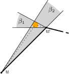
(b) Cones centered at $u$ and $w$

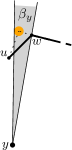
(c) Cone centered at $y$

Figure 7: Illustrations for the placement of the new bubbles $B_{e_{1}}$ and $B_{e_{2}}$

1. Bubble $B_{e_{1}}$ is located inside the empty neighborhood $\mathcal{N}$. Moreover, to preserve obtusity, $B_{e_{1}}$ needs to lie inside the semicircle with edge $e_{1}$ as diameter, as depicted in Figure 7a.

2. Consider angles $\beta_{1}$ and $\beta_{2}$ as illustrated in Figure 7b. We require that both angles are smaller than $\alpha/4$.

3. For any vertex $y$ of any extension of $\Gamma$, consider the angle $\beta_{y}$ as illustrated in Figure 7c. We require that this angle is smaller than $\alpha/4$. That guarantees that for any point $x\in B_{e_{1}}$ it holds that $\measuredangle(\overrightarrow{yw},\overrightarrow{yx})<\alpha/4$.

We define the bubble $B_{e_{2}}$ for the edge $e_{2}$ analogously with $B_{e_{1}}$. Moreover, we can use the same pair of parameters $r$ and $\varepsilon$ for $B_{e_{1}}$ and $B_{e_{2}}$.

For the strong monotonicity of the drawing $\Gamma$ with two new bubbles $B_{e_{1}}$ and $B_{e_{2}}$ we have to show two conditions: (1) that from any vertex stacked into one of the new bubbles there exists a strongly monotone path to any vertex $y$ of any extension of $\Gamma$ and (2) that there exists a strongly monotone path between any vertex stacked into $B_{e_{1}}$ and any vertex stacked into $B_{e_{2}}$.

Since we use the same pair of $r$ and $\varepsilon$ for defining $B_{e_{1}}$ and $B_{e_{2}}$, the condition (2) clearly holds as soon as $r/\varepsilon$ is small enough. Thus we are left with ensuring that the condition (1) holds.

Consider the new bubble $B_{e_{1}}$, a point $x\in B_{e_{1}}$ and any vertex $y$ of any extension $\Gamma^{\prime}$ of $\Gamma$. Since the drawing $\Gamma^{\prime}$ is strongly monotone, there exists a strongly monotone path $P_{yw}$ in $\Gamma^{\prime}$ between $y$ and $w$. Since $w$ has only two incident edges in $\Gamma^{\prime}$, the last edge of the path $P_{yw}$ is either $e_{1}=(u,w)$ or $e_{2}=(v,w)$. We distinguish between these two cases: in the first case we construct a path $P_{yx}$ from $y$ to $x$ by re-routing the last edge of $P_{yw}$ from $(u,w)$ to $(u,x)$ as illustrated in Figure 8a; in the second case we construct a path $P_{yx}$ by appending the edge $(w,x)$ to the end of $P_{yw}$ as illustrated in Figure 8b;

It remains to show that $P_{yx}$ is strongly monotone. First, observe that $P_{yw}$ is strongly monotone and $\alpha$-safe. By property (ii), the final edges $e_{w}$ of $P_{yw}$ and $e_{x}$ of $P_{yx}$ satisfy $\measuredangle(\overrightarrow{e_{w}},\overrightarrow{e_{x}})<\alpha/4$ and all other edges of these paths are identical. Thus, $P_{yx}$ is $(3\alpha/4)$-safe with respect to $\overrightarrow{yw}$. By Property (iii) $\measuredangle(\overrightarrow{yw},\overrightarrow{yx})<\alpha/4$ and, therefore, $P_{yx}$ is $(\alpha/2)$-safe with respect to $\overrightarrow{yx}$ and thus in particular it is strongly monotone.

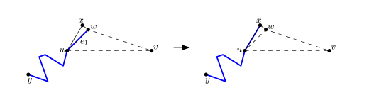
(a) Rerouting in case the last edge of $P_{yw}$ is $e_{1}$.

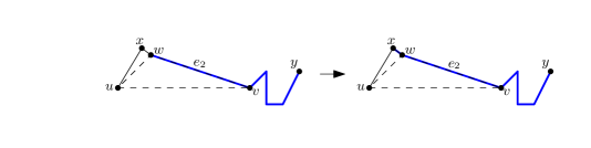
(b) Rerouting in case the last edge of $P_{yw}$ is $e_{2}$.

Figure 8: A strongly monotone path $P_{yw}$ from $y$ to $w$ is re-routed to $x$. Two possible cases are distinguished: The last edge of $P_{yw}$ is either $e_{1}$ or $e_{2}$.

The arguments for a vertex stacked on $e_{2}$ into $B_{e_{2}}$ are identical. ∎

Thus, we obtain the main result of this section:

Theorem 4.

Every 2-tree admits a strongly monotone drawing.

6 Conclusion

We have shown that any 3-connected planar graph, tree, outerplanar graph, and 2-tree admits a strongly monotone drawing. All our drawings require exponential area. For trees, this area bound has been proven to be required; however, it remains open whether the other graph classes can be drawn in polynomial area. Further, the question whether any 2-connected planar graph admits a strongly monotone drawing remains open. Last but not least, we could observe (using a computer-assisted search) that 2-connected graphs with at most 9 vertices admit a strongly monotone drawing, while there is exactly one connected graph with 7 vertices that is the smallest graph not admitting a strongly monotone drawing; see Figure 9.

Figure 9: The unique connected 7-vertex graph without a strongly monotone drawing.

References

- [1] Soroush Alamdari, Timothy M. Chan, Elyot Grant, Anna Lubiw, and Vinayak Pathak. Self-approaching graphs. In Walter Didimo and Maurizio Patrignani, editors, Proc. 20th Int. Symp. Graph Drawing (GD’12), volume 7704 of Lecture Notes Comput. Sci., pages 260–271. Springer, 2013.
- [2] Patrizio Angelini, Enrico Colasante, Giuseppe Di Battista, Fabrizio Frati, and Maurizio Patrignani. Monotone drawings of graphs. J. Graph Algorithms Appl., 16(1):5–35, 2012.
- [3] Patrizio Angelini, Walter Didimo, Stephen Kobourov, Tamara Mchedlidze, Vincenzo Roselli, Antonios Symvonis, and Stephen Wismath. Monotone drawings of graphs with fixed embedding. Algorithmica, 71:1–25, 2013.
- [4] Esther M. Arkin, Robert Connelly, and Joseph S. B. Mitchell. On monotone paths among obstacles with applications to planning assemblies. In Proc. 5th Ann. ACM Symp. Comput. Geom. (SoCG’89), pages 334–343. ACM, 1989.
- [5] Graham R. Brightwell and Edward R. Scheinerman. Representations of planar graphs. SIAM Journal on Discrete Mathematics, 6(2):214–229, 1993.
- [6] Hooman R. Dehkordi, Fabrizio Frati, and Joachim Gudmundsson. Increasing-chord graphs on point sets. In Christian Duncan and Antonios Symvonis, editors, Proc. 22nd Int. Symp. Graph Drawing (GD’14), volume 8871 of Lecture Notes Comput. Sci., pages 464–475. Springer, 2014.
- [7] Raghavan Dhandapani. Greedy drawings of triangulations. Discrete Comput. Geom., 43(2):375–392, 2010.
- [8] Stefan Felsner. Convex drawings of planar graphs and the order dimension of 3-polytopes. Order, 18(1):19–37, 2001.
- [9] Xin He and Dayu He. Compact monotone drawing of trees. In Dachuan Xu, Donglei Du, and Dingzhu Du, editors, Proc. 21st Int. Conf. Comput. Combin. (COCOON’15), volume 9198 of Lecture Notes Comput. Sci., pages 457–468. Springer, 2015.
- [10] Xin He and Dayu He. Monotone drawings of 3-connected plane graphs. In Nikhil Bansal and Irene Finocchi, editors, Proc. 23rd Ann. Europ. Symp. Algorithms (ESA’15), volume 9294 of Lecture Notes Comput. Sci., pages 729–741. Springer, 2015.
- [11] Md. Iqbal Hossain and Md. Saidur Rahman. Monotone grid drawings of planar graphs. In Jianer Chen, John E. Hopcroft, and Jianxin Wang, editors, Proc. 8th Int. Workshop Front. Algorithmics (FAW’14), volume 8497 of Lecture Notes Comput. Sci., pages 105–116. Springer, 2014.
- [12] Weidong Huang, Peter Eades, and Seok-Hee Hong. A graph reading behavior: Geodesic-path tendency. In Peter Eades, Thomas Ertl, and Han-Wei Shen, editors, Proc. 2nd IEEE Pacific Visualization Symposium (PacificVis’09), pages 137–144. IEEE Computer Society, 2009.
- [13] Christian Icking, Rolf Klein, and Elmar Langetepe. Self-approaching curves. Math. Proc. Camb. Philos. Soc., 125:441–453, 1995.
- [14] Philipp Kindermann, André Schulz, Joachim Spoerhase, and Alexander Wolff. On monotone drawings of trees. In Christian Duncan and Antonis Symvonis, editors, Proc. 22nd Int. Symp. Graph Drawing (GD’14), volume 8871 of Lecture Notes Comput. Sci., pages 488–500. Springer, 2014.
- [15] Bongshin Lee, Catherine Plaisant, Cynthia Sims Parr, Jean-Daniel Fekete, and Nathalie Henry. Task taxonomy for graph visualization. In Enrico Bertini, Catherine Plaisant, and Giuseppe Santucci, editors, Proc. AVI Workshop Beyond Time Errors: Novel Eval. Methods Inform. Vis. (BELIC’06), pages 1–5. ACM, 2006.
- [16] Tom Leighton and Ankur Moitra. Some results on greedy embeddings in metric spaces. Discrete Comput. Geom., 44(3):686–705, 2010.
- [17] Martin Nöllenburg and Roman Prutkin. Euclidean greedy drawings of trees. In Hans L. Bodlaender and Giuseppe F. Italiano, editors, Proc. 21st Europ. Symp. Algorithms (ESA’13), volume 8125 of Lecture Notes Comput. Sci., pages 767–778. Springer, 2013.
- [18] Martin Nöllenburg, Roman Prutkin, and Ignaz Rutter. On self-approaching and increasing-chord drawings of 3-connected planar graphs. arXiv:1409.0315, 2014.
- [19] Ananth Rao, Sylvia Ratnasamy, Christos H. Papadimitriou, Scott Shenker, and Ion Stoica. Geographic routing without location information. In David B. Johnson, Anthony D. Joseph, and Nitin H. Vaidya, editors, Proc. 9th Ann. Int. Conf. Mob. Comput. Netw. (MOBICOM’03), pages 96–108. ACM, 2003.
- [20] Kenneth Stephenson. Introduction to circle packing: the theory of discrete analytic functions. Cambridge Univ. Press, 2005.