Chemodynamic subpopulations of the Carina dwarf galaxy

Abstract

We study the chemodynamical properties of the Carina dwarf spheroidal by combining an intermediate spectroscopic resolution dataset of more than 900 red giant and red clump stars, with high-precision photometry to derive the atmospheric parameters, metallicities and age estimates for our targets. Within the red giant branch population, we find evidence for the presence of three distinct stellar sub-populations with different metallicities, spatial distributions, kinematics and ages. As in the Fornax and Sculptor dwarf spheroidals, the subpopulation with the lowest average metallicity is more extended and kinematically hotter than all other populations. However, we identify an inversion in the parallel ordering of metallicity, kinematics and characteristic length scale in the two most metal rich subpopulations, which therefore do not contribute to a global negative chemical gradient. Contrary to common trends in the chemical properties with radius, the metal richest population is more extended and mildly kinematically hotter than the main component of intermediate metallicity. More investigations are required to ascertain the nature of this inversion, but we comment on the mechanisms that might have caused it.

1 Introduction

Since the late 1970s, it has been suggested that the Milky Way’s halo has been assembled from the merging and accretion of many smaller systems (e.g. Searle & Zinn, 1978). In this paradigm, it has long been assumed that the Galaxy’s satellites are remnants of this population of building blocks. However, first analyses of the chemical abundances of the stellar populations in the surviving dwarf spheroidal galaxies (dSphs) appeared inconsistent with this idea (e.g., Shetrone et al., 2001; Venn et al., 2004). In particular, the metal-poor tail of the dSph metallicity distribution seemed significantly different from that of the Galactic halo (Helmi et al., 2006). Since then, extremely metal-poor stars have been discovered in Galactic satellite galaxies such as Sculptor (e.g.: Frebel et al., 2010a). Both the classical and the ultra-faint dSphs are now known to have a wide abundance dispersion and to host some of the most extreme metal-poor stars known. In fact, $\sim$ 30% of the known stars with [Fe/H] $\leq-3.5$ are found in dwarf galaxies (e.g. Kirby et al., 2010; Kirby & Cohen, 2012; Frebel et al., 2010b).

The connection between the surviving dwarfs and those that dissolved to form the halo can partially be addressed by examining in detail the stellar kinematics and chemical compositions of present-day dwarf galaxies. Establishing the detailed chemical histories of these systems can provide constraints on their dominant enrichment events and timescales. In addition, modelling of the kinematics can yield powerful information on the dark matter profile, especially in the case of multiple populations (e.g.: Walker & Peñarrubia, 2011; Amorisco & Evans, 2012a).

A multitude of independent studies have addressed the evolutionary complexities of dwarf spheroidal galaxies in the Local Group. Since Harbeck et al. (2001), stellar population gradients have been observed in many satellites of both the Milky Way and Andromeda – for example Sculptor (Tolstoy et al., 2004), Fornax (Battaglia et al., 2006), Sextans (Lee et al., 2003), Tucana (Harbeck et al., 2001), Draco (Faria et al., 2007), and And II (Ho et al., 2012). Whether such gradients are ubiquitous remains an open question, as dwarfs like Leo I, And I, And III and Carina seem to be characterised by more homogeneous stellar populations, with milder radial dependences (Harbeck et al., 2001; Koch et al., 2006, 2007).

A much closer look into specific dwarfs is allowed by large spectroscopic datasets. For example, in Sculptor, Fornax and Sextans, dedicated spectroscopic studies have allowed the identification of independent stellar subpopulations, with chemo-dynamically distinct properties (Battaglia et al., 2006; Battaglia et al., 2008, 2011; Walker & Peñarrubia, 2011; Amorisco & Evans, 2012b; Hendricks et al., 2014). By providing a bridge between chemical and kinematical properties of several hundreds of bright stars, chemo-dynamical analyses yield important constraints on the complex processes that govern the formation and evolution of such puny galaxies. For instance, subpopulations with a higher average metallicity are more centrally concentrated and kinematically colder. Whether the dwarf is characterised exclusively by old stellar populations – as in the case of Sculptor (see e.g. de Boer et al., 2012a) – or whether multiple populations of different ages are present at the same time – as in Fornax (e.g., de Boer et al., 2012b) – the parallel ordering of metallicity, characteristic scale of the stellar distribution and kinematical state seems to be a fundamental outcome of the dSphs’ evolutionary histories.

The importance of Carina is that it provides one of the cleanest examples of an episodic star formation (SF) history. This is evident from its colour-magnitude diagram (Tolstoy et al., 2009; Stetson et al., 2011), which clearly shows at least three different main sequence turn-offs. A number of investigations have inferred the SF history of Carina using photometric data (e.g., Hurley-Keller et al., 1998; Rizzi et al., 2003; Dolphin et al., 2005), with evidence for at least two major SF episodes, one at old times ($>8$ Gyr ago), a second at intermediate ages ($4-6\,{\rm Gyr}$ ago), and perhaps continuing into even more recent activity ($2\,{\rm Gyr}$ ago). Using both wide-field photometry and spectroscopic data, de Boer et al. (2014) find that about $60\%$ of the stars in Carina formed in the SF episode at intermediate ages. However, interestingly, as the oldest episode, also the intermediate one has enriched stars starting from low metallicities.

Given such a complex and episodic SF history, one would expect to detect similarly clear population gradients and chemo-dynamical differences in Carina’s stellar population. Based on deep multicolour photometry, Harbeck et al. (2001) find that red clump (RC) stars are indeed more concentrated than the older horizontal branch stars. However, no distinction in the spatial distribution of red and blue horizontal branch stars can be found (a gradient that is instead very clear in Sculptor, Tolstoy et al., 2004). More recently, Battaglia et al. (2012) observe an age gradient by selecting stellar populations of very different ages with cuts in the colour magnitude diagram (CMD). This confirms the existence of a marked age gradient over a baseline that is essentially as long as the age of the universe.

However, the presence of any gradient within the population of old red giant stars is substantially less clear, as is the existence of a corresponding metallicity gradient within the same population. By using a set of 437 radial velocity members, Koch et al. (2006) measure a very mild chemical gradient, with metal-poor stars having an only slightly more extended spatial distribution. Analogously, Walker & Peñarrubia (2011) could not identify any statistically significant distinction (in either spatial distribution or kinematics) by looking for two different subpopulations in a sample of more than 700 member red giants (RGs).

Because of their shallow potential wells, the evolutionary histories of dSphs are critically dependent on both properties before infall – for instance virial mass and gas content – and any subsequent environmental factors, mainly driven by the details of their orbits. In contrast to the wide orbits of Sculptor and Fornax, Carina’s proper motion (Piatek et al., 2003) suggests a pericenter of only a few tens of $\,{\rm kpc}$ from the centre of the Milky Way, which makes it more prone to tidal disturbances. Indeed, several investigations have identified a component of ‘extratidal’ stars around Carina (e.g., Majewski et al., 2005; Muñoz et al., 2006). Recent deep photometric studies (Battaglia et al., 2012) suggest the presence of tenuous but extended tails, and de Boer et al. (2014) has shown that these have compatible properties with Carina’s metal poor stars (although see also McMonigal et al., 2014). Interestingly, the perturbations arising from a tidal field have been shown to be capable of systematically weakening chemical gradients, by mixing any distinct stellar subpopulations (Sales et al., 2010; Pasetto et al., 2011).

In this paper, we present a new dataset that we use in order to bring further constraints on Carina’s history, based on intermediate resolution spectra of 956 stars. We describe how the analysis of the spectra has been done in order to derive the atmospheric parameters of the stars, namely the effective temperature (T_eff), surface gravity ($\log g$) and global metallicity ([M/H]), and how these parameters are combined with high precision photometry to derive an age estimate for the stars belonging to Carina. We find evidence for the presence of three distinct stellar subpopulations, and show the age-metallicity diagram of Carina. Finally we comment on the possible effects of external disturbances.

The paper is organised as follows: in Sect. 2 we describe the datasets used. Section 3 explains how the atmospheric parameters have been derived and the ages have been estimated. Finally, Sect. 4 shows the results and Sect. 5 concludes.

2 Presentation of the data

The available data include $1.3\times 10^{4}$ medium resolution spectra of 956 stars from the ESO-VLT large programmes, 180.B-0806, 084.B-0836 (P.I.: G. Gilmore) and our VISTA $JHK_{s}$ photometry. In addition, the photometric data is complemented by the high-precision optical $UBVRI$ photometry of Stetson et al. (2011).

The VLT datasets extend over 5 years, with some multiple observations of the same stars. The targets have been selected in order to sample the red clump and the giant branch of Carina, and have been observed using the LR8 setup of the FLAMES-GIRAFFE instrument ($820.6-940.0\,{\rm nm}$). For the spectra reduction and sky subtraction, we refer the reader to Koch et al. (2006), since the same method has been applied here too. The radial velocities have been estimated using the algorithm of Koposov et al. (2011), which delivers precise, accurate, radial velocities from moderate resolution spectroscopy. The algorithm works by fitting synthetic templates from Munari et al. (2005) covering a large range of stellar parameters ($-2.5<$[Fe/H] $<0.5$, 3000 $<$ T_eff$<$ 80000, 1.5 $<$ $\log g$$<$5) to our spectra from each exposure.

Once each exposure has been put in the rest frame, we have stacked the multiple exposures corresponding to each star in order to increase the signal-to-noise ratio (SNR) of the data. The final SNR spans values from 2 to 50 per pixel. Figure 1 shows the radial velocity distribution of the total sample of 956 stars observed with the LR8 setup. From this, we can see that most of the targeted stars peak at a common radial velocity, as expected. The Gaussian fit of the histogram has a mean radial velocity of $221.4\,{\rm km~{}s^{-1}}$ with a dispersion of $10\,{\rm km~{}s^{-1}}$, consistent with previous determinations of the radial velocity of Carina star members ranging from $220.4\,{\rm km~{}s^{-1}}$ to $224\,{\rm km~{}s^{-1}}$ and dispersions ranging from $6.8\,{\rm km~{}s^{-1}}$ to $11.7\,{\rm km~{}s^{-1}}$ (Mateo et al., 1998; Majewski et al., 2005; Helmi et al., 2006; Koch et al., 2006; Fabrizio et al., 2011; Lemasle et al., 2012).

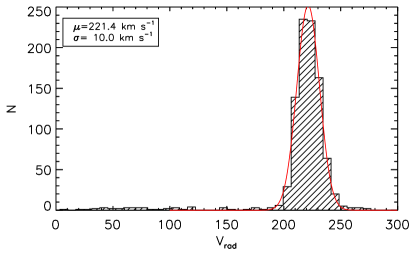
Figure 1: Histogram of the radial velocities for the total sample of stars observed at the LR8 setup (956 stars). The fitted Gaussian is plotted in red, and the fitting parameters are written on the top left corner of the figure. The mean value and dispersion of the radial velocity of Carina are in good agreement with the literature vaues.

3 Extraction of the atmospheric parameters and selection of the Carina subsample

Once the spectra are stacked, we used an updated version of the automatic parameterisation pipeline presented in Kordopatis et al. (2011a) to obtain the effective temperature, surface gravity and metallicity of the targets. The pipeline allows us to apply soft priors according to the observed selection function, by removing from the solution space combinations of parameters that are not expected to be found. The method is based on a grid of synthetic spectra used during the learning phase of the algorithm. Only the wavelength regions $840-877.5\,{\rm nm}$ and $880.1-882.0\,{\rm nm}$ are selected for the parameterisation, the discontinuity being introduced to avoid strong contamination by telluric lines and to keep within our wavelength range the MgI line at 8807Å, which is known to be sensitive to surface gravity variations (see Kordopatis et al., 2011b). Furthermore, the cores of the Calcium triplet lines are removed from the wavelength region (two pixels for the first line, and three for the other two lines, corresponding to 0.8 and 1.2Å, respectively), in order to avoid a mis-match between the synthetic spectra and the observations, due to non local thermodynamical equilibrium effects.

The learning grid has a constant metallicity step of $0.25\,{\rm dex}$, and spans effective temperatures from $[3000-8000]$ K, surface gravities from $[0-5]$($\,{\rm cgs}$ units) and metallicities from $[-5.0,+1.0]$. Finally, the $\alpha-$enhancement of the considered templates is not a free parameter, but it varies with metallicity ($[\alpha/$Fe$]=-0.4\times{\rm{[Fe/H]}}$ in the range $-1\leq{\rm{[Fe/H]}}\leq 0$). We note that this adopted $\alpha$-enhancement has no consequences for the determination of [M/H]  in the case where a star does not follow the same trend (as is expected to be the case for Carina dSph stars, see Venn et al., 2012). In such a case the measurement of [M/H]  will still be sound, but [M/H]$\neq$[Fe/H] (see Kordopatis et al., 2013, for further details).

We used the calibration relation established for RAVE DR4 (Kordopatis et al., 2013, see also Kordopatis et al. 2015), which employs the same grid of synthetic spectra on a very similar wavelength range, to correct the metallicities of the pipeline. The calibration is a simple low-order polynomial of two variables, the surface gravity and the metallicity itself, and roughly corrects the metallicity of the giants by $\sim 0.3\,{\rm dex}$ and the one of the dwarfs by $\sim 0.1\,{\rm dex}$. The adopted relation allowing to obtain the calibrated metallicity, [M/H]_c, from the one derived from the pipeline, [M/H]_p, is:

$$\begin{split}\hbox{[M/H]}_{c}-\hbox{[M/H]}_{p}=-0.076-0.006\times\log g+0.003\times\log^{2}g\\ -0.021\times\hbox{[M/H]}_{p}\times\log g+0.582\times\hbox{[M/H]}_{p}+0.205\times\hbox{[M/H]}_{p}^{2}.\end{split}$$ (1)

In what follows, only the corrected metallicities will be used, and therefore we will note the calibrated metallicities simply as [M/H].

As noted at the beginning of the Section, soft priors have been imposed on the expected results, by removing some parameter combinations from the solution space. For the adopted priors, we imposed:

• an effective temperature between $4000-6500$ K,

• a surface gravity lower than $3.75$,

• a metallicity range between $-5$ and $+1$ (i.e. all the available metallicity range of the templates).

The temperature range can be justified by the colour selection of Carina’s candidates ($0.5<B-V<1.2$, see Fig. 2). As fas as the assumption on the surface gravity is concerned, the reason relies on our a priori knowledge of the properties of the observed stars. Indeed, given the distance modulus of Carina ($m-M\sim 20.1$, e.g. Dall’Ora et al., 2003), all of Carina’s main sequence stars should be outside the observed magnitude range. In other words, all the stars belonging to Carina are expected to be either red clump stars or on the red giant branch, hence with a $\log g$ lower than 3.5.

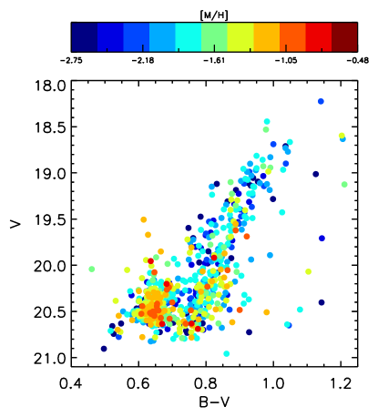
Figure 2: Colour-magnitude diagram of the final adopted Carina sample (731 members). The RC is at $(B-V)<0.7$ and $V>20$, whereas the RGB contains all the stars with $(B-V)>0.7$ up to $V=18$.

Figure 3: Histogram of the mean signal-to-noise ratio per pixel of the spectra of the final Carina sample that is considered for the analysis (731 members).

That said, one must still understand the effect of removing regions of the solution space on the parameterisation of foreground stars that might have the same radial velocity as Carina, and contaminate our sample (the risk here being to mis-parameterise a dwarf star as a giant). A first statement that can be made is that given the radial velocity of Carina ($221\,{\rm km~{}s^{-1}}$), foreground stars having a similar radial velocity are expected to be mainly halo stars, and therefore giants. For the few foreground stars that might still have $\log g$$>$3.75, the algorithm will always match, by design, the observations with the closest template (the latter being the one having the closest parameters as the true spectrum). This implies that the derived parameters of a dwarf star will therefore be at the boundaries of the grid and easily identifiable. In order to make sure that such contaminators are excluded from our analysis, we further decided to discard all the stars for which the surface gravity is greater than $3.25$, as well as the stars with a spectra having a SNR lower than 5 pixel^-1, because of the large uncertainty in the derived parameters. Figure 3 shows the SNR histogram of the Carina sample that is considered in what follows. The bulk of the spectra have SNR$\sim$10  pixel^-1, with some of them having up to SNR$\sim$40  pixel^-1. A selection of three spectra, at SNR$\sim 5,10,20$  pixel^-1, with their best-fit solution are shown in Fig. 4.

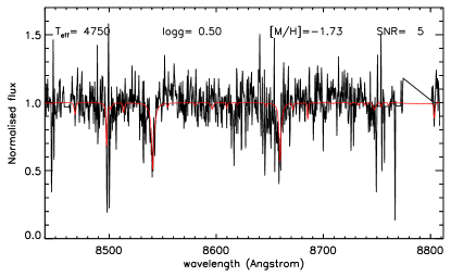
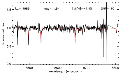
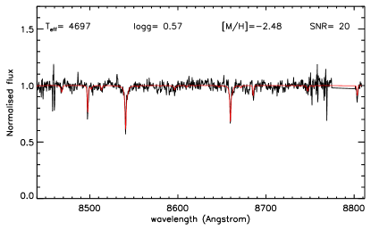
Figure 4: Observed (black) and fitted spectra (red) corresponding to the synthetic spectrum having the parameters of the stars for three stars having SNR$\sim 5,10,20$  pixel^-1. The wavelength range has been truncated at the blue end by $40$Å  to make the plots clearer to visualise.

Figure 5: Errors on the effective temperature, surface gravity, uncalibrated metallicity and calibrated metallicity as a function of signal-to-noise, for the sample of stars that we have identified as Carina members and with SNR greater than 5 pixel^-1.

Typical uncertainties on the parameters were obtained using the error spectrum of each target, producing 10 Monte-Carlo realisations of observed spectra and re-deriving the parameters. For T_eff, $\log g$ and [M/H], the median uncertainties are of the order of 226 K, 0.48 dex  and 0.29 dex, respectively, with the errors being the largest for the lowest SNR values, as expected (see Fig. 5).

Figure 2 shows the CMD for Carina for our adopted sample, colour-coded according to the metallicity of the stars. We find that the mean metallicity for the whole sample is $\hbox{[M/H]}\approx-1.78$, with a large span in the derived values, ranging from $\sim-4$ to $\sim-0.5$. This result is in very good agreement with previous studies (see for example Koch et al., 2006).

3.1 Age determination of the red giant branch stars

A rough estimate of the age of the stars can be obtained by comparing the colour, magnitudes and atmospheric parameters of the stars with theoretical isochrones. Following Kordopatis et al. (2011b), we constructed a library of isochrones with a constant step in age ($0.5\,{\rm Gyr}$) and metallicity ($0.1\,{\rm dex}$). The step in metallicity has been chosen in order to be smaller than the typical error on this parameter. The isochrones have been computed using the online interpolator of the Padova group, based on the Marigo et al. (2008) sets, for a metallicity range of $[-2.1;0.1]$. Since the isochrones do not reach as low metallicities as the metal-poorest stars in our sample, we do not attempt to derive ages for those stars that have a metallicity that does not reach $-2.1$ within $2\sigma_{\tiny\hbox{[M/H]}}$, where $\sigma_{\tiny\hbox{[M/H]}}$ is the uncertainty on the derived metallicity.

The expected age, $\bar{a}$, of a star with parameters $\hat{\theta}_{k}$ ($k\equiv\hbox{[M/H]}$, $V$, $B-V$, T_eff, $\log g$), has been obtained as follows. First, we select the set of isochrones within [M/H]$\pm\sigma_{\tiny\hbox{[M/H]}}$. Then, we assign for each point $i$ on the selected isochrones a Gaussian weight $W_{i}$ , which depends on the distance between the points on the isochrones and the measured observables or derived parameters. In practice, $W_{i}$ is computed as:

$$W_{i}=\mathrm{exp}\left(-\sum_{k}\frac{(\theta_{i,k}-\hat{\theta}_{k})^{2}}{2\sigma^{2}_{\hat{\theta}_{k}}}\right)$$ (2)

where $\theta_{i,k}$ corresponds to the considered parameters of the isochrones and $\sigma_{\hat{\theta}_{k}}$ to the associated uncertainties of the measurements. It is worth mentioning that we did not include to this weight any additional multiplicative factor proportional to the mass of the stars, as suggested by Zwitter et al. (2010, see also ) because this factor is useful only for surveys having a mixture of dwarfs and giants. Indeed, this factor defined as the stellar mass difference between two adjacent points on the isochrones, is introduced in order to give additional weight to the likelihood of observing a dwarf, because they are characterised by slower evolutionary phases. Since our survey includes only giant stars, this factor has been ignored.

The expected age $\bar{a}$ of a given star is then obtained by computing the weighted mean:

$$\bar{a}=\frac{\sum_{i}W_{i}\cdot a_{i}}{\sum_{i}W_{i}},$$ (3)

where $a_{i}$ are the associated ages of the points on the isochrones. The associated error of the expected age is obtained by:

$$\sigma(\bar{a})=\sqrt{\frac{\sum_{i}W_{i}\cdot[\bar{a}-a_{i}]^{2}}{\sum_{i}W_{i}}}.$$ (4)

We assumed a distance modulus for Carina of $m-M=20.1$ and a line-of-sight $E(B-V)=0.03$ mag, as estimated by, e.g. Dall’Ora et al. (2003) and Karczmarek et al. (2015). The considered age-range of the isochrones has been set to be between $1\,{\rm Gyr}$ and $13.7\,{\rm Gyr}$. We have tested two different configurations: one where only $V$, $(B-V)$ and the metallicity are taken into account, and one where we additionally consider the information related to the effective temperatures and surface gravities. Figure 6 shows the differences in the age estimations according to these two approaches for the RGB stars only (for the RC stars, see the discussion below). We can see that our sample can be separated at least into two populations, one old ($\sim 13\,{\rm Gyr}$), and one of intermediate age having a peak at $\sim 7.5\,{\rm Gyr}$ and with a much broader age range. This result is in good agreement with, for example Stetson et al. (2011), who fit the turn-off stars in the CMD and estimate that Carina has at least two populations: one of $12\,{\rm Gyr}$ and one of $4-6\,{\rm Gyr}$, or with Norris et al. (in prep) who are completing a similar age-metallicity analysis using high-resolution spectra of giant stars. In particular, we find that this intermediate age population has a tail extending to young ages, down to $1\,{\rm Gyr}$. Taking into account the atmospheric parameters in Eq. 2 does not change the age distributions drastically, as can be seen from the dotted (with T_eff, $\log g$) and plain (without T_eff, $\log g$) histograms of Fig. 6. This similarity in the age estimations shows that our effective temperatures, gravities and metallicities are consistent with the CMD of Carina. However, since the atmospheric parameters can have large covariances, and that the ages are not fundamentally changed when taking into account the T_eff and the $\log g$, in what follows, we have considered only the ages computed without taking into account the atmospheric parameters.

Figure 6: Age distribution of the RGB stars of Carina. The dotted (plain) line corresponds to age estimations with (without) taking into account the information on the effective temperature and gravity.

We note that for 10 stars, no age estimation was possible. The reason is that they are too far from the isochrones, either because they are foreground contaminators, binary stars, or stars for which the measurements (metallicity and/or photometry) are of poor quality and with underestimated errors.

3.2 Age determination of the red clump-region stars

The RC stars are massive stars which have passed through the explosive ignition of the Helium at the RGB tip and are now burning the helium core. Once all the helium in the core is exhausted, then the stars begin their AGB phase. Their absolute magnitude mildly depends on the metallicity and their age, with the oldest and most metal-poor ones being also the faintest.

The determination of the age of the stars in the RC region of the CMD ($B-V\leq 0.7$) by the projection on the isochrones is generally difficult to obtain because all the isochrones pass through that region. A first run of our pipeline on the stars in the RC-region has shown that the estimated ages of the bulk of these stars is similar to the intermediate age population of the RGB ($\sim 7.5\,{\rm Gyr}$ for the RGB, $\sim 6\,{\rm Gyr}$ for the RC-region), as expected from the observing biases (at these magnitudes, we do not see the oldest RC stars with still fainter magnitudes). Nevertheless, we find a non-negligible fraction of stars with ages lower than $4\,{\rm Gyr}$.

Since they do not have a counter-part (in terms of star-counts) on the RGB, it seems clear that the ages of the stars in the RC-region having low metallicities should have much older ages than what is derived (therefore likely being the oldest stars that have left the Horizontal Branch, and are now on the AGB. If these stars do follow the derived age-metallicity relation of the RGB stars, then their estimated ages should be $\sim 13\,{\rm Gyr}$. Given these facts we decide, in what follows, not to take into account the ages of the RC-region stars in our analysis.

4 Chemodynamical separation of the stellar populations

In order to identify and separate any chemodynamic stellar subpopulations, we use the maximum likelihood technique presented by Walker & Peñarrubia (2011) and later developed in Amorisco & Evans (2012b). We model the spectroscopic target as the combination of multiple subpopulations with different intrinsic properties, including metallicity, kinematics and spatial distribution. The crucial advances in this technique are that:

1. all available information can be used at the same time, improving the quality of the population division with respect to a method that only uses one dimension at a time (for example metallicity or kinematics, separately);

2. as a result of the population division, each single star is tagged with its membership probability to all identified subpopulations, so that with respect to the cross-contamination due to hard cuts, such a mixture model can better disentangle the properties of any different component;

3. the number of independent subpopulations needed to best describe the data can be determined objectively, by comparing the gain in likelihood due to the increased number of populations to the growth in the number of free parameters of the model;

4. any selection function can be explicitly taken into account.

Details on the technique can be found in Walker & Peñarrubia (2011) and Amorisco et al. (2014a). The mapping of the chemodynamical subpopulations onto the space of stellar ages is presented in Sect. 4.3.

Table 1: Three distinct chemo-dynamical subpopulations in the Carina dSph: the structural parameters.

Subpop	$\langle[{\rm M/H}]\rangle$	StD$([{\rm M/H}])$	$R_{\rm h}/$pc	$e$	$\langle\sigma_{LOS}\rangle/$kms-1	$f$
RGB Metal Poor (MP)	$-2.4\pm 0.1$	$0.21\pm 0.08$	$500^{+150}_{-75}$	$0.5\pm 0.15$	$10.4\pm 1$	$0.21\pm 0.06$
RGB Intermed. Met. (IM)	$-1.84\pm 0.05$	$0.10\pm 0.07$	$185\pm 20$	$\lesssim 0.2$	$7.6\pm 0.5$	$0.59\pm 0.04$
RGB Metal Rich (MR)	$-1.0\pm 0.1$	$0.23\pm 0.07$	$400^{+100}_{-50}$	$0.45^{+0.15}_{-0.1}$	$8.5\pm 0.8$	$0.20\pm 0.05$
Red Clump	$-1.50\pm 0.05$	$0.50\pm 0.05$	$225\pm 20$	$0.30\pm 0.06$	$8.6\pm 0.3$	–

4.1 Three distinct red giant branch subpopulations

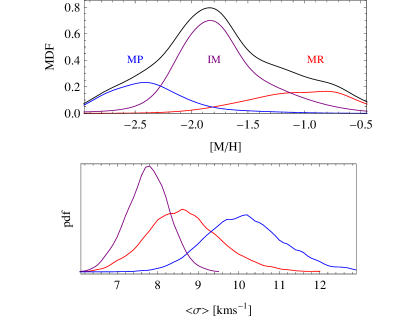
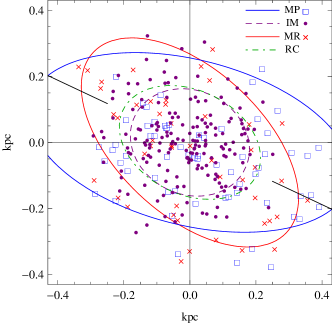
Figure 7: Three distinct subpopulations. Left upper panel: metallicity distribution function decomposed in three populations. Black: the MDF of the entire RGB sample. Blue, purple and red, respectively the contributions of metal-poor, intermediate-metallicity and metal-rich populations to the global RGB MDF. Note that distribution appear broader than the measured intrinsic spreads because of uncertainties on the discrete metallicity measurements. Left lower panel: the inference for the average velocity dispersion of the three RGB subpopulations. Right panel: the spatial distribution of the stars having more than 75 percent probability of being members (metal rich population in red, intermediate metallicity in purple, metal poor in blue). Coloured ellipses display the best fitting half-light radii for the each subpopulation; additionally the red clump population is in green and black lines display the position angle of the photometry and direction of Carina’s tidal tails.

We first restrict ourselves to the subset of high-probability Carina members belonging to the RGB ($B-V>0.7$, 400 members) and investigate any chemo-dynamical sub-divisions. We find that a two-populations model is preferred over one with a single population, but a model including three-populations represents the best description of the data (the probability of obtaining an analogous gain in the likelihood function by pure chance is negligible, despite the additional degrees of freedom of the three-populations model). Table 1 collects the properties of the three identified subpopulations.

We find that chemistry is the main driver of the division: we identify a metal poor (MP) population, with average metallicity of about $\langle[{\rm M/H}]\rangle\approx-2.4$, a population of intermediate metallicity (IM, $\langle[{\rm M/H}]\rangle\approx-1.8$) and a metal richer (MR) population, with $\langle[{\rm M/H}]\rangle\approx-1$. The upper-left panel in Fig. 7 displays the metallicity distribution function of our sample of red giant stars and illustrates the division in subpopulations. The bulk of Carina’s red giants belong to the population of intermediate metallicity, collecting a fraction $f_{\rm IM}\approx 60\%$ of the total RGB population, similarly to what found by de Boer et al. (2014). Note that this plot includes both (i) a convolution with the individual observational uncertainty of each metallicity measurement and (ii) the partial weighing of each star with its membership probability to each subpopulation. The first is responsible for the larger metallicity spread of each population (with respect to the intrinsic spread listed in Table 1), while the second is responsible for the skewness and overlap between the different populations due to those stars that have similar probabilities of belonging to either population (caused by both observational uncertainties in metallicity and by the similarity between the recovered kinematical properties of the populations).

The right panel of Fig. 7 shows the spatial distribution of the three subpopulations, with symbols identifying the high probability members ($p\geq 0.75$). Each ellipse corresponds to the best fitting elliptical half-light radius $R_{\rm h}$, with its ellipticity and position angle. The properties of the spatial distributions of the different populations are obtained by assuming a parametric functional form (Plummer profile) and by fitting for the spatial distribution of discrete spectroscopic targets, following Walker & Peñarrubia (2011), but also allowing for a non zero ellipticity.

The MP population is considerably elongated and extended. In fact, we are not entirely able to measure its half-light radius, as we find that its distribution in the radial range probed by our data is almost flat. We find that MP stars are approximately aligned with Carina’s tidal tails, as measured by Battaglia et al. (2012). The MR population is somewhat less extended, although also quite spread out over our radial coverage. On the contrary, the IM population is substantially more compact and centrally peaked, with a well defined half-light radius and a decreasing number counts profile.

In contrast with all other previously studied dSphs, we find that the MR population is more extended than the IM population, and, accordingly, its characteristic velocity dispersion is most likely larger, as shown in the lower-left panel of Fig. 7. This inversion can be captured even with hard cuts in metallicity, i.e. without the use of the likelihood division method. Although such a binning makes the signal weaker due to the large errors in metallicities, the trends shown in Fig. 8 indicate, indeed, that the high metallicity tail is at least as kinematically hot than the bulk of the stars in the intermediate-metallicity bin. The same cuts can be used to show that the spatial distribution of the stars in the intermediate-metallicity bin is more compact than that of the high-metallicity tail, proving that our result is robust.

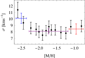
Figure 8: Projected velocity dispersion versus metallicity, obtained by simply binning the spectroscopic data for the RGBs. Black points are obtained using subsets of 50 RGBs each (successive bins shift by 25 stars at a time, so that not all data points are independent). All measurements are obtained through a maximum likelihood method, and the vertical error bars show $1\sigma$ uncertainties. The wider and coloured error bars group RGB stars into wider bins, and are fully independent from each other (respectively, the three bins contain 75, 250, 75 RGBs).

This represents the first case in which it is not possible to identify a complete parallel ordering of metallicity, characteristic scale of the stellar distribution and kinematical state. The MR population is more extended than the IM population, and, at the same time, at least as kinematically hot. In turn, this may provide a justifications to previous measurements of a very limited global chemical gradient in both Koch et al. (2006) and Walker & Peñarrubia (2011).

4.2 Comparison with the Red Clump population

We have decided to carry out a separate analysis of the RC population, keeping it distinct from the RGB population. We do not try to separate subpopulations based on chemistry within the RC, and instead only measure global properties of their spatial distribution, kinematics and chemistry.

We use more than 400 line-of-sight velocity measurements and associated spatial position for RC stars that belong to Carina with high probability. As listed in Table 1, we find that the RC population bears significant similarities with the population of intermediate metallicity in the red giant branch. Its half light radius is comparable with the half light radius of the photometry and so are its ellipticity and position angle (as shown in the right panel of Fig. 7). Note that, being on average slightly younger, it is likely that the RC population probes a combination of the IM and MR red giant subpopulations. Therefore, the fact that the IM population is even more concentrated than the RC population is a confirmation of the inversion described in the previous section. The same reasoning applies to the kinematics of the RC population, whose velocity dispersion is slightly hotter than the the one of the IM population.

4.3 Age decomposition of the red giant branch stars

In this section, we investigate how the chemo-dynamical population splitting we have just obtained projects into the space of stellar ages. Grey points in Fig. 9 illustrate the age-metallicity relation for the RGB stars we have derived and presented in Sect. 3.1 (error-bars are also shown for a selection of precise measurements, where uncertainties are lower than $1.5\,{\rm Gyr}$). As previously noted, despite Carina’s narrow RGB and the well known age-metallicity degeneracy which makes the uncertainty on the age of any single RG substantial, we identify a well defined age-metallicity relation on the whole population, thanks to the precise photometry of Stetson et al. (2011) and metallicity estimates of our analysis.

High-probability members of each subpopulation are highlighted in different colours in the lower panel of Fig. 9. They do not clearly separate out in age, but the presence of a gradient in the mean ages of the three populations is clear. The upper panel of Fig. 9 directly projects the population split into the space of stellar ages, by showing the distributions of the ages of members of each stellar subpopulation (as for plots in Fig. 7, distributions in Fig. 9 are convolved with the uncertainties of each single age measurement, which contribute to broaden each probability distribution substantially). We find that the MP stellar population almost exclusively contains stars that are associated with the oldest isochrone in our library ($13.7\,{\rm Gyr}$), the IM has a considerable component of intermediate age stars ($6-10\,{\rm Gyr}$), while, to continue the gradient, the MR population extends up to recent times.

Even though the task of individual age estimation remains challenging, we find that the chemodynamical division into subpopulations of the Carina dSph is globally compatible with the independent picture presented by its SF history. As the photometrically derived SF history suggests, Carina has experienced three major SF episodes. Indeed, we find independent and corroboratory evidence for this in the spectroscopy: three stellar subpopulations are identified, with ages compatible with those indicated by the SF history.

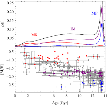
Figure 9: Subpopulations and ages. Upper panel: the probability distribution for the age of the three distinct chemo-dynamical subpopulations in Carina (metal rich in red, intermediate in purple, metal poor in blue, total in black). Lower panel: the age-metallicity diagram for the RGB stars in the spectroscopic sample; error bars are shown only for stars with a precise age estimate ($\delta_{\rm age}\leq 1.5$ Gyr); colored points identify high-probability members (probability of being a member larger than 75 percent) for each chemo-dynamical subpopulation.

5 Discussion and Conclusions

We have shown that, similar to Fornax and Sculptor, the Carina dSph is characterised by the presence of multiple stellar populations, with distinct chemical properties, spatial distributions and kinematical states. However, Carina appears substantially more mixed than either Sculptor or Fornax, which is reflected in the comparatively smaller differences among the characteristic scale lengths (as well as velocity dispersions) of its subpopulations. The MP population is more extended (and kinematically hotter) than the two younger populations (respectively IM and MR). What is more notable is that we find that the youngest MR population is more extended and at least as kinematically hot as the IM population, with evidence for an inversion of the usual ordering. Accordingly, the IM metallicity population is also more concentrated than the RC population.

While metal richer stellar subpopulations are generally more spatially concentrated and accordingly kinematically colder, the evolutionary history of Carina partially broke this common parallel ordering. This opens the question as to whether Carina’s stellar populations were formed with the properties we observe today – and then any difference from Fornax or Sculptor has to be found in the intrinsic properties and triggers of the SF episodes – or whether Carina initially had a more pronounced chemical gradient but this was subsequently perturbed by environmental factors.

Sales et al. (2010) have shown that strong enough tidal disturbances may be capable of homogenising the properties of multiple subpopulations. They suggest that, by removing a substantial fraction of the outer dark matter envelope, stripping causes the velocity dispersion of extended populations to decrease, weakening any kinematical difference with more concentrated tracers. Indeed, Carina’s proper motion suggests a pericenter of only a few tens of  kpc, which is considerably smaller than either Fornax or Sculptor. Also, the presence of an extended extratidal component would suggest tidal disturbance as a feasible mechanism to mix the originally more segregated subpopulations of Carina after infall.

However, it remains unclear whether tides alone can be responsible for Carina’s present configuration. In particular, tidal effects are strongest on more extended populations which implies that they should naturally preserve any original outside-in ordering in the characteristic scales of stellar subpopulations: it seems somewhat puzzling that tides are capable of causing an inversion in the ordering of the subpopulations as observed here. As a consequence, it is tempting to discuss other possible mechanism that may cause such phenomenology.

If the current distribution of the MR population has not been altered by tides, then the gas from which it is was originated was initially more spread out than the gas from which the IM population was born. In the following we list mechanisms that may be held responsible for this.

• Ram pressure: if the MR is formed after infall, gas may have been disturbed by the interaction with the corona of the Milky Way, in the form of ram pressure, perhaps also triggering star formation (see also Nayakshin & Wilkinson, 2013, on how Milky Way feedback can affect the evolution of dSph satellites, even at $100\,{\rm kpc}$).

• Stellar feedback from the IM population: if not energetic enough to entirely remove the remaining gas, feedback would naturally result in the gas being distributed on more energetic orbits (an illustration of this effect has been recently provided by El-Badry et al., 2015). It is unclear however if the cooling necessary to restart star formation would newly concentrate it in the central regions.

• Interaction with an another dwarf galaxy or dark halo, likely before infall, that may have triggered the star formation and perturbed the gas by dynamical interaction.

D’Onghia & Lake (2008) have suggested low mass galaxies only light up with star formation when belonging to groups at intermediate redshifts. Indeed, star formation is quite challenging to achieve in such small haloes (e.g., Read et al., 2006) and the larger virial mass of a group may help dwarfs to more easily retain their gas after episodes of intense stellar feedback (e.g., Peñarrubia et al., 2012; Amorisco et al., 2014b). Here we note that interactions between low mass dwarfs may also contribute in triggering and facilitating star formation, in a systematic way over the population of low mass galaxies. Such interactions are not unfrequent in a $\Lambda$CDM universe (e.g., Deason et al., 2014; Wetzel et al., 2015), and would justify the fact that a fraction of the low mass members of the Local Group show signs suggesting a violent and active past (Kleyna et al., 2003; Coleman et al., 2004; Amorisco et al., 2014a; de Boer et al., 2014).

References

- Amorisco & Evans (2012a) Amorisco N. C., Evans N. W., 2012a, MNRAS, 419, 184
- Amorisco & Evans (2012b) Amorisco N. C., Evans N. W., 2012b, ApJ, 756, L2
- Amorisco et al. (2014a) Amorisco N. C., Evans N. W., van de Ven G., 2014a, Nature, 507, 335
- Amorisco et al. (2014b) Amorisco N. C., Zavala J., de Boer T. J. L., 2014b, ApJ, 782, L39
- Battaglia et al. (2006) Battaglia G., et al., 2006, A&A, 459, 423
- Battaglia et al. (2008) Battaglia G., Helmi A., Tolstoy E., Irwin M., Hill V., Jablonka P., 2008, ApJ, 681, L13
- Battaglia et al. (2011) Battaglia G., Tolstoy E., Helmi A., Irwin M., Parisi P., Hill V., Jablonka P., 2011, MNRAS, 411, 1013
- Battaglia et al. (2012) Battaglia G., Irwin M., Tolstoy E., de Boer T., Mateo M., 2012, ApJ, 761, L31
- Coleman et al. (2004) Coleman M., Da Costa G. S., Bland-Hawthorn J., Martínez-Delgado D., Freeman K. C., Malin D., 2004, AJ, 127, 832
- D’Onghia & Lake (2008) D’Onghia E., Lake G., 2008, ApJ, 686, L61
- Dall’Ora et al. (2003) Dall’Ora M., et al., 2003, AJ, 126, 197
- Deason et al. (2014) Deason A., Wetzel A., Garrison-Kimmel S., 2014, ApJ, 794, 115
- Dolphin et al. (2005) Dolphin A. E., Weisz D. R., Skillman E. D., Holtzman J. A., 2005, ArXiv Astrophysics e-prints,
- El-Badry et al. (2015) El-Badry K., Wetzel A. R., Geha M., Hopkins P. F., Kereš D., Chan T. K., Faucher-Giguère C.-A., 2015, preprint, (arXiv:1512.01235)
- Fabrizio et al. (2011) Fabrizio M., et al., 2011, PASP, 123, 384
- Faria et al. (2007) Faria D., Feltzing S., Lundström I., Gilmore G., Wahlgren G. M., Ardeberg A., Linde P., 2007, A&A, 465, 357
- Frebel et al. (2010a) Frebel A., Kirby E. N., Simon J. D., 2010a, Nature, 464, 72
- Frebel et al. (2010b) Frebel A., Simon J. D., Geha M., Willman B., 2010b, ApJ, 708, 560
- Harbeck et al. (2001) Harbeck D., et al., 2001, AJ, 122, 3092
- Helmi et al. (2006) Helmi A., et al., 2006, ApJ, 651, L121
- Hendricks et al. (2014) Hendricks B., Koch A., Walker M., Johnson C. I., Peñarrubia J., Gilmore G., 2014, A&A, 572, A82
- Ho et al. (2012) Ho N., et al., 2012, ApJ, 758, 124
- Hurley-Keller et al. (1998) Hurley-Keller D., Mateo M., Nemec J., 1998, AJ, 115, 1840
- Karczmarek et al. (2015) Karczmarek P., et al., 2015, AJ, 150, 90
- Kirby & Cohen (2012) Kirby E. N., Cohen J. G., 2012, AJ, 144, 168
- Kirby et al. (2010) Kirby E. N., et al., 2010, ApJS, 191, 352
- Kleyna et al. (2003) Kleyna J. T., Wilkinson M. I., Gilmore G., Evans N. W., 2003, ApJ, 588, L21
- Koch et al. (2006) Koch A., Grebel E. K., Wyse R. F. G., Kleyna J. T., Wilkinson M. I., Harbeck D. R., Gilmore G. F., Evans N. W., 2006, AJ, 131, 895
- Koch et al. (2007) Koch A., Wilkinson M. I., Kleyna J. T., Gilmore G. F., Grebel E. K., Mackey A. D., Evans N. W., Wyse R. F. G., 2007, ApJ, 657, 241
- Koposov et al. (2011) Koposov S. E., et al., 2011, ApJ, 736, 146
- Kordopatis et al. (2011a) Kordopatis G., Recio-Blanco A., de Laverny P., Bijaoui A., Hill V., Gilmore G., Wyse R. F. G., Ordenovic C., 2011a, A&A, 535, A106
- Kordopatis et al. (2011b) Kordopatis G., et al., 2011b, A&A, 535, A107
- Kordopatis et al. (2013) Kordopatis G., et al., 2013, AJ, 146, 134
- Kordopatis et al. (2015) Kordopatis G., et al., 2015, MNRAS, 447, 3526
- Lee et al. (2003) Lee M. G., et al., 2003, AJ, 126, 2840
- Lemasle et al. (2012) Lemasle B., et al., 2012, A&A, 538, A100
- Majewski et al. (2005) Majewski S. R., et al., 2005, AJ, 130, 2677
- Marigo et al. (2008) Marigo P., Girardi L., Bressan A., Groenewegen M. A. T., Silva L., Granato G. L., 2008, A&A, 482, 883
- Mateo et al. (1998) Mateo M., Hurley-Keller D., Nemec J., 1998, AJ, 115, 1856
- McMonigal et al. (2014) McMonigal B., et al., 2014, MNRAS, 444, 3139
- Muñoz et al. (2006) Muñoz R. R., et al., 2006, ApJ, 649, 201
- Munari et al. (2005) Munari U., Sordo R., Castelli F., Zwitter T., 2005, A&A, 442, 1127
- Nayakshin & Wilkinson (2013) Nayakshin S., Wilkinson M. I., 2013, MNRAS, 433, 324
- Pasetto et al. (2011) Pasetto S., Grebel E. K., Berczik P., Chiosi C., Spurzem R., 2011, A&A, 525, A99
- Peñarrubia et al. (2012) Peñarrubia J., Pontzen A., Walker M. G., Koposov S. E., 2012, ApJ, 759, L42
- Piatek et al. (2003) Piatek S., Pryor C., Olszewski E. W., Harris H. C., Mateo M., Minniti D., Tinney C. G., 2003, AJ, 126, 2346
- Read et al. (2006) Read J. I., Pontzen A. P., Viel M., 2006, MNRAS, 371, 885
- Rizzi et al. (2003) Rizzi L., Held E. V., Bertelli G., Saviane I., 2003, ApJ, 589, L85
- Sales et al. (2010) Sales L. V., Helmi A., Battaglia G., 2010, Advances in Astronomy, 2010, 18
- Searle & Zinn (1978) Searle L., Zinn R., 1978, ApJ, 225, 357
- Shetrone et al. (2001) Shetrone M. D., Côté P., Sargent W. L. W., 2001, ApJ, 548, 592
- Stetson et al. (2011) Stetson P. B., et al., 2011, The Messenger, 144, 32
- Tolstoy et al. (2004) Tolstoy E., et al., 2004, ApJ, 617, L119
- Tolstoy et al. (2009) Tolstoy E., Hill V., Tosi M., 2009, ARA&A, 47, 371
- VandenBerg et al. (2015) VandenBerg D. A., Stetson P. B., Brown T. M., 2015, ApJ, 805, 103
- Venn et al. (2004) Venn K. A., Irwin M., Shetrone M. D., Tout C. A., Hill V., Tolstoy E., 2004, AJ, 128, 1177
- Venn et al. (2012) Venn K. A., et al., 2012, ApJ, 751, 102
- Walker & Peñarrubia (2011) Walker M. G., Peñarrubia J., 2011, ApJ, 742, 20
- Wetzel et al. (2015) Wetzel A. R., Deason A. J., Garrison-Kimmel S., 2015, ApJ, 807, 49
- Zwitter et al. (2010) Zwitter T., et al., 2010, A&A, 522, A54
- de Boer et al. (2012a) de Boer T. J. L., et al., 2012a, A&A, 539, A103
- de Boer et al. (2012b) de Boer T. J. L., et al., 2012b, A&A, 544, A73
- de Boer et al. (2014) de Boer T. J. L., Tolstoy E., Lemasle B., Saha A., Olszewski E. W., Mateo M., Irwin M. J., Battaglia G., 2014, A&A, 572, A10