Sulphur abundance determinations in star-forming regions-I: Ionization Correction Factor

Abstract

In the present work we used a grid of photoionization models combined with stellar population synthesis models to derive reliable Ionization Correction Factors (ICFs) for the sulphur in star-forming regions. These models cover a large range of nebular parameters and yielding ionic abundances in consonance with those derived through optical and infrared observational data of star-forming regions. From our theoretical ICFs, we suggested an $\alpha$ value of $3.27\pm 0.01$ in the classical Stasińska formulae. We compared the total sulphur abundance in the gas phase of a large sample of objects by using our Theoretical ICF and other approaches. In average, the differences between the determinations via the use of the different ICFs considered are similar to the uncertainties in the S/H estimations. Nevertheless, we noted that for some objects it could reach up to about 0.3 dex for the low metallicity regime. Despite of the large scatter of the points, we found a trend of S/O ratio to decrease with the metallicity, independently of the ICF used to compute the sulphur total abundance.

1 Introduction

The knowledge of the abundance of heavy elements (e.g. O, S, N, Ne) in the gas phase of star-forming regions play a key role in studies of stellar nucleosynthesis, initial mass function of stars and chemical evolution of galaxies.

To derive the total abundance of a given element (X) in ionized nebulae, after to estimate the electron temperature and electron density of the gas phase, it is necessary to calculate the abundance of all its ionization stages (see Osterbrock 1989). However, for the majority of the elements present in star-forming regions, only emission-lines of some ionization stages can be measured. In these cases, the use of Ionization Correction Factors (ICFs) is necessary to derive the contribution of unobserved ions, as initially defined by Peimbert & Costero (1969)

$$\rm ICF(X^{+i})=\frac{X/H}{X^{+i}/H^{+}},$$ (1)

where $\rm X^{+i}$ is the ion whose ionic abundance can be calculated from its observed emission-lines.

In particular, for sulphur, in the most of the cases the total abundance is calculated by a direct determination of the abundance of the ions $\rm S^{+}$ and $\rm S^{2+}$, through the lines [S ii]$\lambda$$\lambda$6716,31 and [S iii]$\lambda$$\lambda$9069, 9532 respectively, and by using an ICF to correct the unobserved $\rm S^{3+}$, which produces forbidden lines at 10.51$\mu$m. In the pioneer work, Stasińska (1978a) proposed an ICF for the sulphur based on both $\rm S^{+}$ and $\rm S^{2+}$ ions and given by

$$\rm ICF(S^{+}+S^{2+})=\left[1-\left(1-\frac{O^{+}}{O}\right)^{\alpha}\right]^{-1/\alpha}.$$ (2)

Along decades, the value of $\alpha$ have been largely discussed in the literature. For example, Stasińska (1978a), using the photoionization models of Stasińska (1978b), which assume the Non Local Thermodynamic Equilibrium (NLTE) stellar atmosphere models of Mihalas (1972), suggested $\alpha=3$. French (1981), who used a sample of H ii regions and planetary nebulae, derived $\alpha=2$. Garnett (1989) combined spectroscopic data of H ii regions containing the [S iii]$\lambda$$\lambda$9069, 9532 emission-lines (not considered by most of previous works) with photoionization models assuming different stellar atmosphere models in order to estimate an ICF for the sulphur. From this analysis, Garnett (1989) suggested that an intermediary $\alpha$ value between 2 and 3 is correct. Vermeij & van der Hulst (2002), using the optical and infrared spectroscopic data of Vermeij et al. (2002), were able to derive directly an ICF for the sulphur and concluded that $\alpha=3$ is correct for $\rm O^{+}/O\>>0.2$, being their results less clear for higher ionization stages (see also Dennefeld & Stasińska 1983; Izotov et al. 1994; Thuan et al. 1995; Kwitter & Henry 2001; Kennicutt et al. 2003; Pérez-Montero et al. 2006). Direct estimations for the sulphur ICF, such as the one performed by Vermeij & van der Hulst (2002), require infrared spectroscopic data of H ii regions as well as direct measures of electron temperatures, difficult for objects with low ionization degrees (Bresolin et al., 2005). Thus, sulphur ICFs have been mainly calculated by using photoionization models, in which not comparison with observational data are performed.

Other important subject is the relative abundance between sulphur and oxygen, which has a direct impact on studies of stellar nucleosynthesis. These elements arise from the nucleosynthesis in massive stars (Arnett, 1978; Woosley & Weaver, 1995), however, there are two fundamental issues ill-defined: (a) The knowledge of the mass range of stars that dominates the production of these elements. (b) If the initial mass function (IMF) of stars is universal. For decades, studies based on optical spectroscopic data of star-forming regions have been used to solve these problems but, not conclusive results were obtained. For example, Garnett (1989), who derived sulphur abundances for a sample of 13 extragalactic H ii regions, found a constant S/O abundance over a range of O/H (generally used as metallicity tracer), which suggests that either these elements are produced by massive stars within a similar mass range or by stars of different masses but with an universal IMF (Henry & Worthey, 1999). This result is supported by the majority of other works done in this direction (e.g. Berg et al. 2013; Guseva et al. 2011; Pérez-Montero et al. 2006; Kennicutt et al. 2003). However, evidences of S/O ranges with O/H were found, for example, by Vílchez et al. (1988) in the galaxy M 33 and by Díaz et al. (1991) in M 51. Moreover, due to large dispersion in S/O for a fixed value of O/H (see e.g. Hägele et al., 2012, 2008, 2006), the idea that S/O does not range with the metallicity is somewhat uncertain (Pérez-Montero et al., 2006; Kehrig et al., 2006).

In this paper, we employ a grid of photoionization models of H ii regions and a large sample of optical and infrared spectroscopic data of star-forming regions with the following goals:

1. To derive ICFs for the sulphur based on a consistent comparison between ionic abundances predicted by photoionization model and calculated from observational data.

2. To compare the discrepancy in S/H abundances computed by using different ICFs.

3. To investigate the S/O-O/H relation in star-forming regions considering different ICFs for the sulphur.

This paper is the first (Paper I) of a series of three works, where in the out-coming papers we will present a comparison of $\rm S^{2+}/H^{+}$ abundances obtained from optical and infrared lines and a comparison between S/O and O/H abundances with prediction of chemical evolution models. Similar analysis was performed for the neon by Dors et al. (2013). The present paper is organized as follows. In Section 2 the observational data used along the paper are presented. In Section 3, we describe the photoionization models used to derive ICFs for the sulphur, while methodology adopted to derive the ionic abundances is given in Section 4. In Section 5 the results containing the ICFs obtained by using photoionization models and from observational emission-lines are presented. Discussion and conclusions regarding the outcome are given in Sections 6 and 7, respectively.

2 Observational data

We compiled from the literature emission-line intensities of H ii regions and star-forming galaxies obtained in the optical and infrared spectral ranges. These measurements were used to obtain sulphur and oxygen ionic abundances in order to verify if our photoionization models are representative of real H ii regions, to check if the theoretical ICFs are compatible with the ones derived directly from observations and investigating the S/O-O/H relation. The selection criterion for the Visible-sample was the detection of the intensity lines [O ii]$\lambda$$\lambda$3726+ 29 (hereafter refereed as [O ii]$\lambda$3727), [O iii]$\lambda$$\lambda$4363, 5007, [S ii]$\lambda$$\lambda$6717, 31 and [S iii]$\lambda$9069. In the cases where the [S ii]$\lambda$6717 and $\lambda$6731 lines were not resolved, the sum of the intensity of these lines were considered. For some objects (indicated in Table 5) the theoretical relation $I$[S iii]$\lambda$9069=$I$[S iii]$\lambda$9532/2.5 was used to estimate the emission line intensity of $\lambda$9069, since only the sum of these was available.

Since H ii regions and star-forming galaxies are indistinguishable in diagnostic diagrams (e.g. Dors et al. 2013), these objects were considered jointly in our analysis. To eliminate objects with a secondary ionizing source, we use the criterion proposed by Kewley et al. (2001) to distinguish objects ionized by massive stars from those containing an active galactic nucleus (AGN) and/or gas shock. Hence all objects with

$$\rm log[O\>III]\lambda 5007/H\beta\><\>\frac{0.72}{[log([S\>II]\lambda\lambda 6717+31/H\alpha)]-0.32}$$ (3)

were selected. In Figure 1 the objects in our sample and a curve representing the criterion above are shown.

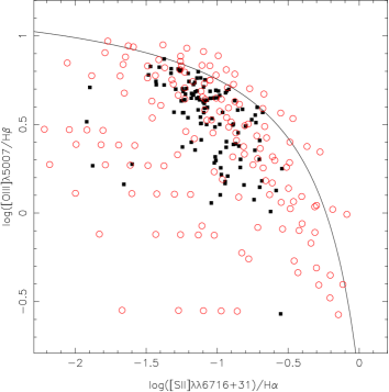
Figure 1: $\rm log[O\>III]\lambda 5007/H\beta$ vs. $\rm log([S\>II]\lambda\lambda 6717+31/H\alpha)$ diagnostic diagram. Solid line, taken from Kewley et al. (2001), separates objects ionized by massive stars from those containing active nuclei and/or shock-excited gas. Black squares represent the objects in our sample. Open circles represent estimations predicted by our models (see Sect. 3).

In the Appendix, Table 5 lists the object identification, optical emission-line intensities (relative to H$\beta$=100) and bibliographic references of the sample. We obtained optical data of 118 objects. All emission-line intensities were reddening corrected by the authors of the original works from which we have taken the data. Dors et al. (2013) showed that effects of using heterogeneous data sample, such as the one used in this paper, do not yield any bias on the results of abundance estimations in the gas phase of star-forming regions.

We also considered emission-line intensities of 143 H ii galaxies of a sample of 310 galaxies considered by Izotov et al. (2006a) and selected from the Sloan Digital Sky Survey (York et al., 2000) Data Release 3 . We applied a similar selection criterion above but with small changes due to the shorter wavelength spectral coverage of the Sloan data (when [O ii]$\lambda$3727 is observed [S iii]$\lambda$9069 is not, and vice versa, depending on the object redshift). Hence we selected the objects that present the [S iii]$\lambda$9069 emission lines and [O ii]$\lambda$7325 instead of [O ii]$\lambda$3727. These objects are also represented in Fig. 1 but are not listed in Table 5.

Concerning the IR-sample, the selection criterion was the presence of the flux measurements of the emission-lines H i 4.05 $\mu$m, [S iv] 10.51$\mu$m and [S iii]18.71$\mu$m. We compiled infrared data of 103 objects classified as being H ii regions and nuclei of galaxies containing star-formation regions. Only nine objects have both optical and IR data. In the Appendix, in Table 6, object identification, fluxes of the emission-lines considered and bibliographic references of the sample are listed. In some cases, indicated in Table 6, the H i 4.05 $\mu$m emission-line fluxes were computed from H i 12.37 $\mu$m or H I 2.63 $\mu$m fluxes, assuming the theoretical ratios H i 4.051$\mu$m/H i 12.37$\mu$m=8.2 and H I 4.051$\mu$m/H I 2.63$\mu$m=1.74 taken from Storey & Hummer (1995) for $N_{\rm e}=100$ cm^-3 and $T_{\rm e}=10\>000$ K.

For the objects with emission-line measurements at different spatial positions, indicated in the Table 6, the adopted fluxes were the sum (integrated) of the individual ones. The purpose of this procedure is to avoid taking exclusive emission-lines from outer parts of H ii regions into account, which the diffuse gas emission (e.g. Helmbold et al. 2005; Walterbos 1998) component can be important but it is not considered in our photoionization models.

The aperture sizes in which the optical and infrared data were taken for a same object can be different from each other, yielding uncertainties in our results. In fact, Kewley et al. (2005) presented a detailed analysis of the effect of considering different aperture on determinations of physical parameters of galaxies. They have found that systematic and random errors from aperture effects can arise if fibres capture less than 20 per cent of the galaxy light. Most of the star-forming regions in our sample can be treated as point sources, and almost all the object extensions are observed. Therefore, this effect seems to be negligible for our sample of objects.

3 Photoionization models

We built a grid of photoionization models using the Cloudy code version 13.03 (Ferland et al., 2013) to estimate an ICF for the sulphur. These models are similar to the ones presented by Dors et al. (2011) and in what follows the input parameters are briefly discussed:

• Spectral Energy Distribution — The synthetic spectra of stellar clusters with 1 Myr, built with the $STARBURST99$ (Leitherer et al., 1999) assuming the WM-basic stellar atmosphere models by Pauldrach et al. (2001), and the 1994 Geneva tracks with standard mass loss with metallicities $Z=1.0,0.4,0.2,0.05\>Z_{\odot}$, were considered.

• Ionization parameter – The ionization parameter $U$ is defined as $U=Q_{{\rm ion}}/4\pi R^{2}_{\rm in}nc$, where $Q_{\rm ion}$ is the number of hydrogen ionizing photons emitted per second by the ionizing source, $R_{\rm in}$ is the distance from the ionization source to the inner surface of the ionized gas cloud (in cm), $n$ is the particle density (in $\rm cm^{-3}$), and $c$ is the speed of light. We assumed $R_{\rm in}=4\,\rm pc$, a typical size of a stellar cluster and also used by Stasińska & Izotov (2003) to model a large sample of data of star-forming galaxies. The value $n=200\>\rm cm^{-3}$ was assumed in the models, a typical value of H ii regions located in disks of isolated galaxies (e.g. Krabbe et al. 2014).

  We considered the $\log Q_{\rm ion}$ ranging from 48 to 54 dex, with a step of 1.0 dex. From the computed sequence of models for the hypothetical nebulae, we found $\log U$ ranging from $\sim-1.5$ to $\sim-4.0$, typical values of H ii regions (e.g. Sánchez et al. 2015; Pérez-Montero 2014; Rosa et al. 2014; Freitas-Lemes et al. 2014; Dors et al. 2013; Bresolin et al. 1999).

• Metallicity – The metallicity of the gas phase, $Z$, was linearly scaled to the solar metal composition (Allende Prieto et al., 2001) and the values $Z=1.0,0.6,0.4,0.2,0.05\>Z_{\odot}$ were considered. In order to build realistic models, the metallicity of the nebula was matched with the closest available metallicity of the stellar atmosphere (see Dors et al. 2011 for a discussion about this methodology). For the nitrogen, we computed its abundance from the relation between N/O and O/H given by Vila-Costas & Edmunds (1993). Although the relation between N and O presents a high dispersion (e.g. Pérez-Montero & Contini 2009) this does not affect the results of the present study, since we do not use nitrogen emission-lines. Since the relation between S/O and metallicity is uncertain (Pérez-Montero et al., 2006; Kehrig et al., 2006), five grids of models were built with the following values of log(S/O): $-1.31$, $-1.42$ (solar value), $-1.55$ $-1.72$, and $-2.12$.

The presence of internal dust was considered and the grain abundances of van Hoof et al. (2001) were linearly scaled with the oxygen abundance. The abundances of the refractory elements Mg, Al, Ca, Fe, Ni and Na were depleted by a factor of 10, and Si by a factor of 2, relative to the adopted abundances of the gas phase in each model. The resulting geometry was spherical in all models. In total, 175 photoionization models were built. In Fig. 1, intensities of the line ratios $\rm log([O\>III]\lambda 5007/H\beta)$ and  $\rm log([S\>II]\lambda\lambda 6717+31/H\alpha)$ predicted by the models are also plotted, where it can be seen that the models cover very well the region occupied by the observations.

4 Determination of ionic abundances

Using the observational data in Table 5, the ionic abundances of $\rm O^{+}$, $\rm O^{2+}$, $\rm S^{+}$ and $\rm S^{2+}$ were computed using direct estimations of the electron temperatures (following Dors et al. 2013, this method will be called the Visible-lines method). We also used the observational data in Table 6 to calculate the $\rm S^{2+}$ and $\rm S^{3+}$ ionic abundances through infrared emission-lines (this method will be called the IR-lines method). In what follows, a description of each method is given.

4.1 Visible-lines method

For the objects listed in Table 5, the electron temperature values and oxygen and sulphur ionic abundances were derived from the expressions obtained by Pérez-Montero (2014) and by using the same atomic parameters used in the version 13.03 of the Cloudy code and listed in Table 1. These parameters were included in the PyNeb code (Luridiana et al., 2015) to derive the oxygen and sulphur abundances as a function of emission-line ratios and electron temperature. These equations are valid for the electron temperature range 8000-25000 K and they are presented in what follows.

For the objects listed in Table 5, we calculated the electron temperature ($T_{\rm e}$) from the observed line-intensity ratio $R_{\rm O3}$= (1.33$\times$$I$[O iii]$\lambda 5007)$/$I$[O iii]$\lambda 4363$ for the high ionization zone (refereed as $t_{3}$) using the fitted function:

$$t_{3}=0.7840-0.0001357\times R_{\rm O3}+\frac{48.44}{R_{\rm O3}},$$ (4)

with $t$ in units of $10^{4}$K.

Adopting the same methodology of Pérez-Montero (2014), the electron density ($N_{\rm e}$) was computed from the ratio $R_{S2}=$[S ii]$\lambda 6716/\lambda 6731$ and using the following expression proposed by Hägele et al. (2008)

$$N_{\rm e}=10^{3}\cdot\frac{R_{S2}\cdot a_{0}(t)+a_{1}(t)}{R_{S2}\cdot b_{0}(t)+b_{1}(t)},$$ (5)

with $N_{e}$ in units of cm^-3 and $t$ in units of 10⁴ K.

Using the appropriate fittings and PyNeb with collision strengths listed in Table 1, the coefficients of Eq. 5 can be written in the form

$$a_{0}(t)=16.054-7.79/t-11.32\cdot t_{2},$$

$$a_{1}(t)=-22.66+11.08/t+16.02\cdot t_{2},$$

$$b_{0}(t)=-21.61+11.89/t+14.59\cdot t_{2},$$

$$b_{1}(t)=9.17-5.09/t-6.18\cdot t_{2},$$ (6)

being $t_{2}$ defined by

$$t_{2}=\frac{1.397}{0.385+t_{3}^{-1}}.$$ (7)

For the cases where $R_{S2}$ is unresolved, a value of $N_{\rm e}=200\>\rm cm^{-3}$ was assumed.

The $\rm O^{2+}$ and $\rm O^{+}$ abundances were computed following the relations:

$$12+\log\left(\frac{{\rm O^{2+}}}{{\rm H^{+}}}\right)\!\!\! = \!\!\!\log\left[\frac{I(5007)}{I{\rm(H\beta)}}\right]+6.3106$$ (8)

$$\!\!\!+\frac{1.2491}{t_{3}}-0.5816\>\times\>\log t_{3}$$

and

$$12+\log\left(\frac{{\rm O^{+}}}{{\rm H^{+}}}\right)\!\!\! = \!\!\!\log\left[\frac{I(3727)}{I{\rm(H\beta)}}\right]+5.887$$ (9)

$$\!\!\!+\frac{1.641}{t_{2}}-0.543\times\log t_{2}+10^{-3.94}\>n_{\rm e},$$

where $n_{\rm e}=N_{\rm e}/(10^{4}\>\rm cm^{-3})$.

Concerning the SDSS data taken from Izotov et al. (2006a, not listed in Table 5), for the objects with redshift $z\>>\>0.02$ in which the [S iii]$\lambda$9069 was measured, the [O ii]$\lambda$3727 is out of the spectral range. Therefore, for this dataset, the $\rm O^{+}$ abundance was computed using the fluxes of the [O ii]$\lambda$7320,$\lambda$7330 emission-lines and the expression also derived using the PyNeb code (Luridiana et al., 2015):

$$12+\log\left(\frac{{\rm O^{+}}}{{\rm H^{+}}}\right)\!\!\! = \!\!\!\log\left[\frac{I(7320+7330)}{I{\rm(H\beta)}}\right]+7.21$$

$$\!\!\!+\frac{2.511}{t_{2}}-0.422\times\log t_{2}+$$

$$10^{-3.40}\>n_{\rm e}(1-10^{-3.44}\>\times\>n_{\rm e}).$$

For the sulphur ionic abundances, the equations used are:

Table 1: Sources of the atomic data of sulphur and oxygen ions.

	References
Ion	Transition probabilities	Collisional strengths
$\rm S^{+}$	Podobedova et al. (2009)	Tayal & Zatsarinny (2010)
$\rm S^{2+}$	Podobedova et al. (2009)	Tayal & Gupta (1999)
$\rm S^{3+}$	Johnson et al. (1986)	Tayal (2002)
$\rm O^{+}$	Zeippen (1982)	Pradhan et al. (2006)
$\rm O^{2+}$	Storey & Zeippen (2000)	Aggarwal & Keenan (1999)

$$12+\log\left(\frac{{\rm S^{+}}}{{\rm H^{+}}}\right)\!\!\! = \!\!\!\log\left[\frac{I(6717+6731)}{I{\rm(H\beta)}}\right]+5.423$$ (11)

$$\!\!\!+\frac{0.941}{t_{2}}-0.37\log t_{2}$$

and

$$12+\log\left(\frac{{\rm S^{2+}}}{{\rm H^{+}}}\right)\!\!\! = \!\!\!\log\left[\frac{I(9069)}{I{\rm(H\beta)}}\right]+6.527$$ (12)

$$\!\!\!+\frac{0.661}{t_{S3}}-0.527\log t_{S3}.$$

To derive the $t_{S3}$ temperature for the gas region where the $\rm S^{2+}$ is located, we used the relation (see Pérez-Montero & Díaz 2005)

$$t_{S3}=1.05\times\>t_{3}-0.08.$$ (13)

The electron temperature ($t_{3}$), electron density and ionic abundances calculated from the preceding equations and using the optical data (Table 5) are listed in Table 7 in the Appendix. Typical errors of emission-line intensities are about 10-20 per cent and of electron temperature determinations $\sim$500 K, which yield an uncertainty in ionic abundances of about 0.15 dex (see Hägele et al. 2008; Kennicutt et al. 2003; Vermeij & van der Hulst 2002). Hereafter, we will assume that the abundances based on Visible-lines method have an uncertainty of 0.15 dex.

4.2 IR-lines method

In order to derive more precise ionic sulphur abundances, we have taken into account the temperature dependence on the emission coefficients to derive $\rm S^{2+}$ and $\rm S^{3+}$ abundances from infrared lines. We computed the $\rm S^{2+}$ and $\rm S^{3+}$ ionic fractions from [S iii] 18.71$\mu$m and [S iv] 10.51$\mu$m emission-lines, respectively, and considering the line $\rm H\>I\>4.05\>\mu m$ presented in Table 6. We used the code PyNeb (Luridiana et al., 2015) and the atomic parameters presented in Table 1 to derive the equations

$$12+\log(\frac{{\rm S^{2+}}}{{\rm H^{+}}})\!\!\! = \!\!\!\log\big{(}\frac{I({\rm 18.71\mu m})}{I{\rm(H\beta)}}\big{)}+7.051$$ (14)

$$\!\!\!-\frac{0.053}{t_{\rm e}}-0.634\log t_{\rm e}$$

and

$$12+\log(\frac{{\rm S^{3+}}}{{\rm H^{+}}})\!\!\! = \!\!\!\log\big{(}\frac{I({\rm 10.51\mu m})}{I{\rm(H\beta)}}\big{)}+6.218$$ (15)

$$\!\!\!+\frac{0.098}{t_{\rm e}}-0.252\log t_{\rm e}.$$

Since it is not possible to calculate the electron temperature for most of the objects ($\sim 90$%) in our IR-sample (presented in Table 6), we assumed $T_{\rm e}$=10 000 K that implies a certain amount of error. Variations of $\pm 5000$ K in the value of the electron temperature in Eqs. 14 and 15 do the ionic abundance ranges by about $\pm$0.1 dex. Moreover, for these objects, we considered the theoretical relation $I$(H$\beta$)/$I$(H i 4.05 $\mu$m)=12.87 assuming $N_{\rm e}$=100 $\rm cm^{-3}$ and $T_{\rm e}$=10 000 K (Osterbrock, 1989).

Typical uncertainties in IR estimations are of the order of 0.1 dex and are caused, mainly, by the error in the emission-lines (Vermeij & van der Hulst, 2002). Hereafter, we will assume that the ionic abundances calculated from IR-lines method have an uncertainty of 0.10 dex.

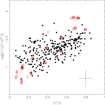
Figure 2: Ionic abundances $\rm S^{+}/(S^{+}+S^{2+})$ vs. $\rm O^{+}/O$. Black squares represent observational ionic determinations computed using the data from Table 5 and the Visible-lines method (see Sect. 4.2). Open circles represent ionic abundances predicted by our models (see Sect. 3). The error bar represents typical uncertainties as defined in Sect 4.1.

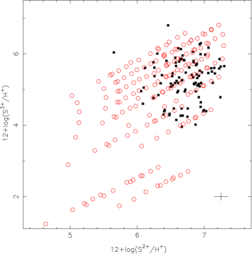
Figure 3: Such as Fig. 2 but for the Ionic abundances $\rm S^{3+}/H^{+}$ vs. $\rm S^{2+}/H^{+}$ computed using the IR-sample (Table 6) and the IR-lines method (see Sect. 4.2).

5 Results

5.1 Theoretical-ICF

We derived a theoretical ICF for the sulphur based on the photoionization model results described in Sect. 3. To verify how representative are our models of real H ii regions, in Fig. 2, the ionic abundance ratio $\rm S^{+}/(S^{+}+S^{2+})$ against the ionization degree $\rm O^{+}/O$ calculated from the data from Table 5 and using the Visible-lines method are compared with those predicted by the models. The theoretical ionic values considered are the ones weighted over the volume of the hypothetical nebulae. We can see that the models occupy the most part of the region where the observational data are located and they reproduce the tendency of $\rm S^{+}/(S^{+}+S^{2+})$ increases with $\rm O^{+}/O$. However, there is a region occupied by observational data with $[\rm S^{+}/(S^{+}+S^{2+})]\>\ga\>-1$ and $\rm(O^{+}/O)\>\ga\>0.2$ not covered by the models. This seems to be not crucial for the present analysis since similar ICFs can be derived from both models and observations, as we are presenting in this paper.

In Fig. 3, the $\rm S^{3+}/H^{+}$ and  $\rm S^{2+}/H^{+}$ abundances calculated using the IR-lines method and the IR-sample and those predicted by the models are shown. Again, we can see that the models cover the region occupied by the observations.

Figure 4: Ionization Correction Factor for the sulphur vs.  $\rm O^{+}/O$. Squares and triangles represent direct estimations (see Table 7) of the ICF taking into account the $\rm S^{2+}$ ionic abundance values estimated from the Visible-sample (Direc-Vis) and the IR-sample (Direct-IR), respectively. Circles represent estimations of our models. Curves represent the fittings to the Eq. 2: Solid line shows the best fit obtained using our models and dashed and dotted lines the ones obtained using the observational estimations, as indicated. The $\alpha$ values of the best fits are indicated in the legend. The error bars represent typical uncertainties as defined in Sect 4.2.

The predictions of the models were used to compute an ICF for the sulphur defined by:

$${\rm ICF(S^{+}+S^{2+})}=\frac{{\rm S/H}}{{\rm(S^{+}+S^{2+})/H^{+}}},$$ (16)

where $\rm S/H$ is the ratio between the total sulphur and the hydrogen abundances. Assuming the expression suggested by Stasińska (1978a) and presented in Eq. 2, we found $\alpha=3.27\pm 0.01$ from a fitting to our model results.

5.2 Direct ICFs

When emission-lines of the main ionization stages of an element are observed, it is possible to calculate the total abundance of the element and thus, derive an ICF. Therefore, following the methodology presented by Vermeij & van der Hulst (2002) and Pérez-Montero et al. (2006), we used the Visible and IR samples and the equations presented in Section 4 to derive direct values for the sulphur ICF for the common objects in both samples assuming

$${\rm ICF(S^{+}+S^{2+})}=\frac{{\rm S^{+}+S^{2+}+S^{3+}}}{{\rm S^{+}+S^{2+}}}.$$ (17)

This was possible only for nine objects. The $\rm S^{2+}$ can be estimated using the Visible data and/or using the IR data. Hence, for each object, we have two independent estimations of its sulphur ICF, these two values are named Direct-Vis and Direct-IR ICFs.

The identification of the nine objects for which was possible to compute the ICF by the procedure described above, the electron temperature ($t_{S3}$) and the ionic abundance values are listed in Table 7, while the $\rm O^{+}/O$ ratio and the ICF values are presented in Table 3. For Hubble V and I Zw 36 were only possible to compute the $\rm S^{2+}$ ionic abundance via the IR-method because the [S iii]$\lambda$9069,$\lambda$9532 emission-lines are not available in the literature. These are the only two objects in the subsample that do not fulfil the selection criterion to be in the Visible-sample but were included here because they contribute to a better estimation of the Direct-IR sulphur ICF. The difference in the $\rm S^{2+}$ abundances calculated from Visible and IR lines methods has an average value of $\sim$0.15 dex, with the maximum value of $\sim$0.35 dex. In the subsequent paper of this series, we will use photoionization models with abundance variations along the radius of the hypothetical nebula in order to investigate the source of this discrepancy.

In Fig. 4 the direct sulphur ICF values as a function of $\rm O^{+}/O$ are plotted together with the corresponding fittings. We found $\alpha=2.76\pm 0.22$ when $\rm S^{2+}$ is computed by the IR-method and $\alpha=3.08\pm 0.21$ when the Visible-method is considered. We can note in Fig. 4 that the two fits for the estimations based on IR and Visible methods (red and blue lines) seem to be not satisfactory for $\rm O^{+}/O\la 0.2$, i.e. for the regime of high excitation. Similar result was found by Vermeij & van der Hulst (2002). A larger number of direct ICF estimations for objects with high excitation is clearly need to improve the results for this regime.

The error in the Direct-ICF value is due to the uncertainties of ionic abundance determinations ($\rm S^{+},S^{2+},O^{+}$, and $\rm O^{2+}$) and due to the discrepancy between the abundance of $\rm S^{2+}$ calculated via Visible and IR methods (Dors et al., 2013; Vermeij & van der Hulst, 2002). Based on the results of Vermeij & van der Hulst (2002), we assumed an average error of 0.2 for the Direct-ICF and 0.15 for $\rm O^{+}/O$, obtained from ionic estimations of Kennicutt et al. (2003). These uncertainties yield an error in the total sulphur abundance of only $\sim$10%.

Table 2: Electron temperatures ($t_{S3}$) and sulphur ionic abundances estimated for the Visible and IR samples.

Object	$t_{\rm e}(10^{4}$K)	$\log(\rm S^{+}/H^{+})_{Vis}$	$\log(\rm S^{2+}/H^{+})_{Vis}$	$\log(\rm S^{2+}/H^{+})_{IR}$	$\log(\rm S^{3+}/H^{+})_{IR}$
N160A1	0.92	-6.24	-5.20	-5.31	-6.03
N160A2	0.88	-6.24	-5.18	-5.39	-6.22
N4A	0.94	-6.41	-5.27	-5.15	-5.93
N66	1.18	-6.53	-5.69	-5.72	-6.35
N157-B	1.29	-6.09	-5.49	-5.30	-6.57
N88-A	1.41	-6.87	-6.05	-6.40	-6.28
N81	1.26	-6.72	-5.81	-6.00	-6.62
Hubble Va	1.09	-6.68	—	-5.58	-6.21
I Zw 36a	1.61	-6.90	—	-5.81	-6.08

^aSee text for an explanation about the inclusion of these two particular objects.

Table 3: $\rm O^{+}/O$ ionic abundances and direct sulphur ICFs estimations using the Visible-lines and the IR-lines methods.

Object	$\rm O^{+}/O$	ICF
		Vis	IR
N160A1	0.256	1.13	1.17
N160A2	0.272	1.08	1.13
N4A	0.238	1.20	1.16
N66	0.192	1.20	1.20
N157-B	0.404	1.07	1.04
N88-A	0.126	1.60	1.98
N81	0.202	1.15	1.20
Hubble V	0.194	—	1.21
I Zw 36	0.120	—	1.49

6 Discussion

In their pioneer paper, Peimbert & Costero (1969) obtained photoelectric observations of the H ii regions Orion, M 8 and M 17 and suggested that the total abundance of the sulphur can be obtained by using an ICF defined by the ionic abundance ratio ($\rm O^{+}+O^{2+}$)/$\rm O^{+}$. This empirical approach is based on the similarity between the ionization potentials of $\rm S^{2+}$ and $\rm O^{+}$. During the next decades, sulphur ICFs had been mainly derived from the analytical expression suggested by Stasińska (1978a), and the $\alpha$ value of this original prescription have been largely discussed. For example, data obtained with the Infrared Space Observatory by Vermeij et al. (2002) became, possibly, the first test for the $\alpha$ value, since direct estimations of sulphur ICFs were possible. These authors showed that an $\alpha$ value equal to 2, as suggested by French (1981), overpredicts the $\rm S^{3+}$ ionic abundance, in concordance with the result previously obtained by Garnett (1989). From their observational data, Vermeij & van der Hulst (2002) concluded that $\alpha=3$ is a more reliable value, at least for $\rm O^{+}/O>0.2$.

Despite ICFs could be obtained from direct calculation of ionic abundances (Vermeij & van der Hulst, 2002) or even from ionization potential considerations (e.g. Peimbert & Costero 1969; French 1981), ICFs based on grids of photoionization models of nebulae are more reliable because all ionization stages of a given ion as well as several physical processes (e.g. charge transfer reactions) are taken into account in the calculations (Stasińska, 2002). In the present work, we built a grid of photoionization models assuming a large range of nebular parameters (e.g. $Z$, $U$, S/O) and derived a theoretical sulphur ICF. Based on the agreement between the model predictions and data of a large sample of objects, we suggested an $\alpha$ value of $3.27\pm 0.01$ in the Stasińska formulae. This value is somewhat higher than the one derived by Vermeij & van der Hulst (2002), but it is in consonance with the one derived through direct ionic estimations ($\alpha=3.08\pm 0.21$) based mainly on the Visible-line method (Direct-Vis ICF).

With the aim to compare the S/H total abundances yielded by the use of different ICFs, we considered the relation:

$$\rm\frac{S}{H}=ICF(S)\>\times\>\frac{S^{+}+S^{2+}}{H^{+}},$$ (18)

using the $\rm S^{+}$ and $\rm S^{2+}$ ionic abundances estimated for the objects in our Visible-sample via the Visible-lines method. Firstly, we compared the S/H abundances derived through the Theoretical ICF ($\alpha=3.27\pm 0.01$), with those derived using the Direct-Vis ICF ($\alpha=3.08\pm 0.21$) and the Direct-IR ICF ($\alpha=2.76\pm 0.22$). In panels a of Fig. 5 these comparisons are shown. In this figure we also plotted the differences (D) between the S/H total abundances estimations (panels b) and the $\rm O^{+}/O$ ratio (panels c). It can be seen that the Theoretical ICF yields S/H total abundances in excellent agreement with those given by the Direct-Vis and Direct-IR ICFs, with an average difference $\rm<D>\approx 0.00$ and dispersions of 0.005 dex and 0.01 dex respectively, independently of the ionization degree that is sampled by the $\rm O^{+}/O$ ratio.

Figure 5: Panel a: comparison between the S/H total abundances obtained for the objects in the Visible-sample applying the Theoretical ICF and, Direct-Vis (left plot) and Direct-IR (right plot) ICFs, as indicated. Panel b: differences between the estimations using the considered ICFs with they average value ($\rm<D>$) and its dispersion ($\sigma$) indicated. Panel c: $\rm O^{+}/O$ ratio for each estimation.

Figure 6: Idem Fig. 5 for different ICFs from the literature, as indicated.

Figure 7: Idem Fig. 5 for the ICF proposed by Delgado-Inglada et al. (2014)

Secondly, we also compare the S/H total abundance estimations based on our Theoretical ICF with the ones obtained using some ICFs proposed in the literature. In what follows a brief description of these ICFs is presented.

• Kennicutt et al. ICF– Kennicutt et al. (2003) proposed to use $\alpha=2.5$ for typical H ii regions. This is an average value obtained from the photoionization models grid calculated by Garnett (1989). The same $\alpha$ value was obtained by Pérez-Montero et al. (2006) from optical and IR data.

• Izotov et al. ICF– Izotov et al. (2006a) used a grid of photoionization models by Stasińska & Izotov (2003) built assuming spectral energy distributions calculated with the $Starburst99$ (Leitherer et al., 1999) and stellar atmosphere models by Smith et al. (2002) to derive an expression for the sulphur ICF. These authors derived ICFs considering three metallicity regimes: low [$\rm 12+\log(O/H)\><\>7.6$], intermediate [$\rm 7.6\><\>12+log(O/H)\><\>8.2$] and high [$\rm 12+log(O/H)\>>\>8.2$], which are given by:

  $${\rm ICF}({\rm S})\!\!\!\! = \!\!\!\!0.121x+0.511+0.161/x,\ {\rm low\ }Z,$$

  $$= \!\!\!\!0.155x+0.849+0.062/x,\ {\rm inter.\ }Z,$$

  $$= \!\!\!\!0.178x+0.610+0.153/x\,\,\,\ {\rm high\ }Z,$$

  where $x=\rm O^{+}/O$.

• Thuan et al. ICF– Thuan et al. (1995), who used the results of photoionization models grid built by Stasińska (1990) and NLTE atmosphere models by Mihalas (1972), derived

  $${\rm ICF}\!=\!\Big{[}0.013+x\,\big{[}5.10+x\,\big{(}-12.78+x\,(14.77-6.11\,x)\big{)}\big{]}\Big{]}^{-1}.$$

• Kwitter & Henry ICF– Kwitter & Henry (2001) built a grid of photoionization models considering a blackbody as the ionizing source in order to derive sulphur ICFs for planetary nebulae that, in principle, it can be employed for H ii regions. These authors proposed

  $${\rm ICF(S)}=e^{-0.017+(0.18\,\beta)-(0.11\,\beta^{2})+(0.072\,\beta^{3})},$$

  where $\beta=\rm\log(O/O^{+})$.

• Delgado-Inglada et al. ICF — Delgado-Inglada et al. (2014) computed a large grid of photoionization models in order to derive new formulae for ICFs of several elements to be applied in studies of planetary nebulae. The expression derived by these authors to calculate the total abundance S/H can be to write in the form

  $$\rm\frac{S}{H}=ICF(S)\>\times\>\frac{S^{+}+S^{2+}}{O^{+}}\>\times\>\frac{O}{H},$$

  where

  $${\rm ICF(S)}=\frac{-0.02-0.03w-2.31w^{2}+2.19w^{3}}{0.69+2.09w-2.69w^{2}},$$

  and

  $$w=\rm O^{2+}/O.$$

In Fig. 6 (panels a) a comparison between S/H total abundance estimations based on our Theoretical ICF and those from the literature are shown. In this figure we also show the difference (D) between these estimations (panels b) and the $\rm O^{+}/O$ ratio (panels c). Taking into account the typical errors found in the S/H total abundance estimations (see e.g. Hägele et al., 2008) and the dispersion ($\sigma$) of the average differences ($\rm<\!D\!>$), it might seem that the different S/H estimations are in agreement. However, with exception of the ICF of Izotov et al. (2006a), there are clear systematic differences between the values derived through the use of our Theoretical ICF and from the other ICFs. Moreover, difference in S/H abundances obtained from distinct ICFs can be not negligible when only an individual object is considered. In fact, we noted that it could reach up to about 0.3 dex for the low metallicity regime (see Fig. 5).

Concerning the ratio between sulphur and oxygen abundances, several studies have addressed the investigation about the variation of S/O with O/H in individual galaxies (e.g. Croxall et al. 2015; Berg et al. 2013; Skillman et al. 2013; López-Sánchez & Esteban 2009; Kennicutt et al. 2003; Vermeij & van der Hulst 2002; Garnett et al. 1997; Christensen et al. 1997; Vílchez et al. 1988) or in a general context (e.g. Guseva et al. 2011; Hägele et al. 2008, 2012; Pérez-Montero et al. 2006; Kehrig et al. 2006; Henry & Worthey 1999; Izotov et al. 1997). Most of these results indicates that the ratio S/O appears to be constant with the metallicity, which argues that either these elements are produced by massive stars within a similar mass range or by stars with a distinct mass interval but being formed with an universal IMF (Henry & Worthey, 1999). However, when a large sample of data is considered, the dispersion found is very large and the assumption of a constant S/O ratio is questionable (Hägele et al., 2008, 2012; Pérez-Montero et al., 2006; Kehrig et al., 2006). Therefore, with the goal of studying the relation of the S/O ratio with the metallicity (traced by the O/H abundance), we used the data listed in Table 5 and all the ICFs considered in the present work to calculate S/O and O/H ratios via the Visible-lines method. The Direct-Vis ICF was not considered since its $\alpha$ value is very similar to that of the Theoretical one. In Fig. 8 only the estimations obtained from the Theoretical ICF is shown. For estimations from other ICFs (not shown), similar results were obtained. The solar values $\rm\log(S/O)_{\odot}=-1.43$ and $\rm 12+\log(O/H)_{\odot}=8.69$ derived using the sulphur abundance from Grevesse & Sauval (1998) and the oxygen one from Allende Prieto et al. (2001) are also indicated. We can see in this figure that most of the objects present subsolar S/O and O/H abundance ratios. Interestingly, for the extreme low metallicity regime, some of the objects reach very high S/O abundance ratios. Since the dispersion is high and the number of objects is much lower than for the high metallicty regime, more data are needed to confirm this result.

We also performed a fit to these data, assuming a linear regression without taking into account the individual errors. In Table 8, the coefficients of the fittings, and the linear regressions considering all ICFs are listed. We found that the S/O ratio decreases with metallicity, yielding a mean slope of about $-0.27$ with all the fitted slopes in agreement within the estimated errors. We also obtained the average values for log(S/O) estimated via the different ICFs and considering the three different metallicity regimes. These values and the number of objects used to calculate them are also listed in Table 8. Considering all the metallicity regimes together and all the considered ICFs we found an average $<\log(\rm S/O)>=-1.72\pm 0.03$. Despite the dispersion, when low, intermediate and high metallicities regimes are separately considered, we note a decrease in S/O when the metallicity increases. For low and high metallicity regimes we derived mean values of $<\log(\rm S/O)>$ $-1.53\pm 0.05$ and $-1.78\pm 0.02$, respectively. Similar results were also derived by Díaz et al. (1991), Vílchez et al. (1988) for M51 and M33 galaxies and by Shaver et al. (1983) for Milk Way.

Table 4: Coefficients of the linear regressions $\rm\log(S/O)=\>a\times\>\big{[}12+\log(O/H)\big{]}+b$ fitted to the data plotted in Fig. 8 taking into account each of the considered ICF. Mean values for the abundance ratio $\rm\log(S/O)$ considering all the metallicity range as well as the corresponding ones for the low [$\rm 12+\log(O/H)\><\>7.6$], intermediate [$\rm 7.6\><\>12+log(O/H)\><\>8.2$] and high [$\rm 12+log(O/H)\>>\>8.2$] metallicity regimes, and the number of objects used in these calculations are shown.

			$<\log(\rm S/O)>$
			Metallicity regime
	a	b	All	Low	Interm.	High
Number objects			261	14	114	133
ICF
Direct-IF	$-0.28\pm 0.04$	0.60$\pm 0.33$	$-1.71\pm 0.22$	$-1.52\pm 0.36$	$-1.66\pm 0.20$	$-1.78\pm 0.20$
Theoretical	$-0.26\pm 0.04$	0.45$\pm 0.33$	$-1.73\pm 0.22$	$-1.55\pm 0.38$	$-1.68\pm 0.20$	$-1.79\pm 0.19$
Kennicut et al.	$-0.30\pm 0.04$	0.72$\pm 0.33$	$-1.70\pm 0.22$	$-1.50\pm 0.35$	$-1.64\pm 0.20$	$-1.77\pm 0.20$
Izotov et al.	$-0.28\pm 0.04$	0.60$\pm 0.33$	$-1.73\pm 0.22$	$-1.53\pm 0.31$	$-1.68\pm 0.20$	$-1.80\pm 0.20$
Thuan et al.	$-0.32\pm 0.04$	0.94$\pm 0.33$	$-1.66\pm 0.23$	$-1.44\pm 0.32$	$-1.59\pm 0.20$	$-1.73\pm 0.20$
Kwitter & Henry	$-0.23\pm 0.04$	0.13$\pm 0.34$	$-1.75\pm 0.22$	$-1.59\pm 0.41$	$-1.71\pm 0.21$	$-1.79\pm 0.19$
Delgado-Inglada et al.	$-0.26\pm 0.04$	0.41$\pm 0.33$	$-1.75\pm 0.22$	$-1.56\pm 0.38$	$-1.71\pm 0.21$	$-1.81\pm 0.19$

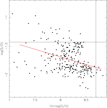
Figure 8: Relation between log(S/O) and 12+log(O/H) ratios using the Visible-lines method and our Theoretical ICF. Black lines represent the solar S/O and O/H abundance ratios derived using the oxygen abundance from Allende Prieto et al. (2001) and sulphur abundance from Grevesse & Sauval (1998). Red lines represent linear regressions to the observational estimations. Coefficients of this regression are given in Table 8.

7 Conclusions

We built a grid of photoionization models combined with stellar population synthesis models to derive Ionization Correction Factors (ICFs) for the sulphur. The reliability of these ICFs was obtained from the agreement between ionic abundances predict by the models and those calculated through optical and infrared spectroscopic data of star-forming regions with a very wide range in metallicity ($\rm 7.0\>\la\>12+\log(O/H)\>\la 8.8$) and ionization degree ($\rm 0.1\>\la\>O^{+}/O\>\la 0.9$). From our results, we suggest $\alpha=3.27\pm 0.01$ to be used in the classical Stasińska formula. This $\alpha$ value is in consonance with the one derived from direct estimations based on spectroscopic data of a small sample of objects. A comparison of the S/H total abundance derived by us for the objects in our visible sample and considering different ICFs proposed in the literature was performed. Although, in average, the differences between these determinations are similar to the uncertainties in the S/H estimations, we noted that it could reach up to about 0.3 dex for the low metallicity regime. Finally, the highest S/O abundance ratios are derived for objects with extreme low metallicity values. Indeed, a tendency of the S/O ratio to decrease with the metallicity was found, independently of the considered ICF.

8 Appendix

Table 5: Dereddened line fluxes (relative to H$\beta$=100.0) compiled from the literature. The intensity of the line [O ii]$\lambda$3727 represents the sum of the lines [O ii]$\lambda$$\lambda$3726+ 29

Object	[O ii]$\lambda$3727	[O iii]$\lambda$4363	[O iii]$\lambda$5007	[S ii]$\lambda$6717	[S ii]$\lambda$6731	[S ii]$\lambda$6725b	[S iii]$\lambda$9069	Ref.
H1105	185.0	1.4	316.0	13.1	11.0	—	36.2a	1
H1159	198.0	1.9	317.0	17.6	12.2	—	27.7a	1
H1170	308.0	1.6	201.0	33.4	23.3	—	48.6a	1
H1176	160.0	2.4	369.0	13.4	9.6	—	32.4a	1
H1216	151.0	4.7	473.0	11.0	7.9	—	23.7a	1
H128	145.0	1.7	391.0	13.3	10.0	—	29.8a	1
H143	219.0	2.3	284.0	23.2	17.0	—	26.8a	1
H149	212.0	1.8	318.0	21.1	16.1	—	27.2a	1
H409	218.0	2.3	370.0	17.2	14.0	—	25.7a	1
H67	244.0	3.5	342.0	15.6	10.7	—	26.3a	1
N5471-A	106.0	9.5	644.0	8.7	7.1	—	17.5a	1
N5471-B	213.0	6.6	395.0	29.1	25.6	—	14.5a	1
N5471-C	174.0	5.4	416.0	13.1	10.1	—	18.8a	1
N5471-D	137.0	8.0	578.0	11.7	8.9	—	21.6a	1
N160A1	165.5	2.4	423.6	12.7	10.1	—	37.9	2
N160A2	164.6	1.8	382.1	11.7	9.3	—	35.3	2
N157B	223.0	4.8	324.0	29.1	24.5	—	35.6	2
N79A	233.0	2.4	306.0	15.1	12.5	—	38.3	2
N4A	152.2	2.6	430.0	9.1	6.9	—	34.7	2
N88A	95.6	12.0	672.0	5.2	4.5	—	17.5	2
N66	116.9	5.6	469.0	10.1	7.0	—	20.7	2
N81	137.0	7.4	528.0	6.9	5.2	—	18.0	2
SDSS J1455	111.54	10.22	613.55	10.00	7.88	—	11.54	3
SDSS J1509	153.18	4.20	499.42	19.66	14.88	—	25.46	3
SDSS J1528	228.82	5.00	489.32	19.23	14.22	—	16.88	3
SDSS J1540	217.93	2.91	309.42	26.09	19.19	—	20.95	3
SDSS J1616	84.91	8.51	615.16	7.74	5.81	—	16.47	3
SDSS J1729	176.22	6.60	515.41	12.86	10.09	—	20.92	3
1	243	3.38	321	—	—	22.1	17.0	4
2	166	5.59	504	—	—	17.4	19.6	4
3	373	1.16	119	—	—	52.0	12.7	4
4	286	2.14	253	—	—	33.2	20.7	4
5	296	1.10	226	—	—	52.7	26.4	4
6	275	1.16	246	—	—	38.6	20.3	4
8	307	0.77	144	—	—	44.2	20.6	4
9	172	0.89	235	—	—	33.1	27.2	4
10	180	0.91	236	—	—	16.3	26.5	4
11	258	1.11	201	—	—	41.8	23.8	4
14	248	0.75	181	—	—	41.6	29.6	4
17	213	0.59	192	—	—	27.3	27.3	4
19	192	0.61	165	—	—	30.6	23.1	4
20	146	0.71	227	—	—	20.0	28.6	4
23	176	0.57	198	—	—	28.0	24.0	4
24	197	0.62	180	—	—	30.3	26.5	4
26	160	1.19	259	—	—	22.1	28.2	4
27	357	1.59	178	—	—	81.7	17.3	4
28	314	1.89	244	—	—	37.2	21.2	4
VCC1699	126.0	4.1	553.1	10.4	7.7	—	15.7	5
SDSS J002101.03	163.4	5.6	433.4	13.6	10.7	—	11.9	6
SDSS J003218.60	157.3	6.2	460.7	17.3	12.5	—	21.7	6
SDSS J162410.11	147.1	7.0	564.2	13.6	9.9	—	16.0a	6
SDSS J165712.75 (A)	188.32	5.24	430.82	22.07	15.98	—	14.00	7
SDSS J165712.75 (B)	132.66	8.46	486.53	14.89	10.60	—	9.84	7
SDSS J165712.75 (C)	148.09	8.38	447.27	16.99	11.54	—	17.77	7
SBS 0335-2013052E	20.11	11.08	327.89	1.94	1.51	—	12.53	8
UM 283D	204.65	4.10	336.63	29.30	20.80	—	20.72	9
UM 133H	107.18	7.72	367.90	9.40	6.94	—	7.42	9
HE 2-10C	211.87	1.96	150.52	14.69	17.87	—	34.18	9
HE 2-10E	193.03	0.26	126.64	14.10	15.94	—	27.71	9

Table 5: -$continued$

Object	[O ii]$\lambda$3727	[O iii]$\lambda$4363	[O iii]$\lambda$5007	[S ii]$\lambda$6717	[S ii]$\lambda$6731	[S ii]$\lambda$6725b	[S iii]$\lambda$9069	Ref.
NGC 3125	93.12	5.13	578.95	11.97	9.92	—	31.97	9
Mrk 1259	170.87	1.08	161.78	15.75	18.13	—	23.74	9
POX 4	81.26	9.12	652.36	7.63	5.94	—	12.31	9
TOL 1214-277	30.82	17.29	511.82	2.24	1.39	—	2.85	9
J 1253-0312	84.22	10.37	665.63	4.94	6.25	—	13.74	9
NGC 5253 No.C1	96.34	7.45	634.27	7.79	7.79	—	22.44	9
NGC 5253 No.C2	148.48	3.09	445.98	14.80	12.20	—	21.57	9
NGC 5253 No.P2	106.83	7.92	649.56	7.19	8.00	—	22.82	9
TOL 89 No.1	151.60	3.38	489.58	11.67	8.99	—	24.83	9
TOL 89 No.2	157.62	1.94	385.19	24.69	18.48	—	50.12	9
TOL 1457-262	258.97	6.80	627.73	11.99	9.03	—	13.90	9
TOL 1924-426 No.1	94.48	5.36	436.15	9.56	7.31	—	13.07	9
TOL 1924-426 No.2	113.90	6.23	531.57	10.88	8.59	—	13.98	9
NGC 6822 V	78.55	5.18	530.38	6.03	4.62	—	25.60	9
VS 3	226.0	1.0	147.0	19.0	13.5	—	25.1	10
VS 49	219.0	2.9	239.0	23.8	16.9	—	25.5	10
VS 48	252.0	3.8	314.0	20.9	15.9	—	26.8	10
NGC 604	215.2	0.75	207.7	16.6	11.1	—	3.98	11
NGC 588	148.2	2.4	464.7	11.8	7.7	—	5.63	11
Leo P	46.5	3.8	145.3	3.6	2.7	—	14.5	12
IC 132-A	150.7	6.7	500.1	8.9	5.7	—	27.5	13
IC 132-B	164.7	6.4	485.6	9.9	6.6	—	24.0	13
IC 132-C	192.4	7.7	463.5	11.7	7.6	—	28.4	13
IC 132-D	210.5	8.4	449.1	12.7	8.4	—	30.8	13
IC 132-E	204.5	10.7	443.5	12.3	8.2	—	30.6	13
IC 132-F	188.9	11.2	445.1	11.5	7.3	—	28.1	13
IC 132-G	221.6	14.0	435.0	12.9	8.6	—	28.2	13
IC 132-H	241.3	18.9	433.3	14.0	9.2	—	23.4	13
IC 132-I	267.2	29.0	444.6	16.1	9.5	—	18.9	13
8	150	0.34	27	44	36	—	19	14
17	143	0.40	114	15	11	—	23	14
25	158	1.30	251	10.9	7.9	—	21	14
26	230	1.20	220	17.7	12.4	—	22	14
35	150	1.35	320	12.7	9.2	—	21	14
32	269	0.97	102	39	29	—	16	14
II Zw 40	83.9	10.9	740.9	6.7	5.4	—	13.9	15
Mrk 5	212.9	4.4	381.5	23.3	16.6	—	15.9	15
0749+568	166.8	9.8	488.0	17.8	11.4	—	12.7	15
0926+606	178.5	8.3	477.2	18.2	14.6	—	12.2	15
Mrk 709	183.6	8.8	369.6	31.3	28.5	—	8.7	15
Mrk 22	148.7	8.2	545.5	11.4	8.5	—	14.8	15
Mrk 1434	96.8	10.4	502.8	9.6	6.7	—	9.2	15
Mrk 36	129.3	9.6	483.4	11.7	8.4	—	11.9	15
VII Zw 403	133.3	7.1	345.5	10.3	7.5	—	11.7	15
UM 461	52.7	13.6	602.2	5.2	4.2	—	12.4	15
UM 462	174.2	7.8	492.9	16.8	11.2	—	10.5	15
Mrk 209	71.9	12.7	554.3	6.1	4.5	—	12.2	15
A	245	1.7	134.1	41.9	32.5	—	20.8	16
N110	182	1.3	140	29	28	—	27.0	16
B	242	3.1	357	30.6	22.4	—	14.2	16
C	280	1.7	257	33	24	—	13.0	16
N	173	1.2	152	30	29	—	31.0	16
SE	46.6	4.4	189	—	—	7.2	3.9	17
NW	26.4	6.2	185	—	—	3.8	3.0	17

Table 5: -$continued$

Object	[O ii]$\lambda$3727	[O iii]$\lambda$4363	[O iii]$\lambda$5007	[S ii]$\lambda$6717	[S ii]$\lambda$6731	[S ii]$\lambda$6725b	[S iii]$\lambda$9069	Ref.
N12A	191	3.7	368.4	9.2	7.4	—	19.9	18
N13AB	216.3	2.7	347.6	13.4	8.4	—	23.6	18
N4A	203.5	2.6	394.4	13.4	11.0	—	36.7	18
N138A	179.1	2.1	371.0	8.0	6.2	—	28.0	18
Haro 15-B	90.5	7.8	698	7.3	5.9	—	11.9	19

References— Data compiled by (1) Kennicutt et al. (2003), (2) Vermeij et al. (2002), (3) Hägele et al. (2008), (4) Bresolin et al. (2009),

(5) Vílchez & Iglesias-Páramo (2003) (6) Hägele et al. (2006), (7) Hägele et al. (2011), (8) Izotov et al. (2006b), (9) Guseva et al. (2011),

(10) Garnett et al. (1997), (11) Vílchez et al. (1988), (12) Skillman et al. (2013), (13) López-Hernández et al. (2013),

(14) Zurita & Bresolin (2012), (15) Pérez-Montero & Díaz (2003), (16) González-Delgado et al. (1995),

(17) Skillman & Kennicutt (1993), (18) Russell & Dopita (1990), (19) Hägele et al. (2012). ^aValue computed from

$I$([S iii]$\lambda$9069= 0.4 $\times$ $I$([S iii]$\lambda$9532). ^bSum of the emission-line intensities [S ii]$\lambda$6717 and $\lambda$6731.

Table 6: Fluxes of infrared emission-lines (in $\rm W/cm^{2}$) compiled from the literature.

Object	H I 4.05 $\mu$m	[S iv] 10.51$\mu$m	[S iii]18.71$\mu$m	Flux $\rm W/cm^{2}$	Reference
IR 02219	6.6	26	59	$10^{-18}$	19
IR 02219	6.7	28	43	$10^{-18}$	19
IR 10589	1.71	1.5	15.7	$10^{-18}$	19
IR 11143	0.68	8.4	7.8	$10^{-18}$	19
IR 12063	2.08	9.1	11.8	$10^{-18}$	19
IR 12073	6.6	59	35	$10^{-18}$	19
IR 12331	0.51	1.28	9.3	$10^{-18}$	19
IR 15384	2.86	2.6	25.9	$10^{-18}$	19
IR 15502	1.5	0.23	4.9	$10^{-18}$	19
IR 16128	0.63	0.82	6.4	$10^{-18}$	19
IR 17221	0.64	0.13	7.3	$10^{-18}$	19
IR 17455	2.0	1.9	23.2	$10^{-18}$	19
IR 18317	2.00	0.33	25.6	$10^{-18}$	19
IR 18434	6.80	4.2	46	$10^{-18}$	19
IR 18502	0.89	0.49	8.6	$10^{-18}$	19
IR 19207	0.67	1.41	7.4	$10^{-18}$	19
IR 19598	4.7	3.3	7.6	$10^{-18}$	19
IR 21190	2.25	2.09	6.51	$10^{-18}$	19
IR 23030	1.60	1.3	16.3	$10^{-18}$	19
IR 23133	1.74	0.20	10.0	$10^{-18}$	19
N160A1	51.7	289	317	$10^{-20}$	20
N160A2	55.2	194	268	$10^{-20}$	20
N159-5	12.6	56.7	74.2	$10^{-20}$	20
N4A	10.7	75.9	93.6	$10^{-20}$	20
N83B	12.3	18.1	28.8	$10^{-20}$	20
N157B	6.3a	11.7	46.5	$10^{-20}$	20
N88A	14.5a	55.1	8.89	$10^{-20}$	20
N81	9.7a	15.9	14.1	$10^{-20}$	20
NGC3603c	101.07b	186.94	691.99	$10^{-20}$	21
30 Dorc	168.02b	811.68	802.4	$10^{-20}$	21
N66c	8.754b	25.72	23.44	$10^{-20}$	21
638	1.37b	4.94	3.09	$10^{-20}$	22
623	2.98b	7.45	5.04	$10^{-20}$	22
45	3.55b	10.1	17.4	$10^{-20}$	22
214	1.39b	54.2	5.18	$10^{-20}$	22
33	0.901b	1.22	4.91	$10^{-20}$	22
42	0.625b	0.573	2.56	$10^{-20}$	22
32	0.657b	0.238	1.48	$10^{-20}$	22
251	1.00b	1.57	3.02	$10^{-20}$	22
301	0.915b	0.475	4.69	$10^{-20}$	22
4	1.78b	1.46	7.80	$10^{-20}$	22
79	3.00b	7.70	23.1	$10^{-20}$	22
87E	9.30b	5.29	49.1	$10^{-21}$	22
302	9.65b	7.26	39.8	$10^{-21}$	22
95	6.10b	6.95	36.8	$10^{-21}$	22
710	1.51b	0.659	4.05	$10^{-20}$	22
691	1.18b	4.43	6.43	$10^{-20}$	22
Orion	1.448b	4.765	14.49	$10^{-10}$	23
G333-North	2.932b	0.256	14.52	$10^{-11}$	24
G333-West	2.93b	0.164	17.51	$10^{-11}$	24
NGC 1222	15.05b	22.24	64.80	$10^{-21}$	18
IC 342	44.16b	4.76	320.03	$10^{-21}$	18
NGC 1614	12.56b	6.89	83.03	$10^{-21}$	18
NGC 2146	48.35b	6.30	190.12	$10^{-21}$	18
NGC 3256	43.94b	5.25	171.83	$10^{-21}$	18
NGC 3310	4.11b	4.46	20.50	$10^{-21}$	25
NGC 4676	3.40b	0.56	11.32	$10^{-21}$	25
NGC 4818	12.14b	2.21	71.96	$10^{-21}$	25
NGC 7714	15.47b	14.76	81.50	$10^{-21}$	25

Table 6: -$continued$

Object	HI 4.05 $\mu$m	[SIV] 10.51$\mu$m	[SIII]18.71$\mu$m	Flux $\rm W/cm^{2}$	Reference
W3 IRS 5	3.5	3.3	16.6	$10^{-19}$	26
W3 IRS 2	63.3	228	570	$10^{-19}$	26
W3 IRS 2	63.5	259	414	$10^{-19}$	26
ORIONc	373.9	1116.7	3659.0	$10^{-19}$	26
Caswell H2O 287.37- 00.62	1.6	2.8	29.8	$10^{-19}$	26
TRUMPLER14	6.4	9.6	68.7	$10^{-19}$	26
Gal 287.39-00.63	5.6	34.0	63.7	$10^{-19}$	26
Gal 289.88-00.79	16.3	14.6	149.0	$10^{-19}$	26
NGC 3603	1.7	15.7	25.4	$10^{-19}$	26
RAFGL 4127	6.6	75.7	72.9	$10^{-19}$	26
Gal 298.23-00.33	65.9	557.0	382.0	$10^{-19}$	26
GRS 301.11 +00.97	4.7	11.5	77.3	$10^{-19}$	26
GRS 326.44+00.91	26.4	25.5	254.0	$10^{-19}$	26
15408-5356	29.7	53.4	441.0	$10^{-19}$	26
G327.3-0.5	28.7	27.5	497.0	$10^{-19}$	26
GRS 328.30+00.43	14.7	2.4	48.8	$10^{-19}$	26
15567-5236	25.7	6.4	40.4	$10^{-19}$	26
16172-5028	12.7	4.8	136.0	$10^{-19}$	26
G333.13-0.43	4.4	12.0	100.0	$10^{-19}$	26
Gal 337.9-00.5	15.2	30.0	255.0	$10^{-19}$	26
17059-4132	17.7	6.7	398.0	$10^{-19}$	26
NGC 6334-A	5.0	6.8	44.3	$10^{-19}$	26
NGC637I	11.5	51.0	251.0	$10^{-19}$	26
Gal 351.47-00.46	5.5	1.5	63.1	$10^{-19}$	26
NGC 6357IIIB	4.0	9.6	86.4	$10^{-19}$	26
RAFGL 2003	46.6	5.8	149.0	$10^{-19}$	26
ARCHFILc	13.91	0.9	133.2	$10^{-19}$	26
Pistol star	7.1	1.3	32.2	$10^{-19}$	26
SGR D H II	18.8	16.8	201.0	$10^{-19}$	26
RAFGL 2094	11.1	1.7	138.0	$10^{-19}$	26
M 17 c	184.23	1087.1	2457.2	$10^{-19}$	26
18317-0757	18.8	2.9	260.0	$10^{-19}$	26
RAFGL 2245	13.9	39.0	357.0	$10^{-19}$	26
Gal 033.91+00.11	8.8	59.9	5.1	$10^{-19}$	26
Gal 045.45+00.06	12.0	19.8	119.0	$10^{-19}$	26
Gal 049.20-00.35	6.4	12.1	76.6	$10^{-19}$	26
W51 IRS2	77.4	137.0	337.0	$10^{-19}$	26
IR 070.29+0160c	89.8	57.6	153.0	$10^{-19}$	26
S128 A	2.5	4.0	21.0	$10^{-19}$	26
S138	6.0	1.1	44.0	$10^{-19}$	26
S156 A	15.5	11.8	170.0	$10^{-19}$	26
S159	16.4	1.9	101.0	$10^{-19}$	26
Hubble V	1.9	7.5	6.7	$10^{-20}$	27
I Zw 36	1.9	12	4.9	$10^{-21}$	27

References— (19) Data compiled from Peeters et al. (2002), (20) Vermeij et al. (2002) , (21) Lebouteiller et al. (2008),

(22) Rubin et al. (2008), (23) Simpson et al. (1998), (24) Simpson et al. (2012), (25)Bernard-Salas et al. (2009),

(26) Giveon et al. (2002), and (27) Nollenberg et al. (2002). ^aFlux computed from H i 4.051$\mu$m/H i 2.63$\mu$m=1.74.

^bFlux computed from H i 4.051$\mu$m/H i 12.37$\mu$m=8.2. ^cFlux obtained assuming the measurements at the different observed positions.

Table 7: Electron temperature, electron density, ionic and total oxygen abundances for the sample of objetcs listed in Table 5. The estimations were calculated following the Visible-lines method described in Section 4.1. For the cases where was not possible to calcule the electron density, a value of $N_{\rm e}=200\>\rm cm^{-3}$ was assumed.

Object	$T_{\rm e}$ ($10^{4}$) K	$N_{\rm e}$ ($\rm cm^{-3}$)	$\log(\rm O^{+}/H^{+})$	12+log(O/H)	$\log(\rm S^{+}/H^{+})$	$\log(\rm S^{+2}/H^{+})$
H1105	0.9046	211	7.92	8.39	5.85	6.87
H1159	0.9721	—	7.84	8.29	5.89	6.68
H1170	1.0512	—	7.93	8.16	6.10	6.85
H1176	0.9931	37	7.72	8.27	5.76	6.73
H1216	1.1277	37	7.53	8.17	5.58	6.47
H128	0.9008	95	7.82	8.43	5.84	6.79
H143	1.0566	58	7.77	8.16	5.95	6.59
H149	0.9582	101	7.89	8.32	5.99	6.69
H409	0.9813	176	7.87	8.33	5.90	6.64
H67	1.1390	—	7.73	8.13	5.71	6.51
N5471-A	1.3090	188	7.21	8.07	5.40	6.22
N5471-B	1.3817	301	7.46	7.91	5.91	6.09
N5471-C	1.2428	115	7.48	8.02	5.60	6.29
N5471-D	1.2750	99	7.35	8.08	5.53	6.33
N160A1	0.9584	147	7.78	8.38	5.78	6.81
N160A2	0.9172	145	7.84	8.41	5.78	6.82
N157B	1.3113	232	7.53	7.93	5.93	6.51
N79A	1.0466	200	7.81	8.20	5.80	6.73
N4A	0.9743	94	7.72	8.35	5.61	6.74
N88A	1.4242	228	7.08	7.98	5.14	5.95
N66	1.2037	—	7.35	8.06	5.49	6.32
N81	1.2815	88	7.34	8.04	5.30	6.19
SDSS J1455	1.3798	142	7.18	7.99	5.42	6.04
SDSS J1509	1.0688	93	7.61	8.26	5.88	6.49
SDSS J1528	1.1384	67	7.70	8.22	5.82	6.30
SDSS J1540	1.1073	62	7.71	8.12	5.97	6.44
SDSS J1616	1.2747	83	7.14	8.07	5.35	6.20
SDSS J1729	1.2362	136	7.49	8.10	5.60	6.31
1	1.1503	—	7.72	8.10	5.63	6.31
2	1.1716	—	7.53	8.15	5.51	6.36
3	1.1205	—	7.93	8.06	6.02	6.21
4	1.0707	—	7.87	8.17	5.86	6.46
5	0.9241	—	8.09	8.36	6.18	6.71
6	0.9174	—	8.07	8.37	6.05	6.61
8	0.9449	—	8.07	8.26	6.08	6.58
9	0.8742	—	7.93	8.35	6.02	6.79
10	0.8776	—	7.95	8.35	5.71	6.77
11	0.9524	—	7.99	8.26	6.05	6.64
14	0.8913	—	8.06	8.33	6.10	6.80
17	0.8371	—	8.09	8.41	5.98	6.84
19	0.8698	—	7.99	8.29	5.99	6.72
20	0.8402	—	7.93	8.38	5.84	6.85
23	0.8261	—	8.03	8.40	6.00	6.80
24	0.8570	—	8.02	8.34	6.00	6.80
26	0.9120	—	7.84	8.30	5.81	6.76
27	1.0891	—	7.95	8.14	6.24	6.37
28	1.0428	—	7.95	8.22	5.93	6.50
VCC1699	1.0296	69	7.57	8.34	5.62	6.49
SDSS J002101.03	1.2406	139	7.46	8.03	5.62	6.03
SDSS J003218.60	1.2607	41	7.42	8.03	5.70	6.28
SDSS J162410.11	1.2213	50	7.43	8.13	5.62	6.16
SDSS J165712.75 (A)	1.2121	44	7.54	8.07	5.83	6.20
SDSS J165712.75 (B)	1.4069	24	7.23	7.90	5.56	5.94
SDSS J165712.75 (C)	1.4567	—	7.25	7.85	5.59	6.00
SBS 0335-2013052E	2.0093	126	6.11	7.30	4.52	5.24
UM 283D	1.2127	24	7.58	8.01	5.95	6.35
UM 133H	1.5396	63	7.06	7.69	5.32	5.72
HE 2-10C	1.2443	1082	7.57	7.81	5.75	6.55
HE 2-10E	0.7708	723	8.19	8.44	6.10	6.94

Table 7: -$continued$

Object	$T_{\rm e}$	$N_{\rm e}$	$\log(\rm O^{+}/H^{+})$	12+log(O/H)	$\log(\rm S^{+}/H^{+})$	$\log(\rm S^{+2}/H^{+})$
NGC 3125	1.0863	203	7.37	8.26	5.67	6.64
Mrk 1259	1.0001	841	7.74	8.05	5.92	6.59
POX 4	1.2802	127	7.12	8.08	5.35	6.08
TOL 1214-277	2.0090	—	6.30	7.49	4.54	5.14
J 1253-0312	1.3398	1257	7.09	8.04	5.24	6.09
NGC 5253 No.C1	1.1964	526	7.27	8.17	5.45	6.40
NGC 5253 No.C2	1.0102	193	7.66	8.30	5.81	6.53
NGC 5253 No.P	1.2132	789	7.30	8.16	5.43	6.39
TOL 89 No.1	1.0093	112	7.68	8.34	5.70	6.60
TOL 89 No.2	0.9315	80	7.80	8.38	6.08	6.98
TOL 1457-262	1.1618	87	7.73	8.28	5.60	6.21
TOL 1924-426 No.1	1.2169	105	7.24	8.00	5.47	6.15
TOL 1924-426 No.2	1.1954	143	7.34	8.11	5.55	6.19
NGC 6822 V	1.1212	107	7.26	8.17	5.33	6.51
VS 3	1.0052	28	7.85	8.09	5.90	6.55
VS 49	1.2110	31	7.61	7.94	5.86	6.36
VS 48	1.2098	99	7.67	8.03	5.82	6.41
NGC 604	0.8655	—	8.05	8.38	5.95	5.76
NGC 588	0.9371	—	7.77	8.43	5.73	6.04
Leo P	1.7296	80	6.59	7.18	4.85	5.39
IC 132-A	1.2584	—	7.41	8.05	5.39	6.44
IC 132-B	1.2503	—	7.45	8.06	5.45	6.39
IC 132-C	1.3781	—	7.42	7.95	5.45	6.39
IC 132-D	1.4555	—	7.40	7.89	5.46	6.38
IC 132-E	1.6552	—	7.27	7.75	5.38	6.29
IC 132-F	1.6932	—	7.22	7.72	5.33	6.24
IC 132-G	1.9505	—	7.18	7.61	5.32	6.15
IC 132-H	2.3685	—	7.08	7.48	5.28	5.96
IC 132-I	3.1568	—	6.97	7.32	5.23	5.73
8	1.2283	190	7.43	7.51	6.14	6.30
17	0.8603	60	7.88	8.17	5.93	6.73
25	0.9377	48	7.79	8.24	5.72	6.60
26	0.9495	16	7.94	8.26	5.91	6.61
35	0.8948	48	7.84	8.38	5.82	6.65
32	1.1113	73	7.80	7.95	6.14	6.32
II Zw 40	1.3075	171	7.11	8.11	5.28	6.05
Mrk 5	1.1884	28	7.62	8.08	5.86	6.19
0749+568	1.5064	—	7.27	7.85	5.58	5.97
0926+606	1.4070	166	7.36	7.93	5.67	6.06
Mrk 709	1.6435	366	7.23	7.69	5.85	5.75
Mrk 22	1.3194	75	7.35	8.02	5.49	6.14
Mrk 1434	1.5286	—	7.02	7.80	5.32	5.82
Mrk 36	1.4982	32	7.16	7.83	5.42	5.95
VII Zw 403	1.5236	47	7.16	7.70	5.36	5.93
UM 461	1.5985	176	6.71	7.79	5.06	5.82
UM 462	1.3489	—	7.40	7.98	5.63	6.06
Mrk 209	1.6105	61	6.84	7.76	5.11	5.91
A	1.2314	122	7.64	7.84	6.11	6.38
N110	1.1027	447	7.64	7.90	6.07	6.56
B	1.0794	57	7.79	8.21	6.06	6.29
C	0.9976	51	7.96	8.26	6.15	6.29
N	1.0486	443	7.68	7.98	6.12	6.65
SE	1.6241	—	6.65	7.33	4.94	5.25
NW	1.9992	—.	6.24	7.09	4.56	5.06

Table 7: -$continued$

Object	$T_{\rm e}$	$N_{\rm e}$	$\log(\rm O^{+}/H^{+})$	12+log(O/H)	$\log(\rm S^{+}/H^{+})$	$\log(\rm S^{+2}/H^{+})$
N12A	1.1318	165	7.63	8.12	5.52	6.39
N13AB	1.0436	—	7.79	8.23	5.69	6.54
N4A	0.9967	187	7.82	8.32	5.78	6.78
N138A	0.9582	118	7.82	8.34	5.58	6.70
Haro 15-B 1.1748	173	7.26	8.22	5.39	5.59

Table 8: Ionic abundances for the sample of objetcs obtained listed in Table 6 calculated following the IR-lines method described in Section 4.2 and assuming an electron temperature of 10 000 K.

Object	$12+\log(\rm S^{2+}/H^{+}$)	$12+\log(\rm S^{3+}/H^{+}$)	Object	$12+\log(\rm S^{2+}/H^{+}$)	$12+\log(\rm S^{3+}/H^{+}$)
IR 02219	6.83	5.80	W3 IRS 5	6.56	5.18
IR 02219	6.69	5.82	W3 IRS 2	6.84	5.76
IR 10589	6.85	5.14	W3 IRS 2	6.70	5.81
IR 11143	6.94	6.29	ORIONc	6.87	5.68
IR 12063	6.64	5.84	Caswell H2O 287.37- 00.62	7.15	5.44
IR 12073	6.61	6.15	TRUMPLER14	6.91	5.38
IR 12331	7.14	5.60	Gal 287.39-00.63	6.94	5.98
IR 15384	6.84	5.16	Gal 289.88-00.79	6.84	5.15
IR 15502	6.40	4.39	NGC 3603	7.06	6.17
IR 16128	6.89	5.32	RAFGL 4127	6.93	6.26
IR 17221	6.94	4.51	Gal 298.23-00.33	6.65	6.13
IR 17455	6.95	5.18	GRS 301.11 +00.97	7.10	5.59
IR 18317	6.99	4.42	GRS 326.44+00.91	6.87	5.19
IR 18434	6.71	4.99	15408-5356	7.05	5.46
IR 18502	6.87	4.94	G327.3-0.5	7.12	5.18
IR 19207	6.93	5.52	GRS 328.30+00.43	6.40	4.41
IR 19598	6.09	5.05	15567-5236	6.08	4.60
IR 21190	6.34	5.17	16172-5028	6.91	4.78
IR 23030	6.89	5.11	G333.13-0.43	7.24	5.64
IR 23133	6.64	4.26	Gal 337.9-00.5	7.11	5.50
N160A1	6.67	5.95	17059-4132	7.24	4.78
N160A2	6.57	5.75	NGC 6334-A	6.83	5.33
N159-5	6.65	5.85	NGC637I	7.22	5.85
N4A	6.83	6.05	Gal 351.47-00.46	6.94	4.64
N83B	6.25	5.37	NGC 6357IIIB	7.22	5.58
NGC3603	6.72	5.47	RAFGL 2003	6.39	4.30
30 Dor	6.56	5.89	ARCHFILc	6.86	4.01
638	6.24	5.76	Pistol star	6.54	4.46
623	6.11	5.60	SGR D H II	6.91	5.15
45	6.57	5.66	RAFGL 2094	6.98	4.39
214	6.45	6.79	M 17 c	7.01	5.97
33	6.62	5.33	18317-0757 i	7.02	4.39
42	6.50	5.16	RAFGL 2245	7.29	5.65
32	6.24	4.76	Gal 033.91+00.11	5.65	6.03
251	6.36	5.40	Gal 045.45+00.06	6.88	5.42
301	6.59	4.92	Gal 049.20-00.35	6.96	5.48
4	6.52	5.12	W51 IRS2	6.52	5.45
79	6.77	5.61	S128 A	6.81	5.41
87E	6.61	4.96	S138	6.75	4.46
302	6.50	5.08	S156 A	6.92	5.08
95	6.66	5.26	S159	6.67	4.27
710	6.31	4.84
691	6.62	5.78
Orion	6.88	5.72
G333-North	6.58	4.14
G333-West	6.66	3.95
NGC 1222	6.52	5.37
IC 342	6.74	4.23
NGC 1614	6.70	4.94
NGC 2146	6.48	4.32
NGC 3256	6.48	4.28
NGC 3310	6.58	5.24
NGC 4676	6.41	4.42
NGC 4818	6.66	4.46
NGC 7714	6.60	5.18

References

- Allende Prieto et al. (2001) Allende Prieto C., Lambert D. L., Asplund M., 2001, ApJ, 556, 63
- Aggarwal & Keenan (1999) Aggarwal K. M., & Keenan F. P., 1999, ApJS, 123, 311
- Arnett (1978) Arnett W. D., 1978, ApJ, 219, 1008
- Barker (1980) Barker T., 1980, 240, 99
- Berg et al. (2013) Berg D. A. et al., 2013, ApJ, 775, 128
- Bresolin et al. (2009) Bresolin F. et al., 2009, ApJ, 700, 309
- Bresolin et al. (2005) Bresolin F., Schaerer D., González Delgado R. M., Stasińska G., 2005, A&A, 441, 981
- Bresolin et al. (1999) Bresolin F., Kennicutt R. C., Garnett D. R., 1999, ApJ, 510, 104
- Bernard-Salas et al. (2009) Bernard-Salas J. et al., 2009, ApJSS, 184, 230
- Casteli & Kurucz (2004) Castelli F., & Kurucz R. L., 2004, arXiv:astro-ph/0405087
- Christensen et al. (1997) Christensen T., Petersen L., Gammelgaard P., 1997, A&A, 322, 41
- Croxall et al. (2015) Croxall K. V., Pogge R. W., Berg D., Skillman E. D., Moustakas J., 2015, ApJ, 808, 42
- Delgado-Inglada et al. (2014) Delgado-Inglada G., Morisset C., Stasińska G., 2014, MNRAS, 440, 536
- Dennefeld & Stasińska (1983) Dennefeld M., & Stasińska G., 1983, A&A, 118, 234
- Díaz et al. (1991) Díaz A. I., Terlevich E., Vílchez J. M., Pagel B. E. J., Edmunds M. G., 1991, MNRAS, 253, 245
- Dors et al. (2013) Dors O. L. et al. 2013, MNRAS, 432, 2512
- Dors et al. (2011) Dors O. L., Krabbe A. C., Hägele G. F., Pérez-Montero E., 2011, MNRAS, 415, 3616
- Esteban et al. (2014) Esteban C. et al., 2014, MNRAS, 443, 624
- Garnett et al. (1997) Garnett D. R., Shields G. A., Skillman E. D., Sagan S. P., Dufour R. J. 1997, ApJ, 489, 63
- Garnett (1989) Garnett D. R., 1989, ApJ, 345, 282
- Giveon et al. (2002) Giveon U., Sternberg A., Lutz D., Feuchtgruber H., Paudrach A. W. A., 2002, ApJ, 566, 880
- González-Delgado et al. (1995) González-Delgado et al. 1995, ApJ, 439, 604
- Grevesse & Sauval (1998) Grevesse N., & Sauval. A. J., 1998, Space Sci. Rev., 85, 161
- Guseva et al. (2011) Guseva N. G. et al., 2011, A&A, 529, 149
- Ferland et al. (2013) Ferland G. J. et al., 2013, Rev. Mex. Astron. Astrofis., 49, 137
- Froese Fischer & Tachiev (2004) Froese Fischer C., & Tachiev G., 2004, At. Data Nucl. Data Tables, 87, 1
- Förster et al. (2001) Förster N. M. S., Genzel R., Lutz D., Kunze D., Sternberg A., 2001, ApJ, 552, 544
- Freitas-Lemes et al. (2014) Freitas-Lemes P., Rodrigues I., Dors O. L. Jr., Fáundez-Abans M., Pérez-Montero E., 2014, MNRAS, 441, 1086
- French (1981) French H. B., 1981, ApJ, 246, 434
- Hägele et al. (2012) Hägele G. F., Firpo V., Bosch G., Díaz Á. I., Morrell N., 2012, MNRAS, 422, 3475
- Hägele et al. (2011) Hägele G. F. et al., 2011, MNRAS, 414, 272
- Hägele et al. (2008) Hägele G. F. et al., 2008, MNRAS, 383, 209
- Hägele et al. (2006) Hägele G. F., Pérez-Montero E., Díaz A. I., Terlevich E., Terlevich R., 2006, MNRAS, 372, 293
- Helmbold et al. (2005) Helmboldt J. F., Walterbos R. A. M., Bothun G. D., O’Neil K, 2005, ApJ, 630, 824
- Henry & Worthey (1999) Henry R. C. B, & Worthey G. 1999, PASP, 111, 919
- Hidalgo-Gámez et al. (2001) Hidalgo-Gámez A. M., Olofsson K., Masegosa J., 2001, A&A, 367, 388
- Izotov et al. (2006a) Izotov Y. I., Stasińska G., Meynet G., Guseva N. G., Thuan T. X., 2006a,A&A, 448, 955
- Izotov et al. (2006b) Izotov Y. I. et al., 2006b, A&A, 459, 71
- Izotov et al. (1997) Izotov Y. I., Lipovetsky V. A., Chaffee F. H. et al., 1997, ApJ, 476, 698
- Izotov et al. (1994) Izotov Y. I., Thuan T. X., Lipovetsky V. A., 1994, ApJ, 435, 647
- Johnson et al. (1986) Johnson C. T., Kingston A. E., Dufton P. L., 1986, 220, 155
- Kehrig et al. (2006) Kehrig C., Vílchez J. M., Telles E., Cuisinier F., Pérez-Montero E. 2006, A&A, 457, 477
- Kennicutt et al. (2003) Kennicutt R. C., Bresolin, F., Garnett D. R. 2003, ApJ, 591, 801
- Kennicutt et al. (2000) Kennicutt R. C., Bresolin F., French H., Martin P., 2000, 537, 589
- Kewley et al. (2001) Kewley L. J., Dopita M. A., Sutherland R. S., Heisler C. A., Trevena J., 2001, ApJ, 556, 121
- Kewley et al. (2005) Kewley L. J., Jansen R. A., Geller M. J., 2005, PASP, 117, 227
- Kwitter & Henry (2001) Kwitter K. B., & Henry R. B. C., 2001, ApJ, 562, 804
- Krabbe et al. (2014) Krabbe A. C. et al., 2014, MNRAS, 437, 1155
- Lebouteiller et al. (2008) Lebouteiller V. et al., 2008, ApJ, 680, 398
- Leitherer et al. (1999) Leitherer, C. et al., 1999, ApJ, 123, 3
- Levesque et al. (2012) Levesque E. M., Leitherer C., Ekstrom S., Meynet G., Schaerer D., 2012, ApJ, 751, 67
- López-Hernández et al. (2013) López-Hernández J. et al., 2013, MNRAS, 430, 472
- López-Sánchez & Esteban (2009) López-Sánchez A. R., & Esteban C., 2009, A&A, 508, 615
- Luridiana et al. (2015) Luridiana V., Morisset C., Shaw R. A., 2015, A&A, 573A, 42
- Mihalas (1972) Mihalas D., 1972, Non-LTE Model Atmospheres for B and O Stars, NCAR-TN/STR-76
- Nollenberg et al. (2002) Nollenberg J., Skillman E., Garnett D. R., Dinerstein H., 2002, ApJ, 581,1002
- Osterbrock (1989) Osterbrock, D. E. 1989, Astrophysics of Gaseous Nebulae and Active Galactic Nuclei (Sausalito, California, University Science Books)
- Pauldrach et al. (2001) Pauldrach A. W. A., Hoffmann T. L., Lennon M., 2001, A&A, 375, 161
- Peeters et al. (2002) Peeters E. et al., 2002, A&A, 381, 571
- Peimbert & Costero (1969) Peimbert M., & Costero R., 1969, Bol. Obs. Tonantzinka y Tacubaya, 5, 3
- Pérez-Montero (2014) Pérez-Montero E., 2014, MNRAS, 441, 2663
- Pérez-Montero & Contini (2009) Pérez-Montero E., & Contini T., 2009, MNRAS, 398, 949
- Pérez-Montero et al. (2006) Pérez-Montero E., Díaz A. I., Vílchez J. M., Kehrig C., 2006, A&A, 449, 193
- Pérez-Montero & Díaz (2005) Pérez-Montero E., & Díaz A. I., 2005, 361, 1063
- Pérez-Montero et al. (2007) Pérez-Montero E., Hägele G. F., Contini T., Díaz A. I., 2007, MNRAS, 381, 125
- Pérez-Montero & Díaz (2003) Pérez-Montero E., & Díaz A. I., 2003, MNRAS, 346, 105
- Portinari et al. (1998) Portinari L., Chiosi C., Bressan A., 1998, 334, 505
- Podobedova et al. (2009) Podobedova L. I., Kelleher D. E., Wiese W. L., 2009, Phys. Chem. Ref. Data, 38, 171
- Pradhan et al. (2006) Pradhan A. K., Montenegro M., Nahar S. N., Eissner W., 2006, MNRAS, 366, L6
- Rosa et al. (2014) Rosa, D. A. et al., 2014, MNRAS, 444, 2005
- Rubin et al. (2008) Rubin R. H. et al., 2008, MNRAS, 387, 45
- Rubin et al. (1994) Rubin, R. H. et al., 1994, ApJ, 420, 772
- Russell & Dopita (1990) Russell S. C., & Dopita M. A., 1990, ApJS, 74, 93
- Sánchez et al. (2015) Sánchez S. F. et al., 2015, A&A, 574, 47
- Schaerer & de Koter (1997) Schaerer D., & de Koter A., 1997, A&A, 322, 598
- Shaver et al. (1983) Shaver P. A., McGee R. X., Newton L. M., Danks A. C., Pottasch S. R., 1983, MNRAS, 204, 53
- Skillman et al. (2013) Skillman E. D. et al., 2013, AJ, 146, 3
- Skillman & Kennicutt (1993) Skillman E. D., & Kennicutt R. C., 1993, ApJ, 411, 655
- Smith et al. (2002) Smith L. J., Norris R. P. F., Crowther P. A., 2002, MNRAS, 337, 1309
- Simpson et al. (1998) Simpson J. P., Witterborn F. C., Price S. D., Cohen M., 1998, ApJ., 508, 268
- Simpson (1975) Simpson J. P., 1975, A&A, 39, 43
- Simpson et al. (2012) Simpson J. P. et al., 2012, MNRAS, 419, 211
- Shure et al. (1983) Shure M. A. et al., 1983, ApJ, 270, 645
- Stasińska (1978a) Stasińska G., 1978, A&A, 66, 257
- Stasińska (1978b) Stasińska G., 1978, A&AS, 32, 429
- Stasińska (1990) Stasińska, G., 1990, A&AS, 83, 501
- Stasińska & Schaerer (1997) Stasińska G., & Schaerer D., 1997, 322, 615
- Stasińska (2002) Stasińska G., 2002, arXiv:astro-ph/0207500
- Stasińska & Izotov (2003) Stasińska G., & Izotov Y. I., 2003, A&A, 397, 71
- Storey & Zeippen (2000) Storey P. J., Zeippen C. J., 2000, MNRAS, 312, 813
- Storey & Hummer (1995) Storey P. J., & Hummer D. G., 1995, MNRAS, 272, 41
- Tayal & Zatsarinny (2010) Tayal S. S., & Zatsarinny O., 2010, ApJS, 188, 32
- Tayal (2007) Tayal S. S., 2007, ApJS, 171, 331
- Tayal & Gupta (1999) Tayal S. S., Gupta, G. P., 1999, ApJ, 526, 544
- Tayal (2002) Tayal S. S., 2000, ApJ, 530, 1091
- Thuan et al. (1995) Thuan T. X., Izotov Y. I., Lipovetsky V. A., 1995, ApJ, 445, 108
- van Hoof et al. (2001) van Hoof P. A. M., Weingartner J. C., Martin P. G., Volk K., Ferland G. J., 2001, in Ferland G., Savin D., eds, ASP Conf Ser. Vol. 247, Challenges of Photoionized Plasmas. Astron. Soc. Pac., San Francisco, p. 363
- Vermeij & van der Hulst (2002) Vermeij R., & van der Hulst J. M., 2002, A&A, 391, 1081
- Vermeij et al. (2002) Vermeij R., Damour F., van der Hulst J. M., Baluteau J.-P., 2002, A&A, 390, 649
- Vila-Costas & Edmunds (1993) Vila-Costas M. B., & Edmunds M. G., 1993, MNRAS, 265, 199
- Vílchez & Iglesias-Páramo (2003) Vílchez J. M., & Iglesias-Páramo J., 2003, ApJS, 145, 225
- Vílchez et al. (1988) Vílchez J. M., Pagel B. E. J., Díaz A. I., Terlevich E., Edmunds M. G., 1988, MNRAS, 235, 633
- Zeippen (1982) Zeippen C. J., 1982, MNRAS, 198, 111
- Zurita & Bresolin (2012) Zurita A., & Bresolin F. 2012, MNRAS,427, 1463
- York et al. (2000) York D. G. et al., 2000, AJ, 120, 1579
- Walterbos (1998) Walterbos R. A. M., 1998, PASA, 15, 99
- Woosley & Weaver (1995) Woosley S. E., & Weaver, T. A. 1995, ApJS, 101, 181