Stable and mobile two-dimensional dipolar ring-dark-in-bright Bose-Einstein condensate soliton
Abstract
We demonstrate robust, stable, mobile two-dimensional (2D) dipolar ring-dark-in-bright (RDB) Bose-Einstein condensate (BEC) solitons for repulsive contact interaction, subject to a harmonic trap along the direction perpendicular to the polarization direction . Such a RDB soliton has a ring-shaped notch (zero in density) imprinted on a 2D bright soliton free to move in the plane. At medium velocity the head-on collision of two such solitons is found to be quasi elastic with practically no deformation. The possibility of creating the RDB soliton by phase imprinting is demonstrated. The findings are illustrated using numerical simulation employing realistic interaction parameters in a dipolar 164Dy BEC.
pacs:
03.75.Hh, 03.75.Kk, 03.75.Lm1 Introduction
A bright soliton is a localized peak in density that can travel at a constant velocity in one dimension (1D) with its shape unchanged, due to a cancellation of nonlinear attraction and dispersive effects [1]. Similarly, a dark soliton represents a dip or notch (zero) in density in a uniform medium that can travel in 1D maintaining its shape. Bright solitons have been observed in water waves, nonlinear optics, and Bose-Einstein condensate (BEC) etc. among others [1]. In physical three-dimensional (3D) world, 1D bright solitons were observed in BEC of 7Li [2] and 85Rb atoms [3].
In the absence of a uniform BEC in a laboratory to create a mobile 1D dark soliton, a notch in density in a finite trapped quasi-one-dimensional (quasi-1D) repulsive BEC along its width, dividing the BEC into two equal pieces, has been observed in a quasi-1D BEC of 87Rb atoms [4, 5, 6] and termed a dark soliton. However, these dark solitons exhibit thermal and dynamical instabilities [7, 8] except for very strong transverse traps corresponding to a quasi-1D geometry. For a moderate to weak transverse confinement, the dark solitons are unstable, show snake instability [7] and decay to form a vortex ring [6]. Although the pioneering experiments on quasi-1D dark solitons [4] faced technical difficulties in their stabilization due to thermal and dynamical effects, these problems are somewhat under control in recent investigations and different aspects and properties of dark solitons are being studied lately [9]. The dynamical instability of the dark solitons becomes explicit, when the quasi-1D condition is relaxed, and bending and snaking (dynamical) instability of the dark solitons seriously hamper both theoretical and experimental studies [5, 6, 10].
A more stable variant of the dark soliton, called ring-dark soliton, has also been suggested in a trapped repulsive BEC [11] and in a uniform self-defocusing medium in nonlinear optics [12] and later observed in optics [13]. A ring-dark soliton possesses a notch in density in the form of a ring in a quasi-two-dimensional (quasi-2D) trapped BEC thus creating a ring-shaped concentric notch in a disk-shaped BEC. However, the ring-dark soliton created on a quasi-2D BEC is dynamically unstable in general [11] and this creates difficulty in their theoretical and experimental studies [14]. Generation of ring dark solitons by phase engineering and their oscillations in spin-1 Bose-Einstein condensates have also been studied theoretically [15]. This instability can be reduced by reducing the strength of the axial trap in a quasi-1D BEC and the in-plane trap in a quasi-2D BEC hosting the dark and ring-dark solitons, respectively. Nevertheless, the ring-dark solitons are to be created in a repulsive quasi-2D BEC and the in-plane trap can not be arbitrarily reduced as this will lead to arbitrarily large BECs hosting these solitons, thus making it impossible to observe them experimentally.
Recent observation of dipolar BECs of 164Dy [17, 16], 168Er [18] and 52Cr [19] atoms has opened new studies in BEC solitons. In a dipolar BEC, apart from the 1D solitons [20] free to move on a straight line, a two-dimensional (2D) soliton [21] free to move in a plane is possible. Dipolar 1D and 2D BEC solitons can be realized either by a harmonic or an optical-lattice trap in quasi-1D [22] and quasi-2D [23] settings, respectively. Robust 1D and 2D dipolar BEC solitons accommodating a large number of atoms are possible for a fully repulsive contact interaction [20]. The long-range dipolar attraction prevents the escape of the atoms from the soliton and the contact repulsion gives stability against collapse.
We demonstrated that the dynamical instability of a dark soliton can be eliminated if the dark soliton is imprinted on an 1D dipolar BEC soliton instead of on a trapped BEC [24]. Even a dynamically stable dark soliton can be realized on a 2D dipolar BEC soliton [25]. These 1D and 2D dipolar dark-in-bright solitons without any axial trap or an in-plane trap, respectively, do not exhibit bending or snake instability of nondipolar dark solitons in a repulsive trapped BEC.
In this paper we demonstrate that a dynamically stable ring-dark soliton can be realized on a 2D bright dipolar soliton. Such a 2D dipolar ring-dark-in-bright (RDB) soliton, harmonically trapped in the direction, is mobile in the plane with a constant velocity, where is the polarization direction. These RDB solitons are stationary excitations of the 2D dipolar bright solitons.
The statics and dynamics of the 2D dipolar RDB solitons are studied by a real-time propagation of the 2D and 3D mean-field Gross-Pitaevskii (GP) equation. The stability of these solitons is established by studying their breathing oscillation over a long time subject to a reasonable perturbation. At medium velocities, the head-on collision between two RDB solitons in real-time simulation is found to be quasi elastic for velocities along both and directions. We also study the creation of the RDB solitons by phase imprinting [4, 26] a 2D Gaussian profile by introducing a phase difference of between parts of the BEC wave function on both sides of the dark ring.
2 Mean-field Gross-Pitaevskii equations
We consider a dipolar BEC soliton, with the mass, number of atoms, magnetic dipole moment, and scattering length given by , respectively. The interaction between two atoms at and is [27]
| (1) |
with
| (2) |
where is the permeability of free space, is the angle made by the vector with the polarization direction. This interaction leads to a fully asymmetric stable, 2D RDB soliton mobile in the plane in the presence of a harmonic trap along axis. The dimensionless GP equation in this case can be written as [27, 28]
| (3) |
where and . In (3), length is expressed in units of oscillator length , where is the circular frequency of the harmonic trap along axis. The energy is in units of oscillator energy , probability density in units of , and time in units of . In (3) the dipolar interaction is anisotropic in the plane, thus making the 2D bright and RDB solitons anisotropic in this plane.
In place of the 3D equation (3), a quasi-2D model appropriate for the quasi-2D RDB solitons of large spatial extension is very economic and convenient from a computational point of view, specially for real-time dynamics. The system is assumed to be in the ground state of the axial trap and the wave function can be written as , where and is an effective wave function in the plane. Using this ansatz in (3), the dependence can be integrated out to obtain the following effective 2D equation [29, 28]
| (4) | |||
| (5) | |||
| (6) |
In this case .
3 Numerical Results
We solve the 3D equation (3) or the 2D equation (2) by the split-step Crank-Nicolson discretization scheme using real-time propagation in 3D or 2D Cartesian coordinates, respectively, using a space step of 0.1 0.2 and a time step of in real-time simulation [28, 30]. A small time step is employed in the real-time propagation to obtain reliable and accurate results. The dipolar potential term is treated by a Fourier transformation to the momentum space using a convolution rule [31].
In 2D, the simulation is started with the normalized excited state
| (7) |
with eigenvalue of (2) with and harmonic trap . In 3D, the excited state
| (8) |
with eigenvalue of (3) with and harmonic trap is used. States (7) and (8) have a circular notch at . The stationary profile of the quasi-2D RDB solitons can be obtained by real-time simulation. The 2D dipolar RDB solitons are excited states of 2D bright solitons and are not accessible by imaginary-time propagation which is designed to converge to the ground states of (3) and (2). The real-time simulation is started with a small corresponding to a circular notch at and with . The final converged result is independent of the initial choice of , but this initial choice leads to a quick convergence of the result. In the course of simulation the nonlinearities are increased slowly to the desired values and the trap is slowly reduced to zero. In this way the real-time simulation passes through eigenstates of the GP equation until we finally reach the stable RDB soliton with a circular notch as our final state.
In this study we consider 2D RDB solitons in a BEC of 164Dy atoms with magnetic moment [17], where is the Bohr magneton. The 164Dy atoms have the largest magnetic moment among those used in dipolar BEC experiments and a large dipole moment is fundamental for achieving 2D RDB solitons with a large number of atoms. The dipolar length in this case is where is the Bohr radius. We take the length scale m, corresponding to a harmonic trap frequency of Hz along direction and, consequently, the time scale ms.
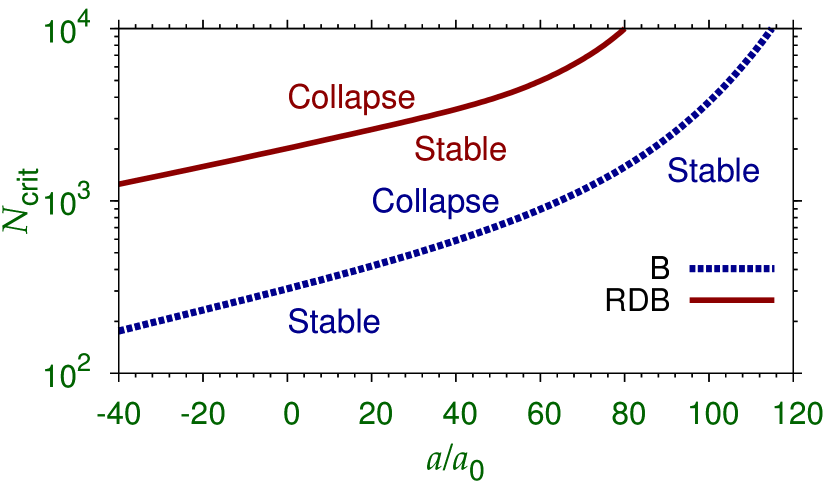
We study the domain of the appearance of the 2D bright solitons of (2). These solitons for a specific scattering length can exist for the number of atoms below a critical number beyond which the system collapses [32]. In figure 1 we plot this critical value versus from imaginary-time simulation. The 2D dipolar RDB solitons, as obtained by real-time simulation, have a much larger spatial extension compared to the bright solitons and can accommodate a larger number of atoms as can be seen from figure 1. For , the soliton collapses due to an excess of dipolar attraction. In the stable region there is a balance between attraction and repulsion to form the bright soliton. The number of atoms in the 2D dipolar bright and RDB solitons could be quite large and will be of experimental interest. The size of quasi-1D nondipolar solitons is usually quite small and accommodates only a small number of atoms.
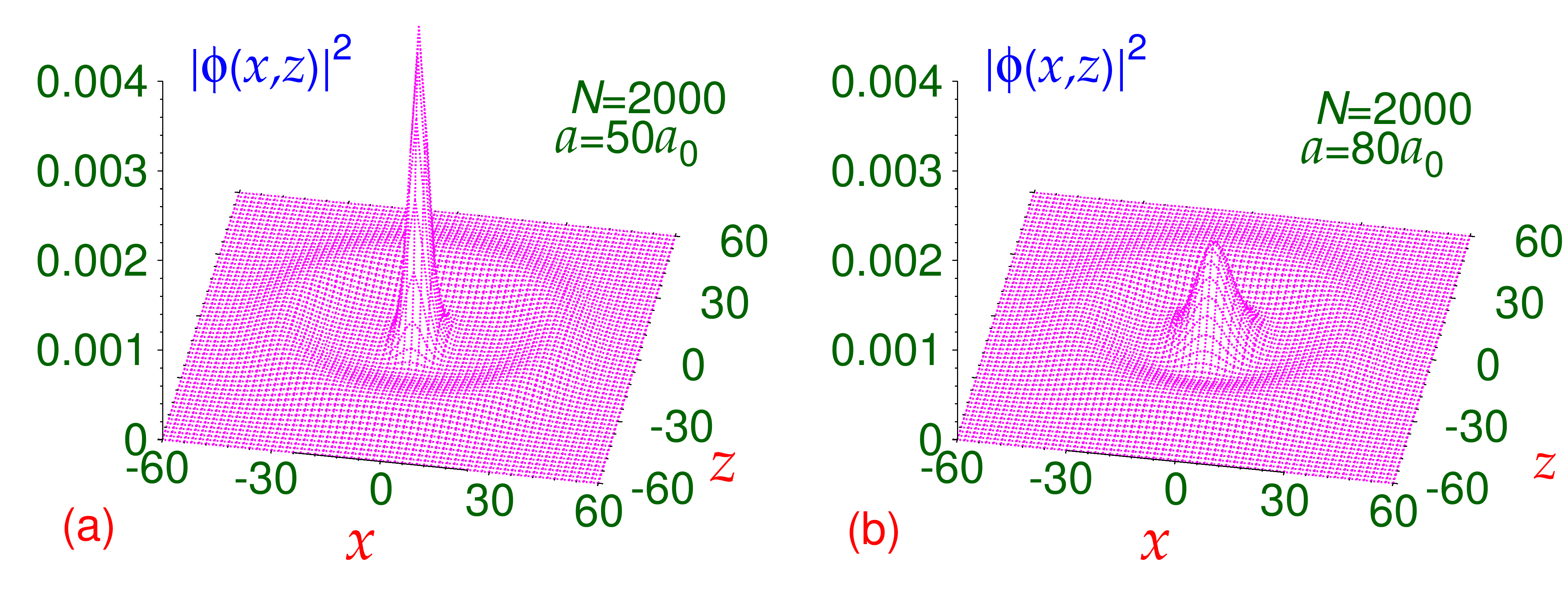
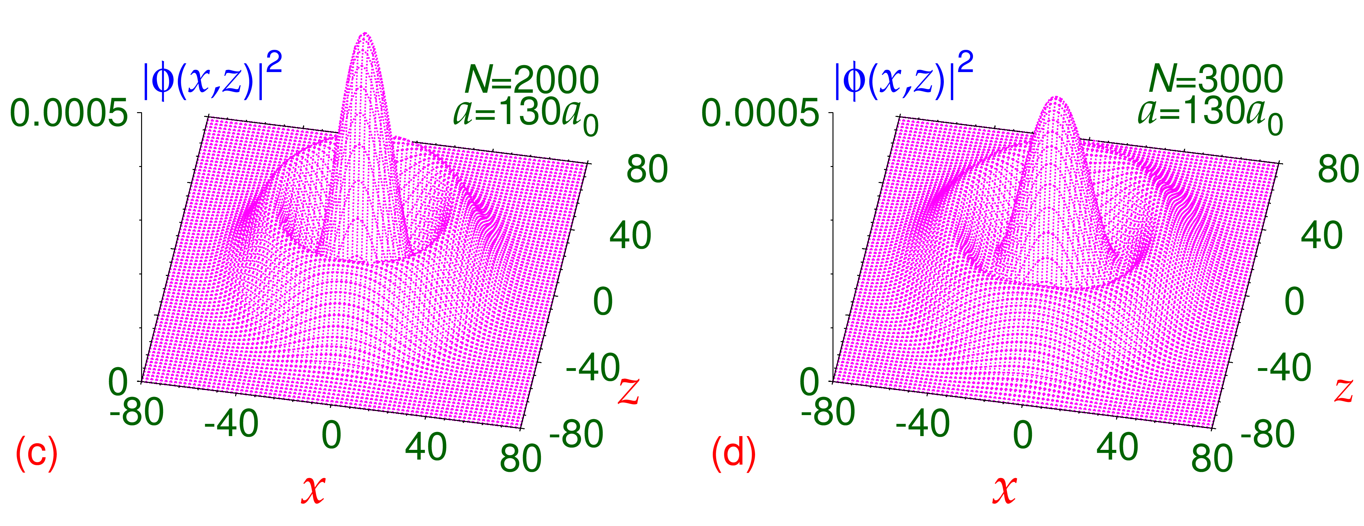
Next we present the profile of the 2D RDB solitons as obtained from (2) by real-time propagation for different number of 164Dy atoms and different scattering lengths. The scattering length can be adjusted to a desired value by the magnetic [33] and optical [34] Feshbach resonance technique. The densities of the different RDB solitons for (a) , (b) , (c) , and (d) , are shown in figure 2. A Gaussian input wave function converges to the 2D bright soliton studied in Ref. [21]. The input functions (7) and (8) in (3) and (2), respectively, with a circular notch at representing a radial excitation, converge to the RDB soliton profiles shown in figure 2. Due to the anisotropic dipolar interaction, the densities of the RDB solitons are anisotropic in the plane when the dipolar interaction dominates the contact interaction (). Although the notch in the density of the RDB soliton can clearly be seen in plots of figure 2, the anisotropic shapes of the densities can be clearly seen in contour plots of densities and this is why we consider the contour plots of density in the following.
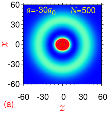
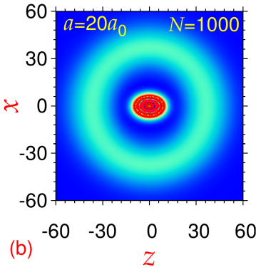
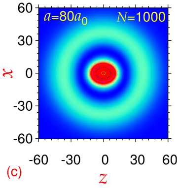
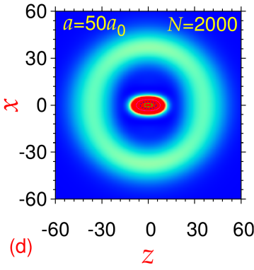
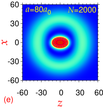
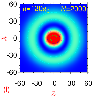
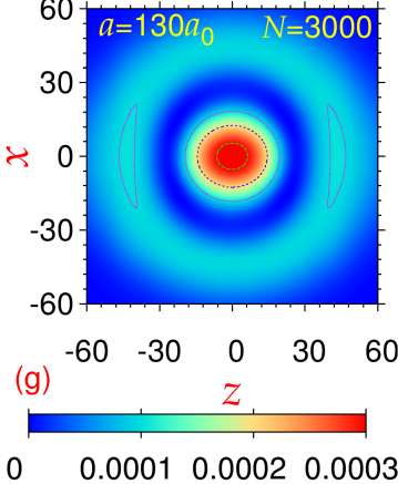
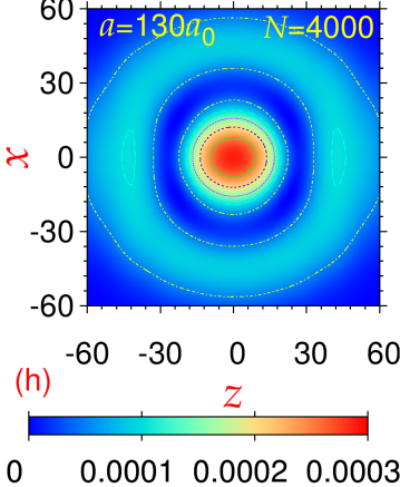
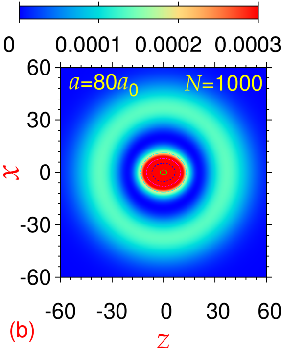
In figure 3 we display the contour plots of the density of 2D RDB solitons for different number of 164Dy atoms and scattering lengths . From figures 2 and 3 and other calculations not presented here, several aspects of the density profiles of the RDB solitons are clear. For a small number of atoms () the dipolar nonlinearity is small and consequently the density profile possesses approximate circular symmetry in the plane. Deviation from circular symmetry occurs for a larger number of atoms and for when the dipolar interaction plays a dominating role in the formation of the RDB solitons. Comparing figures 3(c) and (e) for 1000 and 2000 atoms with scattering length , we see that the anisotropy is larger for a larger number of atoms. Comparing figures 3(d), (e) and (f) for and , respectively, for we find that the anisotropy has reduced with an increase of the scattering length from to . For , the anisotropic dipolar interaction plays a less dominating role in the formation of the RDB soliton and hence results in a reduced anisotropy in figures 3(f), (g) and (h) for and 4000.
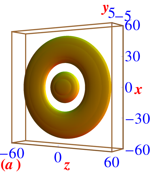
The results reported in this paper are performed with the quasi-2D GP equation (2). Although this seems very reasonable in the presence of a strong trap in the transverse direction, it is worthwhile to compare these densities with those obtained from a solution of the 3D GP equation (3) and we do this in the following. We calculated the density of several of the RDB solitons illustrated in figure 3 using the 3D GP equation (2). The quasi-2D densities obtained from the 2D and 3D GP equations are very similar in all cases. In figure 4(a) we show the 3D Isodensity profile of the RDB soliton obtained from (3) for and . The quasi-2D density obtained from the same calculation is shown in figure 4(b). This quasi-2D density is very similar to the same presented in figure 3(c) from a solution of the quasi-2D GP equation (2), which validates the use of this equation.
The 2D RDB solitons presented in figures 2 and 3 are stable and robust as tested under real-time propagation with a reasonable perturbation in the parameters. The robustness comes from the large contact repulsion which inhibits collapse. Also, the predominant long-range dipolar attraction in the plane prevents the leakage of the atoms to infinity. In a nondipolar quasi-1D BEC soliton, the contact attraction alone provides the binding and there is no repulsion to stop the collapse. We provide below two numerical tests for the stability of a RDB soliton.
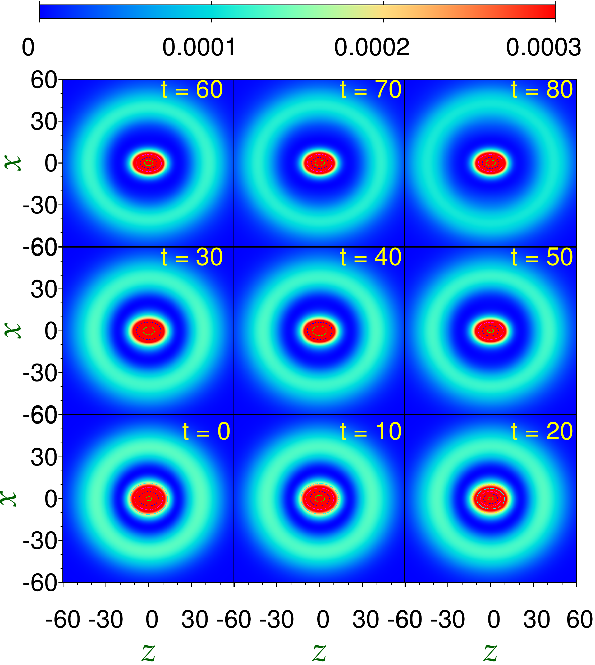
First we test the stability of a RDB soliton under a sudden change of the scattering length. We perform real-time simulation, with the wave function of the RDB soliton of figure 3(c) as the initial state, when at time the scattering length is suddenly changed from to . The contour plots of density at different times is exhibited in Fig, 5. Although the notch in the density remains intact, at large times the RDB soliton adjusts to the shape with shown in figure 3(b). The anisotropy has increased with time due to an increased contribution of dipolar interaction as the contact interaction is reduced at .
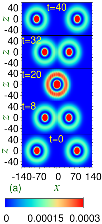
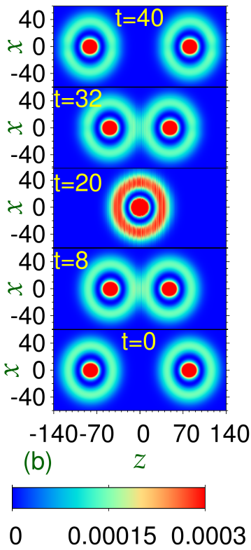
A stringent test of the robustness of these 2D RDB solitons is provided in their behavior under head-on collision. Like the 1D dipolar solitons [20], the collision of the RDB solitons is expected to be quasi elastic with the solitons emerging with little deformation after collision at medium velocities. Only the collision between two integrable 1D solitons is known to be perfectly elastic at all velocities [1]. We consider a head-on collision between two 2D RDB solitons of figure 3(c) moving in opposite directions along both and axes. The collision dynamics of two such solitons as generated from a real-time simulation of Eq. (2) is shown in figure 6(a) and (b), respectively. The initial velocities of the two solitons are attributed by multiplying the initial wave functions of the two solitons by phase factors . The two 2D dipolar RDB solitons are initially placed at and the real-time simulation started. The two solitons move in opposite directions and suffer a head-on collision. The collision dynamics for velocity along direction is illustrated by plotting the density of the system at different times as shown in figure 6(a). The dimensionless velocity of each soliton is about , which corresponds to about 1.5 mm/s using scales m and ms. In figure 6(b) we show the collision dynamics for velocity along direction. The smooth density profiles of the dynamics presented in figure 6 illustrates the quasi elastic nature of the dynamics. In figure 7(a) we plot the final density of one of the solitons after collision at shown in figure 6(b) and compare it with the initial density before collision shown in figure 7(b). The similarity of the two densities shown in figure 7 illustrates the quasi-elastic nature of the collision.
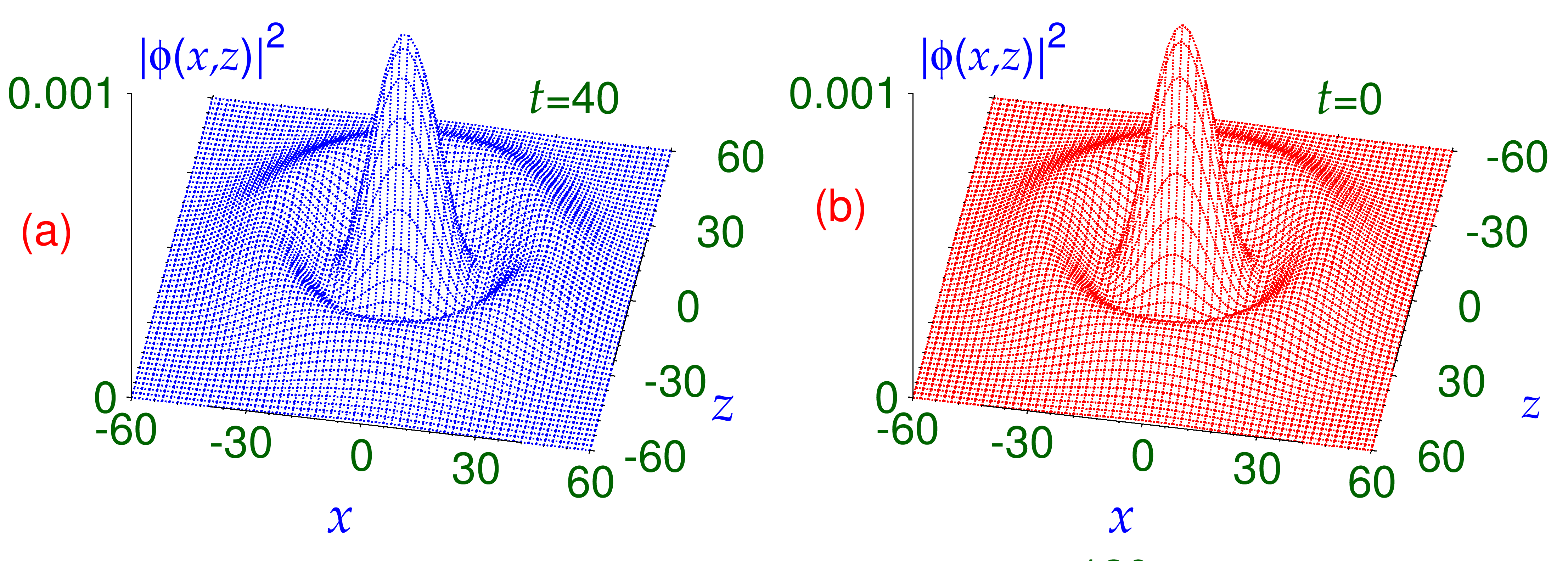
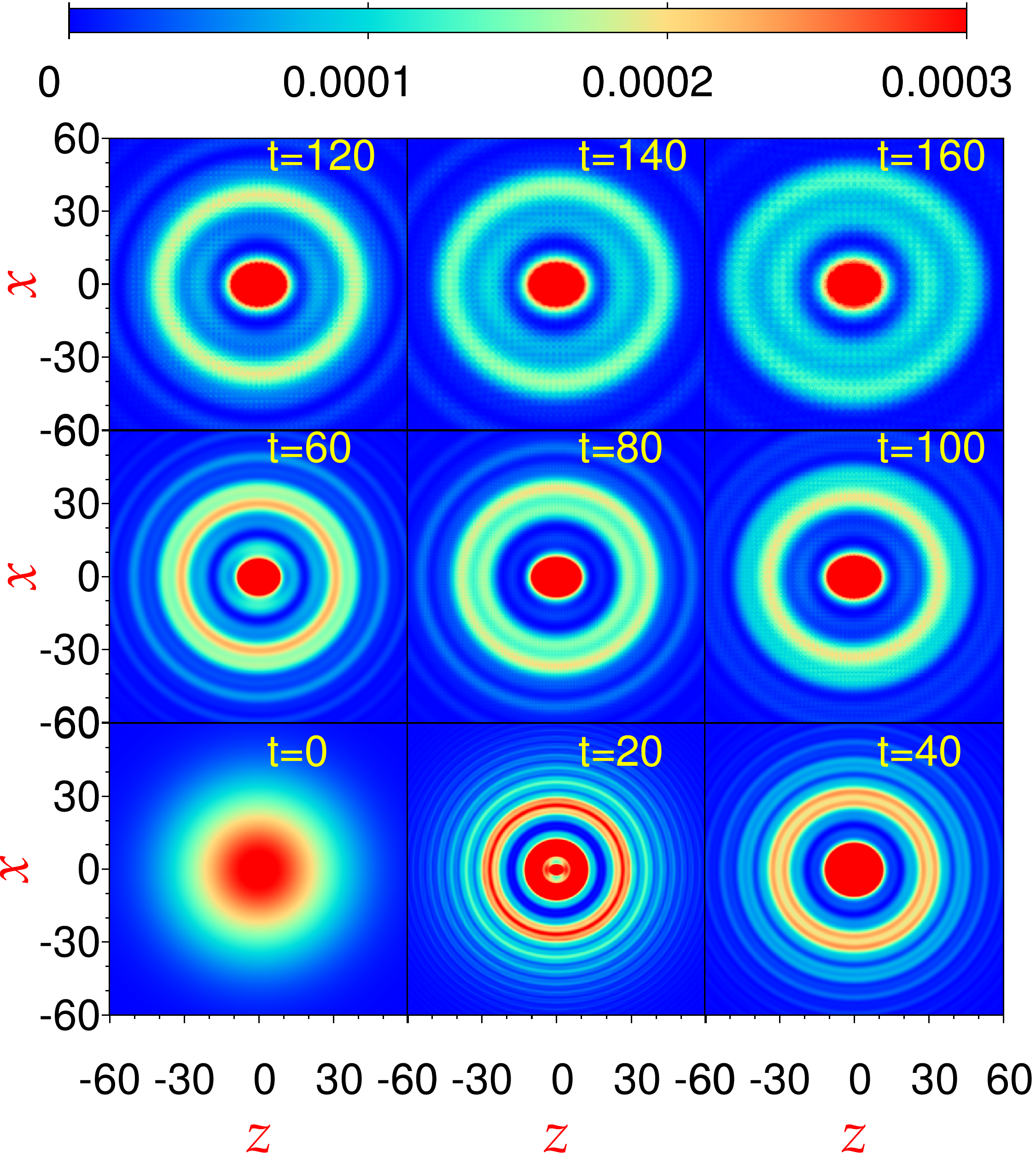
As the 2D dipolar RDB solitons are stable and robust, they can be prepared from the phase-imprinted [26] Gaussian profile
| (9) | |||||
| (10) |
in the trapless case. In an experiment a homogeneous potential generated by the dipole potential of a far detuned laser beam should be applied on part of the Gaussian profile () for an interval of time so as to imprint an extra phase of on the wave function for [4]. The thus phase-imprinted Gaussian profile with is propagated in real-time with and , while it slowly transforms into a 2D dipolar RDB soliton. This simulation is done with no trap. In actual experiment a very weak in-plane trap can be kept during generating the 2D RDB soliton, which can be eventually removed. The simulation is shown in figure 8, where we show the density at different times. It is illustrated that at large times the density evolves towards that of the 2D RDB soliton shown in figure 3(c).
4 Summary
We demonstrated the possibility of creating a mobile, stable 2D RDB soliton, in a dipolar quasi-2D BEC of 164Dy atoms polarized along axis and trapped along axis, with a circular notch and capable of moving in the plane with a constant velocity. The 2D RDB solitons are stationary solutions of the mean-field GP equation. The stability of the RDB soliton is established from a prolonged real-time simulation after a sudden change of the scattering length. The head-on collision between two such solitons with a relative velocity of about 1.5 mm/s is quasi elastic with the solitons passing through each other with practically no deformation. A possible way of preparing these 2D dipolar RDB solitons by phase imprinting a Gaussian profile is demonstrated using real-time propagation. The results and conclusions of this paper can be tested in experiments with present-day know-how and technology and should lead to interesting future investigations.
We thank the Fundação de Amparo à Pesquisa do Estado de São Paulo (Brazil, Project No. 2012/00451-0) and the Conselho Nacional de Desenvolvimento Científico e Tecnológico (Brazil, Project No. 303280/2014-0) for partial support.
References
- [1] Kivshar Y S and Malomed B A 1989 Rev. Mod. Phys. 61 763 Abdullaev F K, Gammal A, Kamchatnov A M and Tomio L 2005 Int. J. Mod. Phys. B 19 3415
- [2] Strecker K E, Partridge G B, Truscott A G and Hulet R G 2002 Nature 417 150 Khaykovich L, Schreck F, Ferrari G, Bourdel T, Cubizolles J, Carr L D, Castin Y and Salomon C 2002 Science 256 1290
- [3] Cornish S L, Thompson S T and Wieman C E 2006 Phys. Rev. Lett.96 170401
- [4] Burger S, Bongs K, Dettmer S, Ertmer W, Sengstock K, Sanpera A, Shlyapnikov G V and Lewenstein M 1999 Phys. Rev. Lett. 83 5198 Dutton Z, Budde M, Slowe C and Hau L V 2001 Science 293 663
- [5] Denschlag J, Simsarian J E, Feder D L, Clark C W, Collins L A, Cubizolles J, Deng L, Hagley E W, Helmerson K, Reinhardt W P, Rolston S L, Schneider B I and Phillips W D 2000 Science 287 97
- [6] Anderson B P, Haljan P C, Regal C A, Feder D L, Collins L A, Clark C W and Cornell E A 2001 Phys. Rev. Lett.86 2926
- [7] Frantzeskakis D J 2010 J. Phys. A: Math. Gen.43 213001 Busch Th and Anglin J R 2000 Phys. Rev. Lett.84 2298 Fedichev P O, Muryshev A E and Shlyapnikov G V 1999 Phys. Rev.A 60 3220
- [8] Muryshev A, Shlyapnikov G V, Ertmer W, Sengstock K and Lewenstein M 2002 Phys. Rev. Lett.89 110401
- [9] Becker C, Stellmer S, Soltan-Panahi P, Dörscher S, Baumert M, Richter E-M, Kronjäger J, Bongs K and Sengstock K 2008 Nature Phys. 4 496 Shomroni I, Lahoud E, Levy S and Steinhauer J 2009 Nature Phys. 5 193
- [10] Feder D L, Pindzola M S, Collins L A, Schneider B I and Clark C W 2000 Phys. Rev.A 62 053606
- [11] Theocharis G et al. 2003 Phys. Rev. Lett.90 120403
- [12] Kivshar Y S and Yang X 1994 Phys. Rev.E 50 R40 Frantzeskakis D J and Malomed B A 1999 Phys. Lett.A 264 179 Zhang J-F, Wu L, Li L, Mihalache D and Malomed B A 2010 Phys. Rev.A 81 023836
- [13] Neshev D, Dreischuh A, Kamenov V, Stefanov I, Dinev S, Fliesser W and Windholz L 1997 Appl. Phys. B 64 429
- [14] Wang W et al. 2015 Phys. Rev.A 92 033611 Hu X-H, Zhang X-F, Zhao D, Luo H-G and Liu W M 2009 Phys. Rev.A 79 023619 Toikka L A and Suominen K-A 2013 Phys. Rev.A 87 043601
- [15] Song S-W, Wang D-S, Wang H and Liu W M 2012 Phys. Rev.A 85 063617
- [16] Lu M, Youn S H and Lev B L 2010 Phys. Rev. Lett.104 063001
- [17] Lu M, Burdick N Q, Youn S H and Lev B L 2011 Phys. Rev. Lett.107 190401
- [18] Aikawa K, Frisch A, Mark M, Baier S, Rietzler A, Grimm R and Ferlaino F 2012 Phys. Rev. Lett.108 210401
- [19] Lahaye T et al. 2007 Nature 448 672 Koch T, Lahaye T, Metz J, Fröhlich B, Griesmaier A and Pfau T 2008 Nature Phys. 4 218
- [20] Young-S L E, Muruganandam P and Adhikari S K 2011 J. Phys. B: At. Mol. Opt. Phys.44 101001
- [21] Nath R, Pedri P and Santos L 2009 Phys. Rev. Lett.102 050401 Tikhonenkov I I, Malomed B A and Vardi A 2008 Phys. Rev. Lett.100 090406 Köberle P, Zajec D, Wunner G and Malomed B A 2012 Phys. Rev.A 85 023630
- [22] Adhikari S K and Muruganandam P 2012 Phys. Lett. A 376 2200
- [23] Adhikari S K and Muruganandam P 2012 J. Phys. B: At. Mol. Opt. Phys.45 045301 Tikhonenkov I, Malomed B A and Vardi A 2008 Phys. Rev.A 78 043614
- [24] Adhikari S K Phys. Rev.A 2014 89 043615
- [25] Adhikari S K 2014 J. Phys. B: At. Mol. Phys.47 225304
- [26] Dobrek L, Gajda M, Lewenstein M, Sengstock K, Birkl G and Ertmer W 1999 Phys. Rev.A 60 R3381
- [27] Lahaye T, Menotti C, Santos L, Lewenstein M and Pfau T 2009 Rep. Prog. Phys. 72 126401
- [28] Kishor Kumar R, Young-S L E, Vudragovic D, Balaz A, Muruganandam P and Adhikari S K 2015 Comput. Phys. Commun. 195 117
- [29] Muruganandam P and Adhikari S K 2012 Laser Phys. 22 813 Fischer U R 2006 Phys. Rev.A 73 031602 Pedri P and Santos L 2005 Phys. Rev. Lett.95 200404
- [30] Muruganandam P and Adhikari S K 2009 Comput. Phys. Commun. 180 1888 Vudragović D, Vidanovic I, Balaž A, Muruganandam P and Adhikari S K 2012 Comput. Phys. Commun. 183 2021
- [31] Goral K and Santos L 2002 Phys. Rev.A. 66 023613
- [32] Ronen S, Bortolotti D C E and Bohn J L 2007 Phys. Rev. Lett.98 030406
- [33] Inouye S et al. 1998 Nature 392 151
- [34] Fedichev P O, Kagan Yu, Shlyapnikov G V and Walraven J T M 1996 Phys. Rev. Lett.77 2913