History effects in the sedimentation of light aerosols in turbulence: the case of marine snow

Abstract

We analyze the effect of the Basset history force on the sedimentation of nearly neutrally buoyant particles, exemplified by marine snow, in a three-dimensional turbulent flow. Particles are characterized by Stokes numbers much smaller than unity, and still water settling velocities, measured in units of the Kolmogorov velocity, of order one. The presence of the history force in the Maxey-Riley equation leads to individual trajectories which differ strongly from the dynamics of both inertial particles without this force, and ideal settling tracers. When considering, however, a large ensemble of particles, the statistical properties of all three dynamics become more similar. The main effect of the history force is a rather slow, power-law type convergence to an asymptotic settling velocity of the center of mass, which is found numerically to be the settling velocity in still fluid. The spatial extension of the ensemble grows diffusively after an initial ballistic growth lasting up to ca. one large eddy turnover time. We demonstrate that the settling of the center of mass for such light aggregates is best approximated by the settling dynamics in still fluid found with the history force, on top of which fluctuations appear which follow very closely those of the turbulent velocity field.

I Introduction

There is an increasing evidence, both theoretical and experimental, pointing out the relevance of memory effects in the advection of inertial particles (see e.g. Tanga and Provenzale (1994); Belmonte et al. (2001); Daitche and Tél (2011); Guseva et al. (2013); Daitche and Tél (2014); Farazmand and Haller (2015); Mordant and Pinton (2000); Candelier et al. (2004); Vojir and Michaelides (1994); Langlois et al. (2015)). Several further studies concerning these effects in turbulence are reviewed in Daitche (2015). The equations of motion for small spherical inertial particles were formulated by Maxey and Riley Maxey and Riley (1983) and Gatignol Gatignol (1983) with corrections by Auton et al. Auton et al. (1988) and are of integro-differential type in their full form. They contain an integral term which accounts for the diffusion of vorticity around the particle throughout its entire history. This integral term is called the history (or Basset) force Basset (1888), and it has become clear by now that the often used approximation in which this term is neglected is improper, and the full Maxey-Riley equation should be considered  Tanga and Provenzale (1994); Belmonte et al. (2001); Daitche and Tél (2011); Guseva et al. (2013); Daitche and Tél (2014); Farazmand and Haller (2015); Langlois et al. (2015); Mordant and Pinton (2000); Candelier et al. (2004); Daitche and Tél (2011); van Hinsberg et al. (2011); Vojir and Michaelides (1994); Daitche (2013, 2015).

In this work, we analyze the effect of the history force on sedimenting particles in turbulence in the presence of gravity. Previous efforts to understand the importance of the history force in the presence of gravity in smooth flows are due to Mordant and Pinton Mordant and Pinton (2000) and to Lohse and coworkers Toegel et al. (2006); Garbin et al. (2009) who also carried out experiments. Their studies, however, concentrated on free sedimentation, that is on the particle motion in a fluid at rest, and on bubble dynamics in a standing wave, respectively. More recent papers investigate the problem in a stationary Bergougnoux et al. (2014) and periodically changing cellular flow Guseva et al. (2013). The sedimentation problem in turbulent flows is considered up to now – to our knowledge – only in stratified turbulence Aartrijk and Clercx (2010) and for the plankton problem Olivieri (2013).

The motivation for our particular range of parameters comes from recent studies of marine ecosystems which emphasize the importance of marine snow. Marine snow plays a central role in the carbon cycle Mann and Lazier (2005); De La Rocha and Passow (2007); Riley et al. (2012), and its formation is mainly due to physical aggregation, a consequence of particle-flow interactions. Sedimentation of marine snow is considered to account for a large fraction of carbon sequestration into the deep ocean Stone (2010); Passow and Carlson (2012) this net ocean sequestration flux is estimated to reach $\sim 10^{15}\;g\;Carbon/yr$ Passow and Carlson (2012). The physical and biological properties of marine snow aggregates make it rather difficult to estimate their sinking velocity. The techniques employed to evaluate settling velocities vary across different measurements McDonnell and Buesseler (2010); Petrik et al. (2013), and the results are difficult to compare due to the variation in density and sizes of the used aggregates. An additional difficulty for in situ experiments is the fact that turbulent kinetic energy varies with depth Gargett (1989). While some laboratory experiments with grid generated turbulence Murray (1970); Tooby et al. (1977) and in situ measurements Alldredge and Gotschalk (1988) find indications for a retarded settling in situ compared to laboratory measurements in still water, other observations in coastal areas Shanks (2002) and in the laboratory using Couette devices Ruiz et al. (2004) report an enhancement of the sinking speed in turbulence.

Marine snow particles contain organic and inorganic components as primary particles which stick together in a fractal-like structure possessing a relatively high porosity. This fact has been taken into account in concepts working with an effective density  Kranenburg (1994); Winterwerp (1998), an effective diameter Logan and Wilkinson (1990) or a modified Stokes law Khelifa and Hill (2006) of the aggregates. Moreover, sinking marine aggregates undergo changes in size and density due to aggregation and fragmentation processes influencing the settling of them  Jackson et al. (2005).

Those biological properties are difficult to take into account when modeling the sinking of marine aggregates as inertial particles using the Maxey-Riley equation. The fractal shape can be taken into account by means of an effective density Zahnow et al. (2011), but this has been studied so far only neglecting the history force. Since the latter has not yet been formulated for more complicated objects than spheres, the study presented here will work exclusively with spherical particles the properties of which are based on the effective aggregate diameters and effective densities given in the literature. The effective densities of marine aggregates are usually very close to the water density and a general property is that larger aggregates have smaller density than small ones. The relationship between the size (average effective radius $a$) and effective excess density $\Delta\rho$ between particle and fluid ($\Delta\rho=\rho_{p}-\rho_{f}$) for aggregates rich in biological components was proposed by McCave et al McCave (1984) to be $\Delta\rho\propto a^{-1.3}$ , and this relation was used to fit the experimental results Tambo and Watanabe (1979), see middle curve in Fig. 1. This relation is close to the one obtained from in situ measurements from Santa Barbara Channel by Alldredge et al Alldredge and Gotschalk (1988), $\Delta\rho\propto a^{-1.6}$ for marine snow characterized by $a>250\;\mu m$, also with predominately organic composition (lowest curve Fig. 1). On the other hand, in estuaries and coastal regions aggregate composition includes more inorganic components  Simon et al. (2002), therefore, they are smaller and slightly denser than the ones formed in the ocean. The corresponding effective size effective density relationship was studied by Soulsby et al Soulsby et al. (2013), and assumes $\Delta\rho\propto a^{-0.66}$ (see uppermost curve in Fig. 1). For a review see Winterwerp (2011). Typical velocities in the ocean’s upper layer are strongly dependent on the wind and can reach up to $0.5$ m$/$s Oakey and Elliott (1982). The turbulent kinetic energy $\epsilon$ typical for the open ocean is $\epsilon=10^{-6}$ m${}^{2}/$s³ Mann and Lazier (2005); Kirboe and Saiz (1995), which sets the size of the smallest possible eddies, the Kolmogorov length $\eta$ to be $\sim 10^{-3}$ m. The size of aggregates (macroaggregates) varies from $0.1$ to less than $1$ mm De La Rocha and Passow (2007); Bartholomä et al. (2009), however the average aggregate size is always at most $\eta/2$ according to  De La Rocha and Passow (2007); Bartholomä et al. (2009), though the relationship between the average aggregate size and the turbulent kinetic energy in the ocean is not well established due to the difficulty of in situ measurements.

Since we are interested in the effect of the history force we are confined to a certain, yet realistic, set of parameters for size and density of our marine snow particles which maximize the impact of the history force. On the one hand we need Stokes numbers that are not too small for the history term to play an important role. On the other hand, having a small Stokes number also decreases the impact of preferential concentrations. To study the problem, we select six density-size pairs typical of marine snow. The radii are 0.5 and 0.3 mm, since the strongest impact of the history force is expected at the largest sizes, largest possible Stokes numbers Daitche (2015). To both of these sizes we assign three different densities, see Fig 1. We also display the results of the relationship of the excess density $\Delta\rho$ and particle diameter $a$ for open ocean Soulsby et al. (2013) and coastal areas McCave (1984). The sizes and the flow set the Stokes numbers (see Eq.(6) below) which take the values $St=0.083$ and $St=0.03$, respectively. The parameters characterizing the six cases are summarized in Table I.

case	$\Delta\rho$ (g/cm3)	$\beta$	$a$ (m)	$St$	$W$	$Re_{z}^{*}$
(I)	0.015	0.9900			8.21	4.1
(II)	0.0075	0.9950	$5\cdot 10^{-4}$	0.083	4.12	2
(III)	0.003	0.9980			1.65	0.8
(IV)	0.05	0.9677			9.67	2.9
(V)	0.025	0.9836	$3\cdot 10^{-4}$	0.03	4.91	1.5
(VI)	0.01	0.9934			1.98	0.6

Table 1: Parameters for six representative cases of marine aggregates in the ocean ((I), (II), (III)) and coastal areas ((IV), (V), (VI)). Parameters $\beta$, $St$, $W$ and $Re^{*}_{z}$ are defined in equations (5), (6), (7), and (1), respectively, and turbulence data are taken from Table II.

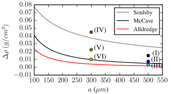
Figure 1: Representation of the chosen parameters (see Table I) on the particle radius–excess density plane. The two lower curves represent the relationship between the effective excess density $\Delta\rho$ and the effective radius $a$ for aggregates with predominantly organic composition McCave (1984); Alldredge and Gotschalk (1988), as expeceted for the open ocean, while the uppermost curve shows this relationship for aggregates from coastal areas and estuaries Soulsby et al. (2013), containing a large fraction of inorganic components.

As a preliminary qualitative analysis, let us concentrate here on the particle Reynolds number $Re_{p}$ that should not exceed a limit. It should be below or of the order of unity for the Stokesian drag to be valid, at least in a good approximation. Since gravity breaks the isotropy of the advection problem by preferring the vertical ($z$) direction, and particles are nearly neutrally bouyant, it is worth defining a vertical and a horizontal particle Reynolds number for spheres of radius $a$ and of typical slip velocity $\vec{v}-\vec{u}$ relative to the fluid

$$Re_{z}^{*}=\frac{a|v_{z}-u_{z}|}{\nu},\qquad Re_{h}^{*}=\frac{a|\vec{v_{h}}-\vec{u_{h}}|}{\nu},$$ (1)

where index $h$ refers to the horizontal component, and $\nu$ is the fluid’s kinematic viscosity. The corresponding usual particle Reynolds number $Re_{p}$ follows from the identity $Re_{p}^{2}=Re_{z}^{2}+Re_{h}^{2}$. The order of magnitude of the vertical slip velocity is the settling velocity in still water which we write as $W_{\text{settling}}=Wu_{\eta}$, where $W$ is the dimensionless settling velocity taken in units of the Kolmogorov velocity $u_{\eta}$ (all results for turbulent advection will be given in Kolmogorov units). Measuring the particle radius in Kolmogorov length, $\eta$, we find

$$Re_{z}^{*}=\frac{a}{\eta}\frac{Wu_{\eta}\eta}{\nu}=W\frac{a}{\eta},$$ (2)

since the fluid Reynolds number on the Kolmogorov scale $u_{\eta}\eta/\nu$ is by definition unity. The horizontal slip velocity is expected to vanish with the Stokes number. Therefore, the horizontal slip velocity should be proportional to $Stu_{\eta}$. Taking the proportionality factor to be unity, we find for the horizontal Reynolds number in an analogous manner the estimate

$$Re_{h}^{*}=St\frac{a}{\eta}.$$ (3)

Since $St\ll W$ (see Table I.), we find that $Re_{p}\approx Re_{z}$. We think that this is a central property of marine snow sedimentation, which expresses that these particles behave horizontally as nearly neutrally bouyant, but they sediment with a speed comparable to that of the small scale fluctuations of the fluid ($u_{\eta}$), i.e. they are not neutrally bouyant from the point of view of the vertical dynamics. We shall in fact see that the instantaneous particle Reynolds numbers converge in time towards $Re_{z}^{*}$. The characteristic numbers $Re^{*}_{z}$ are also indicated in Table I.

The paper is organized as follows: In Sec. II we present an overview of the equation of motion with the history force. Next, we recall an infinite series solution of it in still fluid and find a simple analytic approximation to be valid after relatively short times, presented in Sec. III. Then we summarize the approach used to compute the history force, and to generate the turbulent velocity field in Sections IV. In Sec. V our numerical results concerning the sedimentation dynamics in space are summarized. In section VI we turn to results on velocities and accelerations. Sec. VII is devoted to estimating the relevance of the Faxén corrections. Our final conclusions are given in Sec. VIII.

II Equation of motion and notations

We analyze the advection of spherical, rigid particles with a small particle Reynolds number in an incompressible and viscous fluid. The Lagrangian trajectories of such particles are evaluated according to the Maxey-Riley equation Maxey and Riley (1983); Gatignol (1983), including the corrections by Auton and coworkers Auton et al. (1988). In the full Maxey-Riley picture one describes the dimensionless evolution of the particle position $\vec{x}(t)$ and velocity $\vec{v}(t)=d\vec{x}/dt$ in a flow field $\vec{u}(\vec{x},t)$. Without Faxén corrections the equation of motion reads as

$$\frac{d\vec{v}}{dt}=\frac{1}{St}(\vec{u}-\vec{v})+\frac{W}{St}\vec{n}+\beta\frac{D\vec{u}}{Dt}-\sqrt{\frac{3\beta}{\pi St}}\int_{0}^{t}\frac{\frac{d(\vec{v}-\vec{u})}{d\tau}}{\sqrt{t-\tau}}d\tau,$$ (4)

where $\vec{n}$ is the vertical unit vector pointing downwards. This form of the equation holds when the particle is initialized at time zero with a velocity coinciding with that of the fluid, zero initial slip velocity. We have to distinguish the full derivative along a fluid element and a particle trajectory, given by

$$\frac{D}{Dt}=\frac{\partial}{\partial t}+\vec{u}\cdot\nabla\qquad\text{and}\qquad\frac{d}{dt}=\frac{\partial}{\partial t}+\vec{v}\cdot\nabla,$$

respectively. The velocity of the particle changes due to the action of different forces. The forces in (4) represent from left to right: the Stokes drag, the gravity, the pressure force (which accounts for the force felt by a fluid element together with the added mass force), and lastly the Basset history force. The equation is written in dimensionless form, rescaled by the Kolmogorov time $\tau$ and the Kolmogorov length scale $\eta$ of the flow ($u_{\eta}=\eta/\tau_{\eta})$. The ratio

$$\beta=\frac{3\rho_{f}}{\rho_{f}+2\rho_{p}}=\frac{3\rho_{f}}{3\rho_{f}+2\Delta\rho}$$ (5)

characterizes the excess density of the particle $\Delta\rho$ and the density of the fluid $\rho_{f}$. For aerosols $\beta<1$ .

Another dimensionless parameter in Eq. (4) is the Stokes number

$$St=\frac{a^{2}}{3\nu\beta\tau_{\eta}}=\frac{\tau_{p}}{\tau_{\eta}},$$ (6)

which is the ratio of the particles’ relaxation time $\tau_{p}$ due to kinematic viscosity $\nu$ of the fluid to the Kolmogorov time.

Additionally, parameter $W$ governs the dimensionless settling velocity in still fluid. It can be written as

$$W=St(\beta-1)\frac{g\eta}{u^{2}_{\eta}},$$ (7)

where the last factor corresponds to the reciprocal of a turbulent Froude number. It is to be emphasized that $W$ cannot be varied freely: an ad-hoc choice of $W$ to a given $St$ could imply that, for a fixed density, the flow and/or the gravity $g$ are changed. The $W$ values given in Table I., used by us, are the ones which follow from the particle properties and the characteristics of our turbulent flow. Anyhow, in sedimentation the role of the dimensionless settling velocity might be more relevant than that of the Stokes number.

We shall compare the Maxey-Riley equation (Eq.(4)) to the approximation which does not take into account the history force,

$$\frac{d\vec{v}}{dt}=\frac{1}{St}(\vec{u}-\vec{v}+W\vec{n})+\beta\frac{D\vec{u}}{Dt},$$ (8)

often called the advective equation of inertial particles. We emphasize that Eq.(8) does not follow from any approximation of the Maxey-Riley equation for our sets of particle parameters, its use is motivated by mere numerical convenience.

We also carry out simulations with the equation

$$\vec{v}=\vec{u}+W\vec{n},$$ (9)

valid for ideal non-inertial particles. Note that this case arises when $St\rightarrow 0$, and is the limit of both equations (4) and (8), with different convergence properties, of course.

III Settling in still fluid

The exact solution for the settling in a still fluid $(\vec{u}=0)$ was worked out by Belmonte and coworkers Belmonte et al. (2001). In this case a natural velocity unit is the settling velocity $W_{\text{settling}}$, and time can be measured in units of the particle relaxation time $\tau_{p}$. In these units, the dimensionless vertical velocity $v^{\prime}_{z}(t^{\prime})$ in dimensionless time $t^{\prime}$ can be expressed in terms of complementary error functions $erfc$. With zero initial velocity it reads in our notation as

$$v^{\prime}_{z}(t^{\prime})=1+\frac{\sqrt{3}\beta}{\alpha_{1}-\alpha_{2}}\bigg{[}\frac{e^{\alpha_{1}t^{\prime}}\text{Erfc}\left(\sqrt{\alpha_{1}t^{\prime}}\right)}{\sqrt{\alpha_{1}}}\\ -\frac{e^{\alpha_{2}t^{\prime}}\text{Erfc}\left(\sqrt{\alpha_{2}t^{\prime}}\right)}{\sqrt{\alpha_{2}}}\bigg{]}$$ (10)

where $\alpha_{1}$, $\alpha_{2}$ are the roots of the quadratic equation $\alpha^{2}+(2-3\beta)\alpha+1=0$ depending only on the density via parameter $\beta$.

By keeping only the leading terms of the power law expansion of the function $e^{u}$Erfc$(\sqrt{u})$ for large $u$ (long times $t^{\prime}$), we find

$$v^{\prime}_{z}(t^{\prime})=1-\sqrt{\frac{3\beta}{\pi t^{\prime}}}\left(1-\frac{(3\beta-2)}{2t^{\prime}}\right).$$ (11)

This form turns out to provide a rather accurate approximation for $t^{\prime}>2$, and even by neglecting the second term in the parenthesis it is very close to the exact solution for $t^{\prime}>22$. Note that these forms do not depend on the particle size since Stokes numbers can only be defined in a moving fluid. Whether the particle Reynolds number $Re_{p}$ remains small, i.e. whether equation (4) remains valid during the entire free fall, should be checked a posteriori in the knowledge of the dimensional settling velocity, the particle size and the fluid’s kinematic viscosity.

For comparison, we mention that the solution of the widely used inertial dynamics equation (Eq.(8)) provides for the same problem a linear differential equation whose solution is with the same zero initial condition, and in the same units:

$$v^{\prime}_{z}(t^{\prime})=1-e^{-t^{\prime}}.$$ (12)

This solution is of completely different character.

The solution of the ideal tracer problem (Eq.(9)) is that the particle velocity jumps immediately from $0$ to unity and remains there forever. Note that this behavior follows from both formulas (11) and (12) in the limit of $\tau_{p}\rightarrow 0$, which is equivalent to taking $t^{\prime}\rightarrow\infty$ in these expressions. Eq. (12), however, does not follow as any limit of (10). Fig. 2 provides a comparison of these different dynamics.

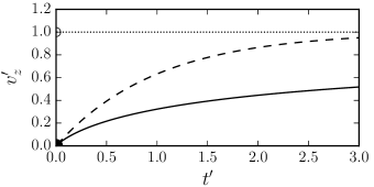
Figure 2: Short-term behavior of the settling in still fluid ($\vec{u}=0$) in the different dynamics investigated. With memory (10): continuous line; without memory (12): dashed line, and non-inertial particles ($v^{\prime}_{z}=1$ for $t^{\prime}>0$, as follows from (9)): dotted line. Note the rather different velocities predicted for any time instant. Time and velocity are measured in units of $\tau_{p}$ and $W_{\text{settling}}$, respectively.

$Re_{\lambda}$	$L_{{\rm box}}/\eta$	$L/\eta$	$\lambda/\eta$	$\Delta x/\eta$	$T_{\mathrm{sim}}/\tau_{\eta}$	$T/\tau_{\eta}$	$\Delta t/\tau_{\eta}$	$u_{\mathrm{rms}}/u_{\eta}$	$N^{3}$
$112$	$633$	$156$	$20.9$	$1.24$	$1020$	$29.0$	$0.015$	$5.39$	$512^{3}$

Table 2: Parameters of the simulated turbulent flow: Taylor Reynolds number $Re_{\lambda}=\lambda u_{\mathrm{rms}}/\nu$, size of the periodic box $L_{{\rm box}}$, integral scale $L=u_{\mathrm{rms}}^{3}/\epsilon$, Taylor microscale $\lambda=u_{\mathrm{rms}}\sqrt{15\nu/\epsilon}$, size of a grid cell $\Delta x$, length of the whole simulation $T_{\mathrm{sim}}$, large-eddy turnover time $T=L/u_{\mathrm{rms}}$, time step $\Delta t$, root-mean-square of the velocity $u_{\mathrm{rms}}=\sqrt{\left\langle\vec{u}^{2}\right\rangle/3}$, number of grid points $N^{3}$. All dimensional quantities are given in multiples of the corresponding Kolmogorov units.

IV Turbulent flow and numerical Simulation

We consider here the case of particles moving in statistically homogeneous, isotropic and stationary turbulence Pope (2000). To this end we solve the vorticity equation, which is equivalent to the incompressible Naiver-Stokes equation, on a grid in a triply-periodic box of size $L_{box}$. The energy is injected by a large scale forcing, see Daitche (2015). For the integration of the flow we use a standard dealiased Fourier-pseudo-spectral method Canuto et al. (1987); Hou and Li (2007) with a third-order Runge-Kutta time-stepping scheme Shu and Osher (1988). The values of Eulerian quantities, which are available on a grid, are obtained at the particle positions through tricubic interpolation. The characteristics of the turbulent flow and the simulation parameters are depicted in Table 2. Since the Kolmogorov scale is $\eta=(\nu^{3}/\epsilon)^{1/4}$ Pope (2000), a fixed value of it can belong to any kinematic viscosity $\nu$ and mean energy dissipation $\epsilon$, as long as the ratio $\nu^{3}/\epsilon$ is fixed. For the particular choice of $\eta=1$ mm, which we shall take as a typical value in our estimations, one finds with the viscosity of water $\epsilon\sim 10^{-6}$ m${}^{2}/$s³.

The presence of the history integral in (4) leads to two problems from the numerical point of view. First, the singularity of the history kernel impedes an accurate numerical solution. This problem can be solved by the use of a specialized integration scheme Daitche (2013) which treats the history force appropriately. This third order scheme has been adjusted for our purposes, see Daitche (2015) for details. Second, it is necessary to recompute the history integral for every new time step. This leads to high computational costs and a high demand for memory (to store the history of each particle). This second problem is inherent to the dynamics with memory and, as a consequence, limits us to a moderate number of particles. For each case of particle parameters we simulated $N_{p}=1.5\cdot 10^{5}$ particles. The initial particle positions have been chosen randomly and homogeneously distributed in the triple-periodic box of size $L_{box}$ of the simulation; the initial particle velocity is that of the fluid at the particle’s position.

V Turbulence: Results on the position of particles

We start by comparing individual trajectories in the Maxey-Riley equation (4), in the inertial equation (8) in which memory is neglected and in the non-inertial dynamics (9). Throughout the paper we will use the following notation for particles following the different dynamical equations (4), (8), and (9), and show their corresponding curves with particular line types:

• particles with memory, continuous line, computed by (4),

• particles without memory, dashed line computed by (8), and

• non-inertial particle, dotted line, computed by (9),

respectively.

Trajectories with the same initial condition, but following these three distinct dynamics, deviate from each other already after a short period of time. The distance among these trajectories increases significantly with time in both the horizontal and the vertical directions. This results in strong differences in the predictions for the position of a particle, since the trajectories of different dynamics can be thousand Kolmogorov lengths away from each other after $500\tau_{\eta}$ as Fig. 3a,d illustrates .

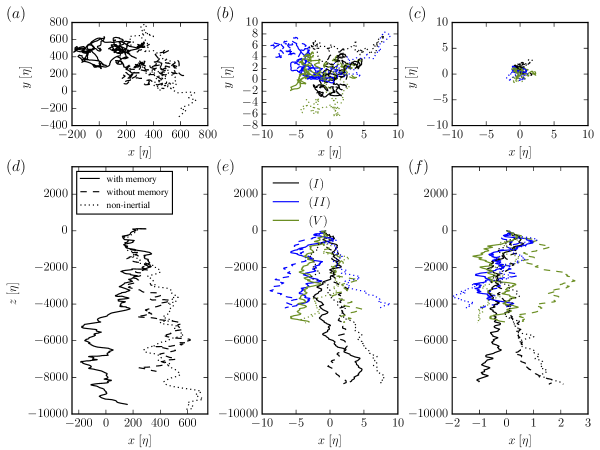
Figure 3: (left) Individual trajectories of the same particle started with the same initial conditions (with zero slip velocity) with the parameter set of case (I), however, following three distinct equations of motion ($x_{0}=293.16\;\eta$, $y_{0}=214.18\;\eta$, $z_{0}=105.71\;\eta$). (middle and right) Position of the center of mass of the ensemble containing $10\%$ of our standard particle number ($N_{p}=1.5\cdot 10^{4}$), and the standard number $N_{p}=1.5\cdot 10^{5}$ of particles, respectively, for the case (I), (II), and (V) evolved with the different equations of motion up to $1020\;\tau_{\eta}$. Here and in the following figures we use the convention that x and t denote the dimensional space and time, respectively, and the dimensions are given in parentheses.

Although there are strong differences for the predictions of the position of an individual particle for these three dynamics Fig. 3d, these differences are smaller when an ensemble is considered Fig. 3e,f. For this analysis we initialize clouds of particles, one with smaller and other with larger number of particles, with the initial condition mentioned above, and evolve them according to our three possible dynamics. The center of mass of each cloud also follows a distinct trajectory, however the distances among the centers of mass do not grow as fast as that of the trajectories of individual particles, see Fig. 3b,c where the final horizontal difference is of a few Kolmogorov lengths only. Moreover, in the $x,y$ planes (upper panels a–c), it becomes clear that the total displacements are in rather different directions with the different dynamics. The horizontal distances between the centers of mass decrease with the number of particles, which can be considered as a consequence of the law of large numbers. The total horizontal displacement in all three dynamics is therefore expected to be zero in the large particle number limit .

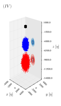
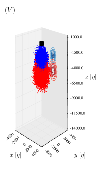
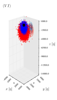
Figure 4: Spatial distribution of the sedimenting particle ensembles for cases (IV), (V) and (VI) simulated with the Maxey-Riley equation (4). Black, blue, and red dots represent the location of the particles at times $t=0$, $510\;\tau_{\eta}$, and $1020\;\tau_{\eta}$, respectively. A 2D histogram of the particle density is projected onto the $(y,z)$ plane, curves represent isolines of densities.

After having seen the results for the center of mass of the particle ensembles, we show in Fig. 4 their distribution in space at three different time instants. It is clear that with large settling velocities the ensemble blobs are well separated after 500 time units, this separation decreases, however, with $W$, and with the smallest settling velocity there is hardly any separation, the blobs strongly overlap, and some points are even above the cube of initial conditions after 1020 time units. These results are obtained in the presence of memory effects but we generated the corresponding figures without memory and with non-inertial particles (governed by Eqs.(8) and (9), respectively), too. No difference can be recognized by naked eyes. This is the first hint to the fact that inspite of the difference in the individual and in the center of mass trajectories following from the different dynamics, the statistical properties are quite similar. To see the differences, more quantitative methods should be taken.

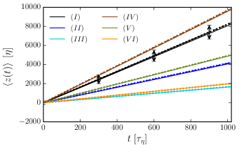
Figure 5: Time-dependence of the $z$-coordinate of the center of mass in the different dynamics, distinguished by different line types, and for all six cases distinguished by different colors, dashed and dotted lines are hard to distinguished in this representation. The two-sided arrows indicate the typical spatial extension in $z$ dimensions of the ensemble for case (I) at the given instances.

In Figure 5 we present a time-continuous plot of the $z$-coordinate of the center of mass for the different cases with the three different dynamics. Here differences become visible, and are on the order of a few hundred Kolmogorov lengths at the end of the simulation. The difference is, however, never larger than a few percent of the instantaneous value of $\left<z\right>$. The long-term behavior is a roughly linear increase in all cases, indicating a rather uniform settling. Note that the graphs for the largest excess density (case (I) and (IV)) are close to each other in spite of the different Stokes numbers. The cases with intermediate and small excess densities behave also similarly.

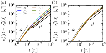
Figure 6: Time-dependence of the variances in the horizontal ($x$, left panel) and vertical ($z$ right panel) directions in the different cases (coloring and line types as in as in the previous figure) on log-log scales. For clarity, the initial variance $\sigma_{x}(0)$ ($=633/\sqrt{12}=183$ in dimensionless units) is subtracted. The graphs of different dynamics are overlaid and dashed and dotted lines are hard to distinguished in this representation. The thin continuous black lines have slopes $2$ and $1$, respectively, to guide the eye.

As seen from Fig. 4, the blob sizes are also important. To monitor their time evolution, we determined the standard deviation $\sigma$ about the center of mass in the horizontal $x$ direction, and in the vertical direction, as Fig. 6 shows. The horizontal and the vertical behavior are different, reflecting again that gravity prefers a certain direction. In fact, the vertical extension of all the blobs is larger than the horizontal one at any instant. The data are plotted on a log-log scale to enlighten the appearance of power law behavior. The two black straight lines represent ballistic ($\sigma^{2}\sim t^{2}$) and diffusive ($\sigma^{2}\sim t$) spreading. A crossover to the diffusive behavior can be observed at $t\sim 20-30$ time units. It is natural to understand that when the blobs are large, the ensembles become subjected to a diffusive spreading by wandering in-between the largest scale vortices.

In order to explain the ballistic behavior, we recall the theory of Batchelor Batchelor (1950) for the separation of pairs of ideal tracers in three-dimensional homogeneous isotropic turbulence. This theory claims that the mean square separation should grow as $t^{2}$ for times shorter than a characteristic time $t_{0}$. For times larger than $t_{0}$ the famous Richardson scaling Pope (2000) should hold characterized by a scaling proportional to $t^{3}$. This regimes extends, however, only up to the time when the effect of the largest coherent structures becomes dominant, i.e. up to the eddy turnover time $T$. The characteristic time $t_{0}$ depends on the initial spatial separation $\vec{r}_{0}$ between the two particles. In dimensional units $t_{0}=(\mid\vec{r}_{0}\mid^{2}/\epsilon)^{1/3}$. Hence, for an ensemble of particles with different initial distances no unique $t_{0}$ can be found, so that only a typical $t_{0}$ can be estimated.

Although the original theory applies to ideal, i.e. non-settling tracers, it is worth estimating $t_{0}$. For our initial ensemble a natural choice is the variance of their positions in the initial cube of size $L_{box}$, what is $\sqrt{3}L_{box}/\sqrt{12}=\sqrt{3}\sigma_{x}(0)\eta$, where $\sigma_{x}(0)$ denotes the dimensionless variance in $x$ direction, used in the plots of Fig. 6. To estimate the dimensionless $t_{0}/\tau_{\eta}$ we replace $\mid\vec{r}_{0}\mid^{2}$ by $3\sigma^{2}_{x}(0)\eta^{2}$ to find

$$\frac{t_{0}}{\tau_{\eta}}=\left(\frac{3\sigma^{2}_{x}(0)\eta^{2}}{\epsilon\tau^{3}_{\eta}}\right)^{1/3}=(3\sigma^{2}_{x}(0))^{1/3}=(3\times 183^{2})^{1/3}=46,$$

where we used that $\tau_{\eta}=(\nu/\epsilon)^{1/2}$ and $\eta=(\nu^{3}/\epsilon)^{1/4}$ Pope (2000). This value turns out to be larger than the dimensionless turnover time, $T/\tau_{\eta}$ which is about 30 (see Table 2). Thus, there is no possibility for seeing the Richardson scaling due to the broad initial distribution of the particles. The anisotropy of the problem is reflected in the fact that the crossover to the diffusive behavior occurs somewhat later in the vertical than in the horizontal. We have verified that the evolution of an initially strongly localized ensemble leads to Richardson behaviour (see Appendix A).

It is worth mentioning a related problem. Single particle dispersion was investigated in stratified turbulence by van Aartrijk and Clercx in the presence of the history force Aartrijk and Clercx (2010), but with larger typical excess densities and Stokes numbers compared to ours. They also found a crossover between ballistic and diffusive spread, i.e. the history force did not change the exponents.

VI Turbulence: Results on velocities and accelerations

Inertial effects are more pronounced in the velocity data characterizing the ensemble. An investigation of the short-term behavior, up to a single time unit (one Kolmogorov time), indicates clearly that particles for which the history force is neglected approach typically much faster the asymptotic settling velocity than those for which the history force is taken into account. This can very well be seen in Fig. 7 which exhibits the $z$-component of the particle velocities averaged over the ensemble, for all six cases, and for all three types of dynamics. At $t=0.4$ the particle dynamics without memory indicates a settling with $W$ for all the cases, without any further change, while the results following from the Maxey-Riley equation predict a settling with about $W/2$, with a difference between the cases of different Stokes numbers, and a monotonous increase for $t>0.4$. On this scale no difference can be seen between the cases with different excess densities $\Delta\rho$.

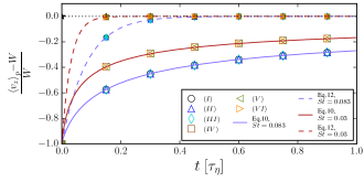
Figure 7: Short-term behavior of the center of mass velocities expressed as $(\left<v_{z}\right>-W)/W$: empty symbols: with memory (Eq. 4), and full symbols: without memory (Eq. 8). Black stars indicate the results for non-inertial particles but only up to $t=0.3\;\tau_{\eta}$ in order to avoid heavy overlap. Continuous (dashed) curve represents the still fluid result with memory (without memory) as expressed by (10) ((12)).

It is interesting to compare the numerical data with the analytic expression presented for the free fall in still fluids in Section III. To this end, we have to rescale equations (10) and (12) according to the units used for the turbulent flow. Since the time unit in still fluid can only be $\tau_{p}$, but in turbulence it is chosen to be the Kolmogorov time $\tau_{\eta}$, and the Stokes number is exactly $\tau_{p}/\tau_{\eta}$ (see Eq.(6)), the dimensionless time $t^{\prime}$ of those equation should be transformed into a $t/St$, where $t$ is the dimensionless time used in all our equations. Simultaneously, $v^{\prime}_{z}$ of the still fluid case should be replaced by $Wv_{z}$ in order to be converted to our units. The different curves in Fig. 7 represent the still fluid results (10) and (12) in these units. Since our six parameter sets are grouped around two Stokes numbers, with which time is scaled, each type of solution appears with two curves. A surprising observation is that all points representing the ensemble averages (symbols) of the turbulent results fall exactly on the still-fluid curves.

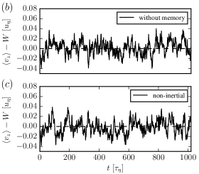
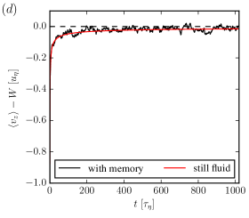
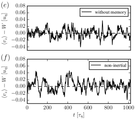
Figure 8: Long-term behavior of the velocity difference $(\left<v_{z}\right>-W)$ for cases I ($a,b,c$) and III ($d,e,f$). The left column ($a,d$) shows the results of the Maxey-Riley equation, the right column those without memory effects. Continuous red lines represent (13) an approximate form of settling in still fluid, and fits nevertheless very well to the turbulent data.

To see the long-term behavior, and check if the relation with the still fluid results hold also on this time scale, we show in Fig. 8 the difference between $W$ and the ensemble averaged vertical velocity up to $1020$ Kolmogorov times. Since the large eddy turnover time $T$ in Table 2 is about $30\tau_{\eta}$, $t=1020$ corresponds to about $34$ turnover times, quite a considerable time span in turbulence. The results of two cases (I and III) are shown in Fig. 8a,d for the Maxey-Riley dynamics with memory, in Fig. 8b,e for the dynamics without memory and in Fig. 8c,f for the non-inertial dynamics. With memory, the ensemble averaged settling velocity is always below $W$, and has not yet reached a steady value by the end of the investigated time interval. This is so even for averages taken over finite time windows of, say, one large eddy turnover time. Such smoothed time series (not shown) are, however, remarkably close to the result valid in still fluid. In order to check if this property is not a consequence of the relatively large settling velocities, we carried out additional simulations with $10$ times smaller $W$-s but the same Stokes numbers as in Table I. The results in turbulent flow are found to correlate with the still fluid settling just as in Figs. 7, 8. In fact, the red lines represent the function:

$$\left<v_{z}\right>(t)=W\left[1-\sqrt{\frac{3St}{\pi t}}\right],$$ (13)

which follows from (11) to be valid asymptotically, and the deviation of $\beta$ from unity can be neglected since all our access densities are rather small. This indicates that the decay towards the asymptotic settling velocity is of power-law type, decaying as one over the square-root of time. Since such functions are scale-free, no characteristic time can be associated with them (in contrast e.g. to exponential decays).

Regarding the right column of panels, note the very small scale on the vertical axes. In all cases the average is zero, meaning that the average settling velocity over the investigated time interval is $W$, as in still water. The graphs of the non-inertial and memoryless dynamics are somewhat different, but they basically represent a random process around zero. Fluctuations in all panels are on the order of $0.05$. These features also hold for the results of the other four cases not shown here.

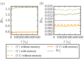
Figure 9: Vertical (left panel) and horizontal (right panel) Reynolds numbers as a function of time for case V (upper curves) and VI (lower curves). The grey horizontal line represents the order of magnitude estimate $Re_{h}^{*}$ of (1).

We also evaluate the slip velocities of the particle ensemble as time series with and without memory and, based on these define an instantaneous vertical and horizontal Reynolds number $Re_{z}(t)$ and $Re_{h}(t)$ in an analogous way as $Re_{z}^{*}$ and $Re_{h}^{*}$ are defined in (1), but this time with the average of the modulus of the instantaneous slip velocity $\left<|\vec{v}(t)-\vec{u}(t)|\right>$. The results obtained for cases V and VI are summarized in Fig. 9. With memory, the vertical Reynolds number converges according to a power law to a long-term limit, which is close to $Re_{z}^{*}=Wa/\eta$, a value the other dynamics reach practically immediately. The order of magnitude of the limiting Reynolds number is unity in all the cases (the values coincide with those given in Table I). The horizontal Reynolds numbers are much smaller than unity. They depend on the access density, and differ a little bit with and without memory. In any case they happen to be close to the estimated value $Re_{h}^{*}=St\;a/\eta$. The difference is changing with W, and we can discover a simple relation

$$\frac{\overline{Re_{hw}}-\overline{Re_{hm}}}{W}=const.$$ (14)

to hold, where index $m$ and $w$ stand for memory and without memory, respectively. The value of the constant is found to be about $0.005$ and $0.0006$ for $St=0.083$ and $St=0.03$, respectively. It reflects that for $W\rightarrow 0$ the particles have smaller and smaller excess densities, and their dynamics approaches that of ideal fluid elements with the zero initial slip velocity condition used in this paper.

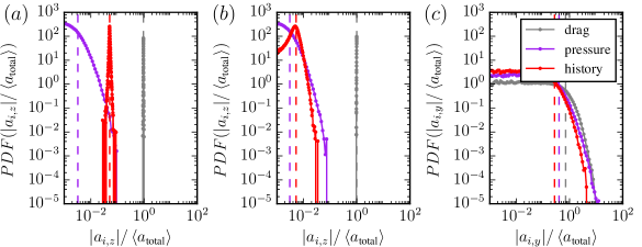
Figure 10: Pdf-s of the accelerations $\vec{a}_{i}$ due to different forces (i=pressure, drag or memory) for case IV (a) $z$ component at time $t=10.5\;\tau_{\eta}$, (b) $z$ component at $t=1020\;\tau_{\eta}$, (c) $y$ component at $t=1020\;\tau_{\eta}$. Vertical dashed lines indicate the ensemble averages. $\left<a_{total}\right>$ denotes the ensemble average of the modulus of the resultant acceleration.

It is worth also considering the distributions (pdf-s) of the different types of accelerations. In Fig. 10 the acceleration due to the drag, pressure and history force are plotted, for case IV, at time instants $t=10.5\;\tau_{\eta}$ and $t=1020\;\tau_{\eta}$ for the vertical, and only for the last instant for the horizontal components. In the vertical, the drag dominates, and has a rather narrow distribution. This is due to the fact that the slip velocity becomes quickly to be of order $W$. On the other hand, the pdf of the acceleration from the pressure term is rather broad and hardly changes with time after $t=10.5\;\tau_{\eta}$. These two pdf-s are found nearly identical with those in the memoryless equations. Only the pdf of the history force (red) changes with time rather dramatically: at $t=10.5\;\tau_{\eta}$ it is sharp an has a much larger average than the pressure contribution. By the end of the observational period, however, the pdf broadens and becomes shifted towards smaller values. Its average remains only slightly larger than that of the pressure. In the horizontal, the distributions are similar, do not change too much in time, the averages are ordered as drag, pressure and history with not very much differences. These pdf-s are rather different from those obtained without gravity in Daitche (2015): all distributions are broad there, the pressure contribution is the largest, those of drag and history are comparable, and the averages are not separated by several orders of magnitudes. The closeness of the averages resembles Fig. 10c.

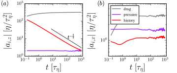
Figure 11: Time dependence of the mean of the different pdf-s shown in the previous figure. Left panel: vertical, right panel: horizontal components. The thin black line in the left panel is of slope $-1/2$ to guide the eye.

To gain insight into the full time dependence, we plot in Fig. 11 the ensemble average of the pdf-s shown above. A striking feature in the vertical components (left panel) is the monotonous decay of the history force. Sooner or later, the average of the history force is likely to become smaller than that of the pressure force. This internal degradation of the history force seems to be specific to the sedimentation dynamics with all the parameters investigated. Horizontally (right panel), however, everything is stationary after $t=10.5$. The relatively small values of the history acceleration explain why no sign of a slow convergence is seen in Fig. 9b. The stationarity of the average pressure acceleration indicates the stationarity of our turbulent flow. Its order of magnitude is indeed $u_{\eta}/\tau_{\eta}=\eta/\tau_{\eta}^{2}$. It is worth noting that the averages of the accelerations themselves without taking the modulus would all be zero with the exception to the vertical drag and vertical history acceleration.

VII Estimating the relevance of the Faxén corrections

The Faxén corrections are corrections to (4) due to the finite size of the particle and to the curvature of the flow. They appear as terms proportional to $a^{2}\Delta\vec{u}$ which are added to the slip velocity in the Stokes drag and in the nominator of the memory integral, as well as to the fluid velocity in the added mass term Maxey and Riley (1983); Gatignol (1983). They appear with a coefficient $1/6$ and $1/10$, respectively. We concentrate here on the correction to the slip velocity and consider the ratio of the average modulus of the correction to that of the slip velocity

$$C_{j}=\frac{a^{2}}{6}\frac{\left<|\Delta\vec{u}_{j}|\right>}{\left<|\vec{v}_{j}-\vec{u}_{j}|\right>},$$ (15)

where index $j$ stands for the Cartesian components $x,y$ or $z$ in this correction factor. Because of the anisotropy due to gravity, it is worth treating the horizontal and vertical components separately. Their difference becomes clear from a simple estimation. Since the characteristic length and velocity scale of the turbulent flow are $\eta$ and $u_{\eta}$, respectively, the Laplacian in any component can be estimated as $u_{\eta}/\eta^{2}$. The slip velocity in the vertical is approximately $Wu_{\eta}$, while that in the horizontal is $Stu_{\eta}$, as used in (3). We thus find the estimates for the vertical and horizontal correction factors

$$C^{*}_{z}=\frac{1}{6}\left(\frac{a}{\eta}\right)^{2}\frac{1}{W},\;\;\;C^{*}_{h}=\frac{1}{6}\left(\frac{a}{\eta}\right)^{2}\frac{1}{St}.$$

Since $W$ is larger than unity in our cases, but $St<1$ (see Table I.), the relative importance of the Faxén corrections is expected to be much smaller in vertical than in horizontal direction. For our largest particles $a/\eta=1/2$, and $St=0.083$, thus the estimate $C^{*}_{h}$ amounts to a value $0.5$.

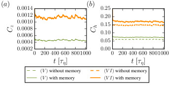
Figure 12: Time dependent correction factor $C_{z}$ (a) and $C_{x}$ (b) for case (V) and (VI) with memory and without memory.

We numerically determine the correction factors $C_{j}$ as functions of time. The results in the presence of memory are shown in Fig. 12 for $C_{z}$ and $C_{x}$ for cases (V) and (VI) with and without memory. The vertical corrections (Fig. 12a) appear to be at most $0.1$ % consistently, with hardly any difference with and without memory. For smaller excess density (case (VI)) the correction is larger. The measured values are about a factor 5 smaller than the estimates $C^{*}_{z}$. In the horizontal, the corrections factor reaches nearly $20$ %, but is about a factor 3 smaller than what the estimate $C^{*}_{h}$ predicts. There is a measurable difference in the correction with memory and without, and the former one is consistently larger by about $10$ %. The effect for lighter particles is here stronger again. A comparison with Fig. 9 reveals that the tendencies in the Reynolds numbers and in the correction factors are roughly the opposites.

We thus find that in the vertical Faxén corrections can safely be neglected. In the horizontal, the Faxén corrections might be on the same order, but yet smaller, as the slip velocity. We found, however, the horizontal slip velocity to be small compared to unity (see Fig. 9b). Modifying this difference by a factor smaller than unity does not change the basic observation of the paper that the horizontal Reynolds number is small, i.e. that the particles follow in the horizontal direction the fluid motion very closely.

VIII Conclusions

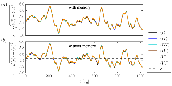
Figure 13: Time dependence of the vertical velocity variance of the ensembles, of the different cases marked with different colors. (a): with memory, (b) without memory. The horizontal dashed lines mark the temporal average $\overline{\sigma}$ of these quantities averaged over all cases. These values happen to be identical for the two dynamics, and close to the velocity variance of the turbulent flow.

Inspired by the sedimentation of marine snow particles in the ocean, we have studied the impact of the history force on the sedimentation of almost neutrally buoyant spherical particles in a three-dimensional turbulent flow. Our study is based on the Maxey-Riley equation and we compared our results with the dynamics of particles when neglecting the history force, as well as, with non-inertial particles. We have analyzed 6 parameter sets for marine snow particles corresponding to typical situations in estuaries and the open ocean. We have shown that the history force, which introduces a memory, cannot be neglected.While it leads to large deviations of the trajectories of individual particles from the ones without memory or of non-inertial particles, the differences in the horizontal dynamics and spatial extensions of ensemble of particles are not that large. The most striking effect concerns the vertical dynamics: when the history force is taken into account, the vertical velocity of the center of mass of the cloud approaches very slowly a constant settling velocity, according to a one-over-square-root of time law.

Furthermore, our results indicate that for all three approaches the settling of small particles, possessing a density not much larger than the one of the fluid, is surprisingly well described in turbulence by the settling in a still fluid. The history force leads to a much slower convergence to the settling velocity, and the limit has not even be reached after more than 1000 Kolmogorov times. This convergence is of power-law type and we demonstrated a simple, general expression in the form of (13) to hold.

By contrast, the "ad hoc" dynamics obtained by neglecting the memory converge to the settling velocity even within one Kolmogorov time unit. The turbulent motion of the fluid manifests itself in both cases only in fluctuations around the settling velocity, which are determined by the properties of the flow. We illustrate this finding by showing in Fig. 13 the time dependence of the vertical velocity variance for all the cases in a single panel, marked with different colors. On the scale of $1000$ Kolmogorov units they hardly differ, and the overall shape is very similar both in the Maxey-Riley equation with memory (Fig. 13a), and for inertial particles without memory (Fig. 13b). One hardly sees any difference with naked eye, and this also holds for the result obtained with non-inertial particles (not shown). Given that the velocity variance is 5.4 Kolmogorov units in the turbulent flow (see Table II.), we conclude that it is mainly the flow that determines the particle dynamics, as the particles are very close in their densities to that of the fluid. The variance due to particle properties and advection dynamics only appears in the width of the plotted curves. This width is about 1% on this scale, which is in line with the observed velocity fluctuations being less than 0.05 in Fig. 8. Changes in the variance as well as in the vertical velocity difference happen on a timescale which is comparable to the large-eddy turnover time of about 30 Kolmogorov times.

There has been an extensive study of settling of inertial particles in turbulent fluids by Wang & Maxey Wang and Maxey (1993) although without memory effects. Though their analysis differs from ours in several aspects, we find it interesting to compare our results with theirs. Wang & Maxey Wang and Maxey (1993) have considered only the Stokes drag and the gravity as the forces acting on their particles, i.e. their study applies to very heavy particles ($\rho_{p}>>\rho_{f}$) instead of the light particles on which we focus. One of their main achievements consists in the finding that turbulent motion leads to an additional acceleration of the particles resulting in an enhanced settling velocity. Their explanation is based on the strongly inhomogeneous distribution of their heavy particles due to the formation of preferential concentrations in the flow. Due to inertia the heavy particles are expelled from the vortices in the flow and whenever they encounter a vortex during settling they will be accelerated in the direction of its rotation which moves it into the direction of the downwards motion of the fluid. In our case of very light particles we do not observe preferential concentration, the particles are almost homogeneously distributed. These light particles, experiencing additionally the pressure and the history force, exhibit a dynamics which is closer to that of non-inertial particles, for which such a net effect on the average settling velocity can not be expected. The latter conjecture has already been formulated by Wang & Maxey Wang and Maxey (1993); Maxey (1987) and our study seems to confirm that. To be able to observe preferential concentration for such light particles we would have to go beyond the scope of the Maxey-Riley equation.

Introducing gravity into the dynamics of inertial particles reveals that the settling velocity appears as another important parameter besides the Stokes number. One could argue that the effect of the turbulent fluid flow on the settling of particles could be more pronounced when the settling velocity is larger than the one for our light particles. However, looking at the particle Reynolds numbers it turned out that one can distinguish between a vertical particle Reynolds number $Re_{z}$ and a horizontal one $Re_{h}$. Because the horizontal one scales with the Stokes number which is very small for our cases, the particle Reynolds number is largely determined by the vertical one which scales with the settling velocity. These estimates for the two components of the particle Reynolds number reveal the difficulty in studying particles with larger settling velocities due to larger densities: the vertical particle Reynolds number would increase in such a way, that the Maxey-Riley equation would not be valid anymore. This equation is known to be valid Daitche (2015) under the assumption that the particle Reynolds number is smaller or approximately unity, which would be violated for heavy particles.

We find striking differences between the horizontal and the vertical components of the forces acting on the particle. While the horizontal components of the drag, the pressure and the history force are almost constant after some transient time, this applies only to the vertical components of drag and pressure. The vertical component of the history force, however, becomes smaller and smaller as time goes by. This can be interpreted as an indicator for that this force does not have an essential influence on the asymptotic settling velocity.

Let us add a remark on cases when marine aggregates of different sizes and of different excess densities are considered simultaneously, as a superensemble, with some size and density distribution. To understand their typical settling dynamics, it is worth rewriting the leading term in (11) in dimensional units. After averaging, this leads to

$$\bigg{\langle}\frac{W_{\text{settling}}-\left<v_{z}\right>(t)}{W_{\text{settling}}}\bigg{\rangle}_{s}\approx\frac{\left<a\right>_{s}}{\sqrt{\pi\nu t}}.$$

In the turbulent context, $\left<v_{z}\right>$ means the average vertical velocity of the particle cloud of a given size and density, and $\left<\right>_{s}$ stands for the average taken over the superensemble of different marine aggregates. Since the right hand side is independent of the density  (and also of the fluid properties), the average of the relative deviation from the asymptotic settling velocity will be proportional to the average size in the superensemble. The larger this size, the slower the convergence. For an average size of $1$ mm, and with the viscosity of water, $\nu=10^{-6}$ in SI units, for example, the deviation remains more than one percent, for $t<10^{4}/3$ s, i.e. for practically one hour. The convergence to a uniform settling velocity is thus expected to be rather slow also in a superensemble, due to the history force.

Finally we would like to briefly turn to the settling of plankton. These can be considered as particles of more or less the same excess density as marine snow, but a factor of 10 smaller in size, with a typical radius of 10 micrometers. The effect of the history on the settling of plankton was numerically studied by Olivieri in his thesis Olivieri (2013). He chose two parameter sets, both with very small $St$ and $W$. The weak effect of gravity leads to dynamics where the action of all forces is almost isotropic, and the difference between the horizontal and the vertical directions is small. Although he observes some deviations from $W$ for the vertical velocity, he attributes them to statistical fluctuations and concludes that these small microorganisms will be carried by the flow as non-inertial tracers. This is in harmony with our findings since a change to a=10 micrometers (corresponding to a typical plankton cell) a factor 30-50 smaller than our aggregates, would make even the one-over-square-root type decay to appear very fast.

IX Acknowledgment

T.T. acknowledges the support of OTKA grant NK100296 and of the Alexander von Humboldt Foundation. We are grateful to George Jackson for illuminating discussions. U.F. would like to thank T. Tél and his group for hospitality during the stay at Eötvös University Budapest and the Hungarian Academy of Sciences for financial support.

Appendix A

In order to test how an initially strongly localized ensemble behaves, we carried out a single extra simulation with $N_{p}=5\cdot 10^{4}$ particles uniformly distributed at time $t=0$ in a box of size $L=1\cdot\eta$ centered at the origin, with zero initial slip velocities. Since the differences among the three types of dynamics are minor for the ensemble variances, here we chose non-inertial and inertial particles without memory only, since they require lower computational demand. The simulation is carried out up to 300 $\tau_{\eta}$. The variances are shown in Fig. 14. In contrast to Fig. 6, here a clear intermediate time scaling with $t^{3}$ can be found, i.e., Richardson’s scaling becomes observable. A difference between the horizontal and the vertical dynamics is that in the latter (panel b) ballistic behaviour is not observable in the data.

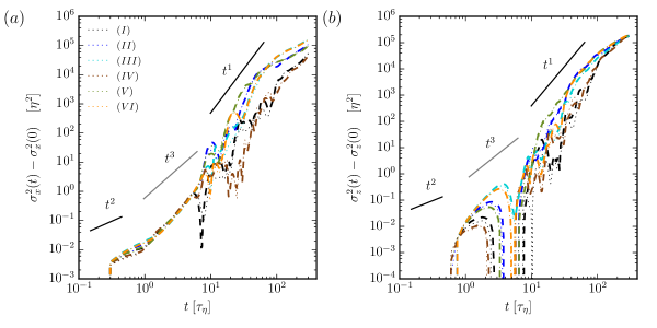
Figure 14: Time-dependence of the variances in the horizontal (x, (a)) and vertical (z, (b)) directions in the different cases (coloring and line types as in the previous figures) on log-log scales. The ensemble is initiated in a box of $L=1\;\eta$. For clarity, the initial variance ($\sigma_{x}(0)=1/\sqrt{12}=0.287\;\eta$) is subtracted. Straight lines with slopes 1,2 and 3 are overlaid to lead the eye.

It is worth determining the dimensionless crossover time $t_{0}/\tau_{\eta}$ for this case, too. Along the lines applied in Section V, we find

$$\frac{t_{0}}{\tau_{\eta}}=(3\sigma^{2}_{x}(0))^{1/3}=(3/12)^{1/3}=0.630.$$ (16)

This corresponds precisely to the time where a crossover from the quadratic to the cubic, Richardson scaling takes place. Note that the second crossover from the Richardson to a diffusive behavior occurs at about 30 $\tau_{\eta}$, i.e. at the eddy turnover time $T$. The lack of the Richardson regime in Fig. 6 is due to the fact that the turnover time $t_{0}$ is larger than $T$, and hence there is no "space" for the cubic behavior.

References

- Tanga and Provenzale (1994) P. Tanga and A. Provenzale, Physica D: Nonlinear Phenomena 76, 202 (1994).
- Belmonte et al. (2001) A. Belmonte, J. Jacobsen, and A. Jayaraman, All HMC Faculty Publications and Research (2001).
- Daitche and Tél (2011) A. Daitche and T. Tél, Physical Review Letters 107, 244501 (2011), 00007.
- Guseva et al. (2013) K. Guseva, U. Feudel, and T. Tél, Physical Review E 88, 042909 (2013).
- Daitche and Tél (2014) A. Daitche and T. Tél, New Journal of Physics 16, 073008 (2014).
- Farazmand and Haller (2015) M. Farazmand and G. Haller, Nonlinear Analysis: Real World Applications 22, 98 (2015).
- Mordant and Pinton (2000) N. Mordant and J.-F. Pinton, The European Physical Journal B 18, 343 (2000).
- Candelier et al. (2004) F. Candelier, J. R. Angilella, and M. Souhar, Physics of Fluids 16, 1765 (2004).
- Vojir and Michaelides (1994) D. Vojir and E. Michaelides, International Journal of Multiphase Flow 20, 547 (1994), 00077.
- Langlois et al. (2015) G. P. Langlois, M. Farazmand, and G. Haller, Journal of Nonlinear Science , 1 (2015).
- Daitche (2015) A. Daitche, Journal of Fluid Mechanics 782, 567 (2015).
- Maxey and Riley (1983) M. R. Maxey and J. J. Riley, Physics of Fluids 26, 883 (1983).
- Gatignol (1983) R. Gatignol, J. Mec. Theor. Appl 1, 143 (1983).
- Auton et al. (1988) T. R. Auton, J. C. R. Hunt, and M. Prud’Homme, Journal of Fluid Mechanics 197, 241 (1988), 00348.
- Basset (1888) A. B. Basset, A Treatise on Hydrodynamics (Deighton, Bell and Co., 1888).
- van Hinsberg et al. (2011) M. van Hinsberg, J. ten Thije Boonkkamp, and H. Clercx, Journal of Computational Physics 230, 1465 (2011), 00028.
- Daitche (2013) A. Daitche, Journal of Computational Physics 254, 93 (2013).
- Toegel et al. (2006) R. Toegel, S. Luther, and D. Lohse, Physical Review Letters 96, 114301 (2006).
- Garbin et al. (2009) V. Garbin, B. Dollet, M. Overvelde, D. Cojoc, E. Di Fabrizio, L. van Wijngaarden, A. Prosperetti, N. de Jong, D. Lohse, and M. Versluis, Physics of Fluids 21, 092003 (2009), 00015.
- Bergougnoux et al. (2014) L. Bergougnoux, G. Bouchet, D. Lopez, and E. Guazzelli, Physics of Fluids (1994-present) 26, 093302 (2014).
- Aartrijk and Clercx (2010) M. v. Aartrijk and H. J. H. Clercx, Physics of Fluids (1994-present) 22, 013301 (2010).
- Olivieri (2013) S. Olivieri, Analysis of the Forces Acting on Particles in Homogeneous Isotroic Turbulence, Ph.D. thesis, Università degli Studi di Genova, Genova (2013).
- Mann and Lazier (2005) K. Mann and J. Lazier, Dynamics of Marine Ecosystems: Biological-Physical Interactions in the Oceans, 3rd ed. (Wiley-Blackwell, 2005).
- De La Rocha and Passow (2007) C. L. De La Rocha and U. Passow, Deep Sea Research Part II: Topical Studies in Oceanography 54, 639 (2007), 00086.
- Riley et al. (2012) J. S. Riley, R. Sanders, C. Marsay, F. a. C. Le Moigne, E. P. Achterberg, and A. J. Poulton, Global Biogeochemical Cycles 26 (2012), 00009.
- Stone (2010) R. Stone, Science 328, 1476 (2010).
- Passow and Carlson (2012) U. Passow and C. A. Carlson, Marine Ecology Progress Series 470, 249 (2012), 00006.
- McDonnell and Buesseler (2010) A. M. P. McDonnell and K. O. Buesseler, Limnology and Oceanography 55, 2085 (2010).
- Petrik et al. (2013) C. M. Petrik, G. A. Jackson, and D. M. Checkley Jr., Deep Sea Research Part I: Oceanographic Research Papers 74, 64 (2013).
- Gargett (1989) A. E. Gargett, Annual Review of Fluid Mechanics 21, 419 (1989).
- Murray (1970) S. P. Murray, Journal of Geophysical Research 75, 1647 (1970).
- Tooby et al. (1977) P. F. Tooby, G. L. Wick, and J. D. Isaacs, Journal of Geophysical Research 82, 2096 (1977).
- Alldredge and Gotschalk (1988) A. L. Alldredge and C. Gotschalk, Limnology and Oceanography 33, 339 (1988).
- Shanks (2002) A. L. Shanks, Continental Shelf Research 22, 2045 (2002).
- Ruiz et al. (2004) J. Ruiz, D. Macías, and F. Peters, Proceedings of the National Academy of Sciences of the United States of America 101, 17720 (2004).
- Note (1) The effective density is not easy to determine directly, but is often inferred from measured settling velocities based on the assumption of the validity of the Stokes law or of a modification thereof.
- Kranenburg (1994) C. Kranenburg, Estuarine, Coastal and Shelf Science 39, 451 (1994).
- Winterwerp (1998) J. C. Winterwerp, Journal of Hydraulic Research 36, 309 (1998).
- Logan and Wilkinson (1990) B. E. Logan and D. B. Wilkinson, Limnology and Oceanography 35, 130 (1990).
- Khelifa and Hill (2006) A. Khelifa and P. S. Hill, Journal of Hydraulic Research 44, 390 (2006).
- Jackson et al. (2005) G. A. Jackson, A. M. Waite, and P. W. Boyd, Geophysical Research Letters 32, L13607 (2005).
- Zahnow et al. (2011) J. C. Zahnow, J. Maerz, and U. Feudel, Physica D: Nonlinear Phenomena 240, 882 (2011), 00004.
- McCave (1984) I. N. McCave, Deep Sea Research Part A. Oceanographic Research Papers 31, 329 (1984).
- Tambo and Watanabe (1979) N. Tambo and Y. Watanabe, Water Research 13, 409 (1979).
- Simon et al. (2002) M. Simon, H. P. Grossart, B. Schweitzer, and H. Ploug, Aquatic microbial ecology 28, 175 (2002).
- Soulsby et al. (2013) R. L. Soulsby, A. J. Manning, J. Spearman, and R. J. S. Whitehouse, Marine Geology 339, 1 (2013).
- Winterwerp (2011) J. C. Winterwerp, in Treatise on Estuarine and Coastal Science, edited by E. Wolanski and D. McLusky (Academic Press, Waltham, 2011) pp. 311–360.
- Oakey and Elliott (1982) N. S. Oakey and J. A. Elliott, Journal of Physical Oceanography 12, 171 (1982).
- Kirboe and Saiz (1995) T. Kirboe and E. Saiz, Marine Ecology Progress Series 122, 135 (1995).
- Bartholomä et al. (2009) A. Bartholomä, A. Kubicki, T. H. Badewien, and B. W. Flemming, Ocean Dynamics 59, 213 (2009), 00029.
- Note (2) For small excess densities , characteristic to our cases, , as follows from Eq.( 5) for small .
- Pope (2000) S. B. Pope, Turbulent Flows, 1st ed. (Cambridge University Press, 2000).
- Canuto et al. (1987) C. Canuto, M. Y. Hussaini, A. Quarteroni, and T. A. Zang, Spectral Methods in Fluid Dynamics (Springer Berlin Heidelberg, Berlin, Heidelberg, 1987).
- Hou and Li (2007) T. Y. Hou and R. Li, Journal of Computational Physics 226, 379 (2007).
- Shu and Osher (1988) C.-W. Shu and S. Osher, Journal of Computational Physics 77, 439 (1988).
- Note (3) Given the same initial condition on the same computer (i.e. floating-point architecture) with a fixed time step, would not lead to a separation of two runs even in chaos with any chosen equation of motion. Note that the deviations generated by our three different dynamics can be additionally amplified by the chaotic nature of the particle dynamics. Here, were are unable to separate out this amplification.
- Note (4) The limit of can only be considered for mathematical convenience. In the case of finite size particles it is important to remain in the dilute limit, in order to avoid hydrodynamic interactions.
- Batchelor (1950) G. K. Batchelor, Quarterly Journal of the Royal Meteorological Society 76, 133 (1950).
- Wang and Maxey (1993) L.-P. Wang and M. R. Maxey, Journal of Fluid Mechanics 256, 27 (1993).
- Maxey (1987) M. R. Maxey, Journal of Fluid Mechanics 174, 441 (1987).
- Note (5) The excess density is important, of course, for , see also (7), but not for the ratio investigated here.