About 30 Years of Integrable Chiral Potts Model, Quantum Groups at Roots of Unity and Cyclic Hypergeometric Functions

Abstract.

In this paper we discuss the integrable chiral Potts model, as it clearly relates to how we got befriended with Vaughan Jones, whose birthday we celebrated at the Qinhuangdao meeting. Remarkably we can also celebrate the birthday of the model, as it has been introduced about 30 years ago as the first solution of the star-triangle equations parametrized in terms of higher genus functions. After introducing the most general checkerboard Yang–Baxter equation, we specialize to the star-triangle equation, also discussing its relation with knot theory. Then we show how the integrable chiral Potts model leads to special identities for basic hypergeometric series in the $q$ a root-of-unity limit. Many of the well-known summation formulae for basic hypergeometric series do not work in this case. However, if we require the summand to be periodic, then there are many summable series. For example, the integrability condition, namely, the star-triangle equation, is a summation formula for a well-balanced ${}_{4}\Phi_{3}$ series. We finish with a few remarks about the relation with quantum groups at roots of unity.

1. How we got to know Vaughan Jones

In 1988 one of us found a preprint by Vaughan Jones, “On a Certain Value of the Kauffman Polynomial” [1]. We immediately saw that the metaplectic representation for $p=5$ therein had to be related to our chiral Potts model work [2, 3] and it soon became clear that it was even related to the 5-state Fateev–Zamolodchikov model [4].

After reporting this to Vaughan we received an invitation to the Workshop on Integrable Systems in Statistical Mechanics, Quantum Field Theory, and Knot Theory, at MSRI, UC Berkeley, January 1989. There we both had detailed further discussions on the relationships between knot theory and integrable models of statistical mechanics and some of that got incorporated in the paper “On Knot Invariants Related to Some Statistical Mechanical Models” [5].

One evening during the workshop, Vaughan invited us both to his apartment, but Helen could not go as our baby was not well. At one point Vaughan came up with five copies of Händel’s Messiah for five of us present. He then assigned the four voice parts, “Jacques, do you want to sing tenor or bass?” and Anthony Wasserman got the piano accompaniment. Thus we performed the entire piece from cover to cover. It was a deeply spiritual experience with the entire text taken from the King James Version of the Bible.

We have met Vaughan later at several other meetings and have played several games of snooker together. Once during a conference honoring Baxter in Canberra we had a bus trip to Tidbinbilla. Vaughan said, “Helen, you have to sit somewhere else; I have to sit next to Jacques.” and we sang several parts of the Messiah together. Even during the Great Wall expedition of the Qinhuangdao conference we sang ‘Comfort ye’ and ‘Every valley’ in the bus after Helen fell asleep and her earplug came loose from her iPad.

2. Yang–Baxter integrable statistical mechanics models

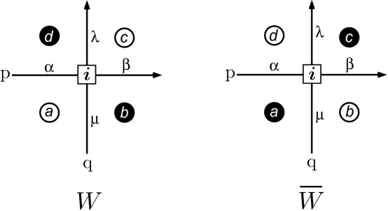
Figure 1. The Boltzmann weights $W{}^{(i)}{}^{\lambda\beta}_{\alpha\mu}|{}^{dc}_{ab}(p,q)$ and $\overline{W}{}^{(i)}{}^{\lambda\beta}_{\alpha\mu}|{}^{dc}_{ab}(p,q)$

associated with the crossing of oriented rapidity lines with rapidities p and q. Spin variables live on line pieces, faces and vertices. Faces are colored alternatingly black and white in a checkerboard pattern.

The Yang–Baxter equation [6, 7] is a generalization of Artin’s braid equation in knot theory with spectral variables called rapidities $\mathrm{p},\mathrm{q},\cdots$, living on oriented lines, see figure 1. To each crossing of the rapidity lines one assigns Boltzmann weights $W{}^{(i)}{}^{\lambda\beta}_{\alpha\mu}|{}^{dc}_{ab}(p,q)$ or $\overline{W}{}^{(i)}{}^{\lambda\beta}_{\alpha\mu}|{}^{dc}_{ab}(p,q)$ depending on a black-white checkerboard coloring assigned to the faces. Most generally, one can have spin variables on all faces, vertices and line pieces, while each spin variable can be chosen independently from a finite or infinite set.

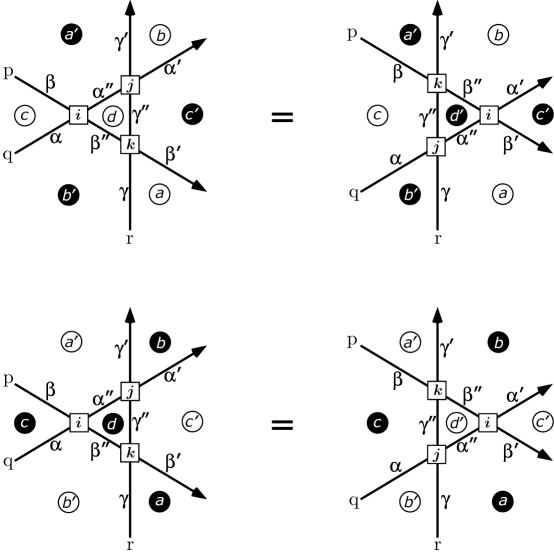
Figure 2. Pictorial representation of the checkerboard Yang–Baxter equations. State sums over spins on the vertices and on internal faces and line pieces are assumed.

One can sum over the spin $i$ at the vertex, obtaining the IRF-vertex model with new Boltzmann weights $\sum_{i}W{}^{(i)}{}^{\lambda\beta}_{\alpha\mu}|{}^{dc}_{ab}(p,q)\equiv W{}^{\lambda\beta}_{\alpha\mu}|{}^{dc}_{ab}(p,q)$, $\sum_{i}\overline{W}{}^{(i)}{}^{\lambda\beta}_{\alpha\mu}|{}^{dc}_{ab}(p,q)\equiv\overline{W}{}^{\lambda\beta}_{\alpha\mu}|{}^{dc}_{ab}(p,q)$. Such a reduction can always be applied and has been useful in certain spin models, see e.g. [8, 9, 10].

Assuming that there are no spins at the intersections of rapidity lines, one can define several special cases [7]. First, if the spins on the line pieces ($\alpha,\beta,\cdots$) only take a single value, one can omit them, arriving at the checkerboard Interaction-Round-a-Face (IRF) model with weights $W{}^{dc}_{ab}(p,q)$, $\overline{W}{}^{dc}_{ab}(p,q)$. Second, assuming all spins on the faces have a single value (and thus can be omitted) one receives the checkerboard vertex model with weights $W{}^{\lambda\beta}_{\alpha\mu}(p,q)$, $\overline{W}{}^{\lambda\beta}_{\alpha\mu}(p,q)$. Forgetting about the coloring of the faces one gets the usual vertex model with $W{}^{\lambda\beta}_{\alpha\mu}(p,q)=\overline{W}{}^{\lambda\beta}_{\alpha\mu}(p,q)$. Finally, if one only leaves spins on the black (or white) faces, one ends up with a spin model.

The most general Yang–Baxter equation is depicted in figure 2 and can be expressed more complicatedly in formula as

(1) $$\sum_{i}\sum_{j}\sum_{k}\sum_{\alpha^{\prime\prime}}\sum_{\beta^{\prime\prime}}\sum_{\gamma^{\prime\prime}}\sum_{d}W{}^{(i)}{}^{\alpha^{\prime\prime}\!\beta^{\prime\prime}}_{\beta\,\,\alpha}\!|{}^{a^{\prime}d}_{c\,b^{\prime}}(p,q)$$

$$\hskip 60.00009pt\times\,W{}^{(j)}{}^{\gamma^{\prime}\,\alpha^{\prime}}_{\alpha^{\prime\prime}\gamma^{\prime\prime}}\!|{}^{a^{\prime}b}_{d\,c^{\prime}}(q,r)\,\overline{W}{}^{k)}{}^{\gamma^{\prime\prime}\beta^{\prime}}_{\beta^{\prime\prime}\gamma}\!|{}^{d\,c^{\prime}}_{b^{\prime}a}(p,r)$$

$$\quad=R(p,q,r)\,\sum_{i}\sum_{j}\sum_{k}\sum_{\alpha^{\prime\prime}}\sum_{\beta^{\prime\prime}}\sum_{\gamma^{\prime\prime}}\sum_{d^{\prime}}\overline{W}{}^{(i)}{}^{\alpha^{\prime}\,\beta^{\prime}}_{\beta^{\prime\prime}\alpha^{\prime\prime}}\!|{}^{b\,c^{\prime}}_{d^{\prime}a}(p,q)$$

$$\hskip 60.00009pt\times\,\overline{W}{}^{(j)}{}^{\gamma^{\prime\prime}\!\alpha^{\prime\prime}}_{\alpha\,\,\gamma}\!|{}^{c\,d^{\prime}}_{b^{\prime}a}(q,r)\,W{}^{(k)}{}^{\gamma^{\prime}\beta^{\prime\prime}}_{\beta\,\gamma^{\prime\prime}}\!|{}^{a^{\prime}b}_{c\,d^{\prime}}(p,r),$$

(2)

(3) $$\overline{R}(p,q,r)\,\sum_{i}\sum_{j}\sum_{k}\sum_{\alpha^{\prime\prime}}\sum_{\beta^{\prime\prime}}\sum_{\gamma^{\prime\prime}}\sum_{d}\overline{W}{}^{(i)}{}^{\alpha^{\prime\prime}\!\beta^{\prime\prime}}_{\beta\,\,\alpha}\!|{}^{a^{\prime}d}_{c\,b^{\prime}}(p,q)$$

$$\hskip 60.00009pt\times\,\overline{W}{}^{(j)}{}^{\gamma^{\prime}\,\alpha^{\prime}}_{\alpha^{\prime\prime}\gamma^{\prime\prime}}\!|{}^{a^{\prime}b}_{d\,c^{\prime}}(q,r)\,W{}^{(k)}{}^{\gamma^{\prime\prime}\beta^{\prime}}_{\beta^{\prime\prime}\gamma}\!|^{d\,c^{\prime}}_{b^{\prime}a}(p,r)$$

(4) $$\quad=\sum_{i}\sum_{j}\sum_{k}\sum_{\alpha^{\prime\prime}}\sum_{\beta^{\prime\prime}}\sum_{\gamma^{\prime\prime}}\sum_{d^{\prime}}W{}^{(i)}{}^{\alpha^{\prime}\,\beta^{\prime}}_{\beta^{\prime\prime}\alpha^{\prime\prime}}\!|{}^{b\,c^{\prime}}_{d^{\prime}a}(p,q)$$

$$\hskip 60.00009pt\times\,W{}^{(j)}{}^{\gamma^{\prime\prime}\!\alpha^{\prime\prime}}_{\alpha\,\,\gamma}\!|{}^{c\,d^{\prime}}_{b^{\prime}a}(q,r)\,\overline{W}{}^{(k)}{}^{\gamma^{\prime}\beta^{\prime\prime}}_{\beta\,\gamma^{\prime\prime}}\!|{}^{a^{\prime}b}_{c\,d^{\prime}}(p,r).$$

One can read more about this and the various formal equivalences and specializations in [7, 11]. As said before, the sums over $i$, $j$ and $k$ can be taken introducing new sum weights and one can specialize further to get the various special versions of the Yang–Baxter equation in the literature.

Finally, in some examples that we have studied the scalar factors $R(p,q,r)$ and $\overline{R}(p,q,r)$ can be factorized and absorbed into the $W$’s and $\overline{W}$’s by properly redefining these. Also (1) and (3) are the same equation in the integrable chiral Potts model, for example.

3. Integrable chiral Potts model

Let us from now on specialize to the integrable chiral Potts model [2, 3]. Potts means here that there is a translation invariance in the spin variables, meaning that each weight is of the form $W_{a}^{b}(p,q)\equiv W_{pq}(a-b)$ or $\overline{W}_{a}^{b}(p,q)\equiv\overline{W}_{pq}(a-b)$, depending only on the difference of two spin variables $a$ and $b$ modulo an integer $N$ and integrability implies the existence of the two rapidities $p$ and $q$. The chiral property means that there is no reflection invariance, i.e. $W_{pq}(a-b)\neq W_{pq}(b-a)$, $\overline{W}_{pq}(a-b)\neq\overline{W}_{pq}(b-a)$ in general.

The two weights are depicted in figure 3 and have the form

Figure 3. The chiral Potts model weights.

(5) $$\displaystyle W_{pq}(n)=W_{pq}(0)\prod^{n}_{j=1}\biggl{(}\frac{\mu_{p}}{\mu_{q}}\cdot\frac{y_{q}-x_{p}\omega^{j}}{y_{p}-x_{q}\omega^{j}}\biggr{)},$$

$$\displaystyle{\overline{W}}_{pq}(n)={\overline{W}}_{pq}(0)\prod^{n}_{j=1}\biggl{(}\mu_{p}\mu_{q}\cdot\frac{\omega x_{p}-x_{q}\omega^{j}}{y_{q}-y_{p}\omega^{j}}\biggr{)},$$

where $n=a-b$, $\omega=\exp(2\pi\sqrt{-1}/N)$ is an $N$th root of unity, and the two rapidities $p=(x_{p},y_{p},\mu_{p})$ and $q=(x_{q},y_{q},\mu_{q})$ lie on the high-genus curve

(6) $$x_{p}^{N}+y_{p}^{N}=k(1+x_{p}^{N}y_{p}^{N}),\qquad\displaystyle\mu_{p}^{N}=\frac{k^{\prime}}{1-k\,x_{p}^{N}}=\frac{1-k\,y_{p}^{N}}{k^{\prime}},$$

with some $k$ and $k^{\prime}$ satisfying $k^{2}+k^{\prime 2}=1$. Here we shall choose the normalization $W_{pq}(0)=\overline{W}_{pq}(0)=1$.

These weights satisfy the Reflection Relation

(7) $$W_{pp}(a-b)=1,\quad W_{pq}(a-b)W_{qp}(a-b)=1,$$

and Inversion Relation

(8) $$\sum_{b=0}^{N-1}\overline{W}_{pq}(a-b)\overline{W}_{qp}(b-c)=r_{pq}\delta_{a,c}.$$

These relations correspond to Reidemeister moves I and II of knot theory. Indeed,

Figure 4. Identities related to Reidemeister moves I and II. On the left there is a summation over the internal spin $a$, so that $c^{\prime}=c$. On the right there is a summation over internal spin $d$, so that $a^{\prime}=a$.

(9) $$W_{pp}(n)=\Big{(}\frac{\mu_{p}}{\mu_{p}}\Big{)}^{\!\!n}\prod_{j=1}^{n}\frac{y_{p}-x_{p}\omega^{j}}{y_{p}-x_{p}\omega^{j}},\quad\hbox{or}\quad{W_{pp}(a-b)=1},$$

(10) $$\overline{W}_{pp}(n)=\big{(}{\mu_{p}\mu_{p}}\big{)}^{\!n}\!\prod_{j=1}^{n}\frac{\omega x_{p}\!-\!x_{p}\omega^{j}}{y_{p}\!-\!y_{p}\omega^{j}},\quad\hbox{or}\quad{\overline{W}_{pp}(a-b)=\delta_{a,b}}.$$

corresponds to Reidemeister move I and

(11) $$W_{pq}(n)\!=\!\Big{(}\frac{\mu_{p}}{\mu_{q}}\Big{)}^{\!\!n}\prod_{j=1}^{n}\frac{y_{q}-x_{p}\omega^{j}}{y_{p}-x_{q}\omega^{j}}=W^{-1}_{qp}(n),$$

$$\hbox{or}\quad{W_{pq}(b-c)W_{qp}(b-c)=1},$$

(12) $${\sum_{d=0}^{N-1}\overline{W}_{pq}(a-d)\overline{W}_{qp}(d-a^{\prime})=r_{pq}\delta_{a,a^{\prime}}},$$

with some factor $r_{pq}$, corresponds to Reidemeister move II. These are depicted in figure 4.

Finally there is the Star-Triangle Relation (Yang–Baxter relation for the chiral Potts model), see also figure 5,

(13) $$\sum^{N}_{d=1}\,{\overline{W}}_{pr}(a-d)\,W_{pq}(d-c)\,{\overline{W}}_{rq}(d-b)$$

$$\qquad\qquad=R_{pqr}\,\overline{W}_{pq}(a-b)\,{W}_{pr}(b-c)\,W_{rq}(a-c),$$

corresponding to Reidemeister move III.

Figure 5. Spin-model Yang–Baxter (or Star-Triangle) Equation generalizing Reidemeister move III.

As is well known, repeated application of the Star-Triangle Relation, see figure 6, implies that transfer matrices commute. Defining

$=$

Figure 6. Commuting Transfer Matrices: Shown here is the result of repeated application of the Star-Triangle Equation. Applying an additional $qr$ weight to the right before closing the $q$ and $r$ rapidity lines, we can apply the inversion relation and prove that the transfer matrices commute.

(14) $$({T}_{q})_{\sigma,\sigma^{\prime}}=\prod_{j=1}^{L}\,W_{pq}(\sigma_{j},\sigma^{\prime}_{j}){\overline{W}}_{pq}(\sigma_{j+1},\sigma^{\prime}_{j}),$$

$$(\hat{T}_{r})_{\sigma,\sigma^{\prime}}=\prod_{j=1}^{L}\,\overline{W}_{pr}(\sigma_{j},\sigma^{\prime}_{j}){W}_{pr}(\sigma_{j},\sigma^{\prime}_{j+1}),$$

with periodic boundary conditions $\sigma_{L+1}=\sigma_{1}$ and $\sigma^{\prime}_{L+1}=\sigma^{\prime}_{1}$, we can prove [6]

(15) $${{T}_{q}\hat{T}_{r}\propto{T}_{r}\hat{T}_{q}.}$$

More precisely, combining the chiral Potts weights in two successive diagonal rows, as indicated in figure 6, and summing over all spins in the middle row, we get the two products of the two transfer matrices, after closing the horizontal $p$ and $q$ rapidity lines. Inserting an inversion relation, we can then repeatedly apply (13).

4. Relation with Hypergeometric Series

The Boltzmann weights $W_{pq}(n)$ and $\overline{W}_{pq}(n)$ for edges between spins $a$ and $b$, $n=a-b$, in (5) can be rewritten in terms of $\omega$-Pochhammer symbols as

(16) $$W_{pq}(n)\!=\!\Big{(}\frac{\mu_{p}}{\mu_{q}}\Big{)}^{\!\!n}\prod_{j=1}^{n}\frac{y_{q}-x_{p}\omega^{j}}{y_{p}-x_{q}\omega^{j}}=\gamma_{pq}^{n}\frac{(\alpha_{pq},\omega)_{n}}{(\beta_{pq},\omega)_{n}},$$

$$\overline{W}_{pq}(n)\!=\!\big{(}{\mu_{p}\mu_{q}}\big{)}^{\!n}\!\prod_{j=1}^{n}\frac{\omega x_{p}\!-\!x_{q}\omega^{j}}{y_{q}\!-\!y_{p}\omega^{j}}={\bar{\gamma}}_{pq}^{n}\frac{(\bar{\alpha}_{pq},\omega)_{n}}{(\bar{\beta}_{pq},\omega)_{n}},$$

where

(17) $${(x,\omega)_{n}=\prod_{\ell=0}^{n-1}(1-x\omega^{\ell}),}\quad\omega={\rm e}^{2\pi\sqrt{-1}/N},$$

(18) $$\gamma_{pq}={\mu_{p}y_{q}}/{\mu_{q}y_{p}},\qquad\alpha_{pq}={\omega x_{q}}/{y_{p}},\quad\beta_{pq}={\omega x_{p}}/{y_{q}},$$

$${\bar{\gamma}}_{pq}={\omega\mu_{p}\mu_{q}x_{p}}/{y_{q}},\quad\,\bar{\alpha}_{pq}={x_{q}}/{x_{p}},\quad\bar{\beta}_{pq}={\omega y_{p}}/{y_{q}},$$

It is obvious that the star-triangle relation is related to identities of basic hypergeometric series.

4.1. Basic Hypergeometric Series

Define

(19) $${}_{p+1}\hbox{\my\char 8\relax}_{p}\left[{\begin{array}[]{@{}c@{}}a_{1},a_{2},\cdots,a_{p+1}\\ \hphantom{aa}b_{1},b_{2}\cdots,b_{p}\end{array}};z\right]=\sum_{l=0}^{\infty}\frac{(a_{1};q)_{l}(a_{2};q)_{l}\cdots(a_{p};q)_{l}(a_{p+1};q)_{l}}{(b_{1};q)_{l}(b_{2};q)_{l}\cdots(b_{p};q)_{l}(q;q)_{l}}\,z^{l},$$

with the $q$-Pochhammer symbol

(20) $$(x;q)_{l}=\prod_{j=0}^{l-1}(1-xq^{j}),\quad|q|<1,$$

generalizing the usual Pochhammer symbol

(21) $$(a)_{l}=a(a+1)\cdots(a+l-1).$$

The series defined in (19) is then the $q$-deformation of the generalized hypergeometric series

(22) $${}_{p+1}F_{p}\!\!\left[{\begin{array}[]{@{}c@{}}a_{1},a_{2},\cdots,a_{p+1}\\ \hphantom{aa}b_{1},b_{2}\cdots,b_{p}\end{array}};z\right]=\sum_{l=0}^{\infty}\frac{(a_{1})_{l}(a_{2})_{l}\cdots(a_{p})_{l}(a_{p+1})_{l}}{(b_{1})_{l}(b_{2})_{l}\cdots(b_{p})_{l}\,l!}\,z^{l}.$$

For the root-of-unity case with $\omega^{N}=1$, we find

(23) $$\prod_{j=0}^{N-1}(1-x\omega^{j})=(1-x^{N})\to(\omega;\omega)_{N}=0.$$

Thus in the limit $q\to\omega$, the summand in the series in (19) is divergent. To have a well-defined summand, we have to let $a_{p+1}=q^{1-N}$ to make it a terminating series, that is

(24) $${}_{p+1}\hbox{\my\char 8\relax}_{p}\left[{\begin{array}[]{@{}c@{}}\omega,\alpha_{1},\cdots,\alpha_{p}\\ \hphantom{aa}\beta_{1},\cdots,\beta_{p}\end{array}};z\right]=\sum_{l=0}^{N-1}{\frac{(\alpha_{1};\omega)_{l}\cdots(\alpha_{p};\omega)_{l}}{(\beta_{1};\omega)_{l}\cdots(\beta_{p};\omega)_{l}}}\,z^{l}.$$

Many well-known theorems in basic hypergeometric series may not hold in the root-of-unity case, and need to be modified, such as the transformation formula

Theorem 10.2.1 [12]

(25) $$\sum_{n=0}^{\infty}\frac{(a;q)_{n}}{(q;q)_{n}}x^{n}=\frac{(ax;q)_{\infty}}{(x;q)_{\infty}},\quad\hbox{for}\quad|x|<1$$

which is the $q$-analog of the binomial theorem

(26) $$\sum_{n=0}^{\infty}\frac{(a)_{n}}{n!}x^{n}=(1-x)^{-a}\quad\hbox{for}\quad|x|<1.$$

Only for the case with $a=q^{-\alpha}$, can (25) be extended to the root-of-unity case as

(27) $$\sum_{n=0}^{\alpha}\frac{(\omega^{-\alpha};\omega)_{n}}{(\omega;\omega)_{n}}x^{n}=(\omega^{-\alpha}x;\omega)_{\alpha}=\sum_{n=0}^{\alpha}\left[{\begin{array}[]{@{}c@{}}\alpha\\ n\end{array}}\right](-x)^{n}\omega^{{\scriptstyle{\frac{1}{2}}}n(n-1)-n\alpha}.$$

This well-known formula is due to Rothe, according to [12].

Similarly, the $q$-analog of Euler’s formula

(28) $${}_{2}F_{1}\!\!\left[{\begin{array}[]{@{}c@{}}a,b\\ \hphantom{a}c\end{array}};x\right]=(1\!-\!x)^{c-a-b}{}_{2}F_{1}\!\!\left[{\begin{array}[]{@{}c@{}}c\!-\!a,c\!-\!b\\ \hphantom{aa}c\end{array}};x\right]$$

Theorem 10.10.1 [12]

(29) $${}_{2}\hbox{\my\char 8\relax}_{1}\!\!\left[{\begin{array}[]{@{}c@{}}a,b\\ \hphantom{a}c\end{array}};x\right]=\frac{(abx/c;q)_{\infty}}{(x;q)_{\infty}}{}_{2}\hbox{\my\char 8\relax}_{1}\!\!\left[{\begin{array}[]{@{}c@{}}c/a,c/b\\ \hphantom{aa}c\end{array}};\frac{abx}{c}\right],$$

does not hold for $q\to\omega$. However, for some particular values of $a$, $b$ and $c$, we find

(30)

(35) $${}_{2}\hbox{\my\char 8\relax}_{1}\!\!\left[{\begin{array}[]{@{}c@{}}\omega^{\alpha},\omega^{\beta}\\ \hphantom{\omega}\omega^{\gamma}\end{array}};t\right]=\big{(}\omega^{\alpha+\beta-\gamma}t;\omega\big{)}_{\!N-\alpha-\beta+\gamma}\,\,{}_{2}\hbox{\my\char 8\relax}_{1}\!\!\left[{\begin{array}[]{@{}c@{}}\omega^{\gamma-\alpha},\omega^{\gamma-\beta}\\ \hphantom{\omega,,}\omega^{\gamma}\end{array}};\omega^{\alpha+\beta-\gamma}t\right].$$

The proof was rather non-trivial, as will be outlined later. This shows that the summation formulae of the basic hypergeometric series cannot be extended to the root-of-unity case, unless further restrictions are imposed.

4.2. Cyclic Hypergeometric Series

If we impose the periodicity requirement for the finite sum in (24) to be

(36) $$z^{N}=\prod_{j=1}^{p}\gamma_{j}^{N},\qquad{\gamma_{j}}^{N}=\frac{1-\beta_{j}^{N}}{1-\alpha_{j}^{N}},$$

we obtain a “cyclic hypergeometric function” with summand periodic mod $N$.

The Fourier transform of the chiral Potts weight is a cyclic ${}_{2}\hbox{\my\char 8\relax}_{1}$, i.e.

(39) $$W^{({\rm f})}(k)=\sum_{n=0}^{N-1}\omega^{nk}\,W(n)={}_{2}\hbox{\my\char 8\relax}_{1}\!\!\left[{\begin{array}[]{@{}c@{}}\omega,\alpha\\ \hphantom{\omega}\beta\end{array}};\gamma\,\omega^{k}\right],$$

where

(40) $$W(n)=\gamma^{n}\,\frac{(\alpha;\omega)_{n}}{(\beta;\omega)_{n}},\quad W(N+n)=W(n),\quad\gamma^{N}=\frac{1-\beta^{N}}{1-\alpha^{N}}.$$

It is summable as shown in [9, 13], namely

(41) $${}_{2}\hbox{\my\char 8\relax}_{1}\!\!\left[{\begin{array}[]{@{}c@{}}\omega,x\\ \hphantom{\omega}y\end{array}};z\right]=\frac{\omega^{d}N^{\frac{1}{2}}}{\Phi_{0}\Delta\!(y)^{N\!-\!1}}\frac{p(y)p(\omega x/y)p(z)}{p(x)p(\omega xz/y)},$$

where

(42) $${z^{N}(1-x^{N})=(1-y^{N})},\quad p(x)=\prod_{j=1}^{N-1}(1-\omega^{j}x)^{j/N},$$

$$\Delta\!(x)=(1-x^{N})^{1/N},\quad\Phi_{0}=e^{i\pi(N-1)(N-2)/12N}.$$

However, the periodic restriction make the Riemann sheet structure very complicated. It was also shown in [13] the following relations hold

(43) $${}_{2}\hbox{\my\char 8\relax}_{1}\!\!\left[{\begin{array}[]{@{}c@{}}\omega,x\\ \hphantom{\omega}y\end{array}};z\right]{{}_{2}\hbox{\my\char 8\relax}_{1}\!\!\left[{\begin{array}[]{@{}c@{}}\omega,y/xz\\ \hphantom{\omega}\omega/z\end{array}};x\right]}=N.$$

and

(46) $${}_{2}\hbox{\my\char 8\relax}_{1}\!\!\left[{\begin{array}[]{@{}c@{}}\omega,x\omega^{m}\\ \hphantom{\omega}y\omega^{n}\end{array}};z\omega^{k}\right]$$

(49) $$\quad={}_{2}\hbox{\my\char 8\relax}_{1}\!\!\left[{\begin{array}[]{@{}c@{}}\omega,x\\ \hphantom{\omega}y\end{array}};z\right]\left(\frac{\omega}{y}\right)^{\!k}\!(z\omega^{k})^{-n}\frac{(y;\omega)_{n}(z;\omega)_{k}(\omega x/y;\omega)_{m-n}}{(x;\omega)_{m}(\omega xz/y;\omega)_{m-n+k}}.$$

4.3. Cyclic Hypergeometric ${}_{3}\hbox{\my\char 8\relax}_{2}$

It is found in [14] that the cyclic hypergeometric ${}_{3}\hbox{\my\char 8\relax}_{2}$ satisfies the transformation formula

(50) $${}_{3}\hbox{\my\char 8\relax}_{2}\!\!\left[{\begin{array}[]{@{}c@{}}\omega,x_{1},x_{2}\\ \hphantom{\omega}y_{1},y_{2}\end{array}};z\right]=A\,\,\,{}_{3}\hbox{\my\char 8\relax}_{2}\!\!\left[{\begin{array}[]{@{}c@{}}\omega,\hphantom{a}{z/z_{1}},\hphantom{a}{y_{1}/x_{1}z_{1}}\\ \hphantom{aa,}{\omega/z_{1}},{\omega x_{2}z/y_{2}z_{1}}\end{array}};\frac{\omega x_{1}}{y_{2}}\right],$$

where the periodic restriction is

(51) $${z^{N}(1-x_{1}^{N})(1-x_{2}^{N})=(1-y_{1}^{N})(1-y_{2}^{N})},$$

and the constant

(52) $$A=N^{-1}{}_{2}\hbox{\my\char 8\relax}_{1}\!\!\left[{\begin{array}[]{@{}c@{}}\omega,x_{1}\\ \hphantom{,\omega}y_{1}\end{array}};z_{1}\right]{}_{2}\hbox{\my\char 8\relax}_{1}\!\!\left[{\begin{array}[]{@{}c@{}}\omega,x_{2}\\ \hphantom{,\omega}y_{2}\end{array}};\frac{z}{z_{1}}\right],\quad z_{1}^{N}=\frac{(1-y_{1}^{N})}{(1-x_{1}^{N})}.$$

If $z=\omega$, we find ${}_{3}\hbox{\my\char 8\relax}_{2}$ on the right-hand side of (50) becomes ${}_{2}\hbox{\my\char 8\relax}_{1}$, so that it is a product of three cyclic ${}_{2}\hbox{\my\char 8\relax}_{1}$, which are summable. Therefore we find ${}_{3}\hbox{\my\char 8\relax}_{2}$ is also summable at $z=\omega$. Now (51) becomes

(53) $$(1-x_{1}^{N})(1-x_{2}^{N})=(1-y_{1}^{N})(1-y_{2}^{N}),$$

which gives rise to a very complicated Riemann sheet structure.

We next outline the proof of (30). Consider the series in (50) with $x_{1}=x$, $x_{2}=\omega^{\gamma-\beta}y$, $y_{1}=\omega^{\alpha}x$, $y_{2}=\omega y$ and $z=\omega^{\beta}$. In this case, it becomes

(54) $${}_{3}\hbox{\my\char 8\relax}_{2}\!\!\left[{\begin{array}[]{@{}c@{}}\omega,x,\omega^{\gamma-\beta}y\\ \hphantom{\omega}\omega^{\alpha}x,\omega y\end{array}};\omega^{\beta}\right]={\bar{B}}\,{}_{2}\hbox{\my\char 8\relax}_{1}\!\!\left[{\begin{array}[]{@{}c@{}}\omega^{\beta},\omega^{\alpha}\\ \hphantom{\omega,}\omega^{\gamma}\end{array}};\frac{x}{y}\right],$$

where

(55) $${\bar{B}}=N^{-1}{}_{2}\hbox{\my\char 8\relax}_{1}\!\!\left[{\begin{array}[]{@{}c@{}}\omega,x\\ \hphantom{\omega}\omega^{\alpha}x\end{array}};1\right]{}_{2}\hbox{\my\char 8\relax}_{1}\!\!\left[{\begin{array}[]{@{}c@{}}\omega,\omega^{\gamma-\beta}y\\ \hphantom{\omega}\omega y\end{array}};\omega^{\beta}\right].$$

If we interchange $x_{1}$ and $x_{2}$, and then use (50) twice, we obtain

(60) $${}_{3}\hbox{\my\char 8\relax}_{2}\!\!\left[{\begin{array}[]{@{}c@{}}\omega,\omega^{\gamma-\beta}y,x\\ \hphantom{\omega,}\omega^{\alpha}x,\hphantom{a}\omega y\end{array}};\omega^{\beta}\right] = A\,{}_{3}\hbox{\my\char 8\relax}_{2}\!\!\left[{\begin{array}[]{@{}c@{}}\omega,\omega^{\beta}z,\omega^{\alpha+\beta-\gamma}zx/y\\ \omega z,\hphantom{\omega}\omega^{\beta}zx/y\end{array}};\omega^{\gamma-\beta}\right]$$

(63) $$= AB\,{}_{2}\hbox{\my\char 8\relax}_{1}\!\!\left[{\begin{array}[]{@{}c@{}}\omega^{\gamma-\beta},\omega^{\gamma-\alpha}\\ \hphantom{\omega,}\omega^{\gamma}\end{array}};\omega^{\alpha+\beta-\gamma}\frac{x}{y}\right],$$

where the constants are

(68) $$A=N^{-1}{}_{2}\hbox{\my\char 8\relax}_{1}\!\!\left[{\begin{array}[]{@{}c@{}}\omega,\omega^{\gamma-\beta}y\\ \omega^{\alpha}x\end{array}};1/z\right]{}_{2}\hbox{\my\char 8\relax}_{1}\!\!\left[{\begin{array}[]{@{}c@{}}\omega,x\\ \hphantom{\omega}\omega y\end{array}};\omega^{\beta}z\right],$$

(73) $$B=N^{-1}{}_{2}\hbox{\my\char 8\relax}_{1}\!\!\left[{\begin{array}[]{@{}c@{}}\omega,\omega^{\alpha+\beta-\gamma}zx/y\\ \omega^{\beta}zx/y\end{array}};1\right]{}_{2}\hbox{\my\char 8\relax}_{1}\!\!\left[{\begin{array}[]{@{}c@{}}\omega,\omega^{\beta}z\\ \hphantom{\omega}\omega z\end{array}};\omega^{\gamma-\beta}\right].$$

Now we may use (46), (43) and (41) to find

(74) $$AB/{\bar{B}}=(\omega^{\alpha+\beta-\gamma}x/y;\omega)_{N-\alpha-\beta+\gamma}.$$

4.4. Cyclic Hypergeometric ${}_{4}\hbox{\my\char 8\relax}_{3}$

Clearly, the star-triangle relation (13) gives a summation formula for ${}_{4}\hbox{\my\char 8\relax}_{3}$. To convert the left-hand side of the star-triangle equation into ${}_{4}\hbox{\my\char 8\relax}_{3}$, we must rewrite the Pochhammer symbols in the weights in terms of the rapidities. We find

(75) $$\alpha_{1}=\omega^{c-a-1}y_{r}/y_{p},\quad\alpha_{2}=\omega x_{p}/y_{q},\quad\alpha_{3}=\omega^{c-b}x_{q}/x_{r},$$

$$\beta_{1}=\omega^{c-a}x_{p}/x_{r},\quad\beta_{2}=\omega x_{q}/y_{p},\quad\beta_{3}=\omega^{c-b+1}y_{r}/y_{q},$$

$$\gamma_{1}=y_{p}/\mu_{p}\mu_{r}x_{r},\quad\gamma_{2}=\mu_{p}y_{q}/\mu_{q}y_{p},\quad\gamma_{3}=\omega\mu_{q}\mu_{r}x_{r}/y_{q}.$$

This gives

(76) $$\omega^{2}\alpha_{1}\alpha_{2}\alpha_{3}=\beta_{1}\beta_{2}\beta_{3},\quad\gamma_{1}\gamma_{2}\gamma_{3}=\omega.$$

It is known that when the well-balanced condition

(77) $$qa_{1}a_{2}\cdots a_{p+1}=b_{1}b_{2}\cdots b_{p},\quad z=q,$$

is satisfied, there exist many summation formulae for the basic hypergeometric series. The most well-known summation formula is

(78) $${}_{3}\hbox{\my\char 8\relax}_{2}\!\!\left[{\begin{array}[]{@{}c@{}}a,b,\hphantom{\omega}q^{-n}\hphantom{\omega}\\ \hphantom{a,}c,q^{1-n}ab/c\end{array}};q\right]=\frac{(c/a;q)_{n}(c/b;q)_{n}}{(c;q)_{n}(c/ab;q)_{n}},$$

which is the $q$-analog of the Pfaff-Saalschütz formula

(79) $${}_{3}F_{2}\!\!\left[{\begin{array}[]{@{}c@{}}a,b,\!-\!n\\ c,1\!+\!a\!+\!b\!-\!n\!-\!c\end{array}};1\right]=\frac{(c-a)_{n}(c-b)_{n}}{(c)_{n}(c-a-b)_{n}}.$$

4.5. $N\to\infty$ Limits

By taking the $N\to\infty$ limit [16], the star-triangle relation becomes the summation formula for double sided series

(80) $$\sum_{n=-\infty}^{\infty}\frac{\Gamma(x_{1}+n)\Gamma(x_{2}+n)\Gamma(x_{3}+n)}{\Gamma(y_{1}+n)\Gamma(y_{2}+n)\Gamma(y_{3}+n)}=\frac{G(x_{1},x_{2},x_{3}|y_{1},y_{2},y_{3})}{\prod_{i=1}^{3}\prod_{j=1}^{3}\Gamma(y_{i}-x_{j})},$$

if both the well-balanced condition and the periodicity condition hold, i.e.

(81) $$x_{1}+x_{2}+x_{3}+2=y_{1}+y_{2}+y_{3},$$

$$\sin\pi x_{1}\,\sin\pi x_{2}\,\sin\pi x_{3}=\sin\pi y_{1}\,\sin\pi y_{2}\,\sin\pi y_{3},$$

where

(82) $$G(x_{1},x_{2},x_{3}|y_{1},y_{2},y_{3})$$

$$\qquad\equiv\prod_{j=2}^{3}\Gamma(x_{j})\Gamma(1-x_{j})\prod_{i=1}^{3}\Gamma(y_{i}-x_{1})\Gamma(1-y_{i}+x_{1}),$$

which is invariant under

• Permutations of $x_{1},x_{2},x_{3}$ and $y_{1},y_{2},y_{3}$,

• Reflections $x_{j}\mapsto 1-y_{j}$, $y_{j}\mapsto 1-x_{j}$ simultaneously,

• Translations $x_{j}\mapsto x_{j}+M$, $y_{j}\mapsto y_{j}+M$ for $j=1,2$ or $3$.

We note that there are also other $N\to\infty$ limits with spins taken from a finite or infinite continous interval [16].

5. Final remark

At the Qinhuangdao meeting we also discussed the superintegrable subcase of the integrable chiral Potts model, which has an additional underlying Onsager loop group structure, and we discussed how the spectrum is then dominated by an affine quantum group at an $N$-th root of unity, where $N$ can be odd or even. Even though the theory of this quantum group is much better understood for odd roots of unity, we presented new approaches to establish the higher quantum Serre relations also for the even root-of-unity case. We shall not go in more detail here as a more complete account has been presented at the meeting in honor of Baxter’s 75th birthday [10, 17].

References

• [1] Jones, V. F. R., On a Certain Value of the Kauffman Polynomial, Commun. Math. Phys. 125 (1989), 459–467.)
• [2] Au-Yang, H., McCoy, B. M., Perk, J. H. H., Tang, S., and Yan, M.-L.,Commuting transfer matrices in the chiral Potts models: Solutions of the star-triangle equations with genus $>1$, Phys. Lett. A 123 (1987), 219–223.
• [3] Baxter, R. J., Au-Yang, H., and Perk, J. H. H., New solutions of the star-triangle relations for the chiral Potts model, Phys. Lett. A 128 (1988), 138–142.
• [4] Fateev, V. A., and Zamolodchikov, A. B., Self-dual solutions of the star-triangle relations in $Z_{N}$-models, Phys. Lett. A 92 (1982), 37–39.
• [5] Jones, V. F. R., On Knot Invariants Related to Some Statistical Mechanical Models, Pacific J. Math. 137 (1989), 311–334.
• [6] Baxter, R. J., Exactly Solved Models in Statistical Mechanics, Academic Press, London, 1982; reprint with update: Dover, New York, 2007.
• [7] Perk, J. H. H., and Au-Yang, H., Yang–Baxter Equation, Encyclopedia of Mathematical Physics, Vol. 5, ed. Françoise, J.-P., Naber, G. L., and Tsou, S. T., Elsevier Science, Oxford, 2006, pp. 465–473 (extended version: arXiv:math-ph/0606053).
• [8] Baxter, R. J., Free-fermion, checkerboard and $Z$-invariant lattice models in statistical mechanics, Proc. R. Soc. Lond A 404 (1986), 1–33
• [9] Baxter, R. J., Bazhanov, V. V., and Perk, J. H. H., Functional relations for transfer matrices of the chiral Potts model, Intern. J. Mod. Phys. B 4 (1990), 803–870.
• [10] Perk, J. H. H., The early history of the integrable chiral Potts model and the odd-even problem, J. Phys. A, 49 (2016), arXiv:1511.08526.
• [11] Au-Yang, H., and Perk, J. H. H., Onsager’s star-triangle equation: Master key to integrability, Integrable Systems in Quantum Field Theory and Statistical Mechanics, Advanced Studies in Pure Mathematics, vol. 19, eds. Jimbo, M., Miwa, T., and Tsuchiya, A., Kinokuniya-Academic, Tokyo, 1989, pp. 57–94.
• [12] Andrews, G. E., Askey, R., and Roy, R., Special Functions, Cambridge Univ. Press, Cambridge, UK, 1999.
• [13] Au-Yang, H., and Perk, J. H. H., The many faces of the chiral Potts model, Intern. J. Mod. Phys. B, 11 (1997), 11-26.
• [14] Au-Yang, H., and Perk, J. H. H., Star-triangle equations and identities in hypergeometric series, Intern. J. Mod. Phys. B, 16 (2002), 1853–1865.
• [15] Sergeev, S. M., Mangazeev, V. V., and Stroganov, Yu. G., The vertex formulation of the Bazhanov–Baxter model, J. Stat. Phys. 82 (1996), 31–49.
• [16] Au-Yang, H., and Perk, J. H. H., The large-$N$ limits of the chiral Potts model Physica A 268 (1999), 175–206.
• [17] Au-Yang, H., and Perk, J. H. H., CSOS models descending from chiral Potts models: Degeneracy of the eigenspace and loop algebra, J. Phys. A, 49 (2016), arXiv:1511.08523.