Dynamical polarization and plasmons in a two-dimensional system with merging Dirac points

Abstract

We have studied the dynamical polarization and collective excitations in an anisotropic two-dimensional system undergoing a quantum phase transition with merging of two Dirac points. Analytical results for the one-loop polarization function are obtained at the finite momentum, frequency, and chemical potential. The evolution of the plasmon dispersion across the phase transition is then analyzed within the random phase approximation. We derive analytically the long-wavelength dispersion of the undamped anisotropic collective mode and find that it evolves smoothly at the critical merging point. The effects of the van Hove singularity on the plasmon excitations are explored in detail.

I Introduction

For more than a decade, we have been witnessing the rise of a plethora of ever new two-dimensional (2D) materials displaying their unique electronic properties, which has initiated major activities in those systems. Leading the pack was, of course, monolayer and bilayer graphene displaying the behavior of “Dirac fermions” of the charge carriers with “Dirac points” where the two energy bands meet graphene_book ; abergeletal with linear dispersions in the vicinity that forms the characteristic “Dirac cones” nsreview . Their many exotic physical properties, in particular, in a strong magnetic field, have been well documented, and range from the magnetic field effects in the extreme quantum limit fqhe to Hofstadter butterflies hofstadter ; butterflies . These were then followed by other graphenelike systems, such as silicene and germanene silicene ; vadim ; wenchen , the 2D version of black phosphorus (BP) phosphorene ; areg , and, most recently, the planar electron systems in ZnO heterojunctions zno ; wenchen_2 . Interestingly, an anisotropic two-dimensional system can undergo a transition between an insulating state with gapped spectrum and a semimetal state with two Dirac cones separated in the momentum space. The possibility of such a quantum phase transition has been considered theoretically in honeycomb lattice models hasegawa ; zhu ; wunsch ; goerbig ; pereira and few-layer black phosphorus where the band inversion can be induced by an external perpendicular electric field zunger ; dolui ; pereira_2 or by doping baik . The gapless spectrum at the phase transition point may arise in the $\mathrm{TiO}_{2}/\mathrm{VO}_{2}$ nanostructures pardo ; huang . Experimentally, merging or creation of Dirac points has been observed in systems of ultracold atoms esslinger , photonic crystals rechtsman , microwave analog of graphene bellec , and, more recently, in a potassium-doped few-layer BP kim .

Various properties of a system undergoing this phase transition have been reported in the literature, which include the Landau levels and the Hofstadter spectrum dietl , the Hall conductivity yuan2 , effects of disorder carpentier , the quantum critical behavior isobe ; cho , and the transport characteristics adroguer . In this paper, we consider the dynamical polarization and collective excitations utilizing the model introduced in Ref. goerbig in which the phase transition is governed by a single parameter $\Delta$ that changes its sign across the critical point (Fig. 1). This model provides a universal description goerbig for a two-dimensional system in the vicinity of the phase transition with two merging Dirac points related by time-reversal symmetry. Previous results related to our present study include the long-wavelength plasmon dispersion at the critical point ($\Delta=0$) obtained in Ref. banerjee , spectrum of collective excitations in a single- and few-layer BP low ; rodin (only the conduction band or the valence band was taken into account due to the large value of the gap), and the spectrum of plasmons across the phase transition obtained numerically within a tight-binding model for bilayer BP jin .

We calculate the one-loop dynamical polarization function at zero temperature for arbitrary values of the Fermi energy and the gap. In general, we are able to perform one momentum integration and derive an expression in terms of a single integral valid for arbitrary complex frequencies. This expression is used to study numerically the evolution of the plasmon dispersion across the phase transition within the random phase approximation (RPA). The imaginary part of the vacuum polarization function and the long-wavelength spectrum of collective excitations are evaluated analytically.

II Polarization function

We use a universal low-energy two-band Hamiltonian goerbig describing the merging transition,

$$H=(\Delta+ak_{x}^{2})\sigma_{x}+vk_{y}\sigma_{y},$$ (1)

where the Pauli matrices $\sigma_{x}$, $\sigma_{y}$ act on the two-component wave functions. The spin-orbit coupling is neglected and the presence of two spin states is accounted for by the degeneracy factor $g_{\rm s}=2$. The energy eigenvalues are given by

$$E_{\mathbf{k}}^{\lambda}=\lambda\sqrt{(ak_{x}^{2}+\Delta)^{2}+v^{2}k_{y}^{2}},\qquad\lambda=\pm.$$ (2)

The Hamiltonian (1) can also be used to describe the single-layer BP ($\Delta\approx 0.8$ eV) rudenko when the difference in the effective masses of the positive- and negative-energy bands is neglected. In the case when the chemical potential $\mu$ lies within the conductance band and the gap is large ($0<\mu-\Delta\ll\Delta$), we can neglect the contribution from the negative-energy band for energies close to the Fermi level and, at small momenta, approximate Eq. (2) by

$$E^{+}_{\mathbf{k}}-\mu\approx\frac{k_{x}^{2}}{2m_{x}}+\frac{k_{y}^{2}}{2m_{y}}-\mu_{0}$$ (3)

with $m_{x}=1/(2a)$ and $m_{y}=\Delta/v^{2}$ being the effective masses in the $x$ and $y$ directions, respectively, and the chemical potential $\mu_{0}=\mu-\Delta$ measured from the bottom of the positive-energy band. At the critical point, $\Delta=0$ [Fig. 1(b)], the spectrum is linear in the $y$ direction, while quadratic in the $x$ direction (with the same effective mass $m_{x}$). Such a system is often referred to in the literature as the “semi-Dirac” system.

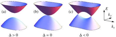
Figure 1: Evolution of the electron energy spectrum at the phase transition.

In the case of $\Delta<0$, the spectrum has two Dirac cones [Fig. 1(c)] located at $\mathbf{k}=(\pm K_{x},0)$ with $K_{x}=\sqrt{-\Delta/a}$. In the vicinity of these points, the linearized Hamiltonian (1) reads

$$H\simeq\pm v_{x}(k_{x}\mp K_{x})\sigma_{x}+vk_{y}\sigma_{y},$$ (4)

where the velocities $v_{x}=2\sqrt{-a\Delta}$ in the $x$ direction and $v$ in the $y$ direction are different in general. The spectrum has saddle points $E_{\mathbf{k}=0}^{\pm}=\pm|\Delta|$ with divergent density of states (the van Hove singularity).

The one-loop polarization function at finite temperature $T$ is given by

$$\Pi(i\omega_{m},\mathbf{q}) =g_{\rm s}T\sum_{n=-\infty}^{\infty}\int\frac{d^{2}k}{(2\pi)^{2}}\operatorname{Tr}\bigl{[}G(i\Omega_{n},\mathbf{k})$$

$$\quad\times G(i\Omega_{n}+i\omega_{m},\mathbf{k}+\mathbf{q})\bigr{]},$$ (5)

where $\omega_{m}=2\pi mT$, $\Omega_{n}=(2n+1)\pi T$ are the Matsubara frequencies, and the Green’s function is

$$G(i\Omega_{n},\mathbf{k})=\frac{i\Omega_{n}+\mu+(ak_{x}^{2}+\Delta)\sigma_{x}+vk_{y}\sigma_{y}}{(i\Omega_{n}+\mu)^{2}-(ak_{x}^{2}+\Delta)^{2}-v^{2}k_{y}^{2}}.$$ (6)

Evaluating the trace and the sum over $n$ yields

$$\Pi(i\omega_{m},\mathbf{q})=g_{\rm s}\!\int\!\!\frac{d^{2}k}{(2\pi)^{2}}\!\!\sum_{\lambda,\lambda^{\prime}=\pm}\!\!\!F^{\lambda,\lambda^{\prime}}_{\mathbf{k},\mathbf{k}+\mathbf{q}}\frac{n_{\rm F}(E_{\mathbf{k}}^{\lambda})-n_{\rm F}(E_{\mathbf{k}+\mathbf{q}}^{\lambda^{\prime}})}{E_{\mathbf{k}}^{\lambda}-E_{\mathbf{k}+\mathbf{q}}^{\lambda^{\prime}}+i\omega_{m}},$$ (7)

where $n_{\rm F}(x)=[e^{(x-\mu)/T}+1]^{-1}$ and

$$F^{\lambda,\lambda^{\prime}}_{\mathbf{k},\mathbf{k}^{\prime}}=\frac{1}{2}\biggl{[}1+\frac{(\Delta+ak_{x}^{2})(\Delta+ak_{x}^{\prime 2})+v^{2}k_{y}k_{y}^{\prime}}{E_{\mathbf{k}}^{\lambda}E_{\mathbf{k}^{\prime}}^{\lambda^{\prime}}}\biggr{]}$$ (8)

is the wave-function overlap factor. In the following, we consider only the case of $T=0$, when $n_{\rm F}(x)\to\theta(\mu-x)$ and the polarization function can be written as the sum of two terms,

$$\Pi(i\omega,\mathbf{q})=\Pi_{0}(i\omega,\mathbf{q})+\Pi_{1}(i\omega,\mathbf{q}),$$ (9)

where $\Pi_{0}(i\omega,\mathbf{q})$ is the “vacuum” polarization at $\mu=0$ and $\Pi_{1}(i\omega,\mathbf{q})$ gives an additional contribution when $\mu>\Delta$ (we choose $\mu\geqslant 0$, and the case $\mu<0$ is equivalent because of the electron-hole symmetry). These two terms are given by

$$\Pi_{0}(i\omega,\mathbf{q}) =-\chi_{\infty}^{-}(i\omega,\mathbf{q}),$$

$$\Pi_{1}(i\omega,\mathbf{q}) =\chi_{\mu}^{+}(i\omega,\mathbf{q})+\chi_{\mu}^{-}(i\omega,\mathbf{q}),$$ (10)

where

$$\chi_{\mu}^{\pm}(\omega,\mathbf{q})=g_{\rm s}\int\frac{d^{2}k}{(2\pi)^{2}}\sum_{\sigma=\pm}\frac{\theta(\mu-E^{+}_{\mathbf{k}})F^{+,\pm}_{\mathbf{k},\mathbf{k}+\mathbf{q}}}{E^{+}_{\mathbf{k}}-E^{\pm}_{\mathbf{k}+\mathbf{q}}+\sigma\omega}.$$ (11)

The $k_{y}$ integration in the above equation can be performed analytically for an arbitrary complex frequency $\omega$ away from the real axis (see Appendix A). The resulting expressions are

$$\begin{split}\Pi_{0}(\omega,\mathbf{q})&=-\frac{g_{\rm s}}{2\pi^{2}v(v^{2}q_{y}^{2}-\omega^{2})^{2}}\int\limits_{-\infty}^{\infty}dk_{x}\Biggl{[}v^{2}q_{y}^{2}(v^{2}q_{y}^{2}-\omega^{2})+\eta\xi(v^{2}q_{y}^{2}+\omega^{2})\operatorname{Re}\bigl{[}\operatorname{arctanh}(\xi/\eta)\bigr{]}\\ &\quad-\biggl{(}\xi^{2}\omega^{2}\frac{\sqrt{\alpha-\omega^{2}}}{\sqrt{\beta-\omega^{2}}}+v^{2}q_{y}^{2}\eta^{2}\frac{\sqrt{\beta-\omega^{2}}}{\sqrt{\alpha-\omega^{2}}}\biggr{)}\operatorname{arctanh}\frac{\sqrt{\min(\alpha,\beta)-\omega^{2}}}{\sqrt{\max(\alpha,\beta)-\omega^{2}}}\Biggr{]},\end{split}$$ (12)

$$\begin{split}\Pi_{1}(\omega,\mathbf{q})&=\frac{g_{\rm s}\theta(\mu-\Delta)}{4\pi^{2}v(v^{2}q_{y}^{2}-\omega^{2})^{2}}\int\limits_{-\sqrt{(\mu-\Delta)/a}}^{\sqrt{(\mu-\Delta)/a}}dk_{x}\theta(\mu+\Delta+ak_{x}^{2})\biggl{[}\eta\xi(v^{2}q_{y}^{2}+\omega^{2})\operatorname{arctanh}\frac{\widetilde{\mu}}{\mu}\\ &\quad-\biggl{(}\xi^{2}\omega^{2}\frac{\sqrt{\alpha-\omega^{2}}}{\sqrt{\beta-\omega^{2}}}+v^{2}q_{y}^{2}\eta^{2}\frac{\sqrt{\beta-\omega^{2}}}{\sqrt{\alpha-\omega^{2}}}\biggr{)}\operatorname{arctanh}\frac{\widetilde{\mu}(\eta\xi+v^{2}q_{y}^{2}-\omega^{2})-2vq_{y}(ak_{x}^{2}+\Delta)^{2}}{\mu\sqrt{\alpha-\omega^{2}}\sqrt{\beta-\omega^{2}}}\\ &\quad-2vq_{y}\eta\xi\omega\operatorname{arctanh}\frac{\eta\xi+v^{2}q_{y}^{2}-\omega^{2}+2vq_{y}\widetilde{\mu}}{2\mu\omega}+(q_{y}\to-q_{y})\biggr{]},\end{split}$$ (13)

where

$$\xi =aq_{x}(q_{x}+2k_{x}),$$

$$\eta =\xi+2(ak_{x}^{2}+\Delta),$$

$$\alpha =\eta^{2}+v^{2}q_{y}^{2},$$ (14)

$$\beta =\xi^{2}+v^{2}q_{y}^{2},$$

$$\widetilde{\mu} =\sqrt{\mu^{2}-(ak_{x}^{2}+\Delta)^{2}},$$

and the retarded polarization on the real $\omega$ axis is obtained using the prescription $\omega\to\omega+i0$. We use Eqs. (12) and (13) in our numerical calculations of the collective excitation spectrum and also to analytically obtain some important limits.

The imaginary part of the vacuum term can be calculated analytically (see Appendix B). If $\Delta<0$ and $q_{x}<2K_{x}$, it has a logarithmic singularity at $\omega=\pm\widetilde{\omega}$, where

$$\widetilde{\omega}=\sqrt{v^{2}q_{y}^{2}+a^{2}(2K_{x}^{2}-q_{x}^{2}/2)^{2}}.$$ (15)

In the vicinity of this singularity, $\operatorname{Im}\Pi_{0}(\omega,\mathbf{q})$ is given by (including terms finite at $\omega=\pm\widetilde{\omega}$)

$$\operatorname{Im}\Pi_{0}(\omega,q_{x},q_{y})\simeq\frac{\mp g_{\rm s}}{64\pi\sqrt{a}v}\Biggl{[}\frac{v^{2}q_{y}^{2}}{a^{3/2}\widetilde{q}^{3}}\ln\frac{512a^{2}\widetilde{q}^{6}}{\widetilde{\omega}|q_{x}^{2}-\widetilde{q}^{2}||\omega\mp\widetilde{\omega}|}$$

$$\quad-\frac{\widetilde{\omega}^{2}(q_{x}^{2}-3\widetilde{q}^{2})+v^{2}q_{y}^{2}(q_{x}^{2}+\widetilde{q}^{2})}{a^{3/2}q_{x}^{2}\widetilde{q}^{3}}$$ (16)

$$\quad+\frac{\widetilde{\omega}^{2}-8a^{2}(q_{x}^{4}+2q_{x}^{2}\widetilde{q}^{2}-\widetilde{q}^{4})}{a^{3/2}q_{x}^{3}}\ln\frac{|q_{x}-\widetilde{q}|}{q_{x}+\widetilde{q}}\Biggr{]},$$

where $\widetilde{q}=\sqrt{K_{x}^{2}/2-q_{x}^{2}/8}$. For $q_{x}=0$, this simplifies to

$$\operatorname{Im}\Pi_{0}(\omega,0,q_{y})\simeq\frac{\mp g_{\rm s}vq_{y}^{2}}{\pi\sqrt{a}(-8\Delta)^{3/2}}\biggl{(}\ln\frac{128\Delta^{2}}{\widetilde{\omega}_{0}|\omega\mp\widetilde{\omega}_{0}|}-\frac{8}{3}\biggr{)}$$ (17)

with $\widetilde{\omega}_{0}=\sqrt{4\Delta^{2}+v^{2}q_{y}^{2}}$. This logarithmic divergence for $\Delta<0$ is due to the van Hove singularity which results in the saddle point in the interband single-particle excitation (SPE) energy $E_{\mathbf{k}}^{+}-E_{\mathbf{k}+\mathbf{q}}^{-}$ [the real frequency corresponding to the pole of the integrand in Eq. (7)] as a function of $\mathbf{k}$ for a given external wave vector $\mathbf{q}$. A similar divergence of $\operatorname{Im}\Pi_{0}(\omega,\mathbf{q})$ due to the presence of the van Hove singularity appears in graphene stauber ; yuan . In contrast to the case of graphene, in our model this singularity occurs only at a single point in the momentum space between the two Dirac cones. Because of this, the divergent term is proportional to $q_{y}$ and vanishes for the momentum directed along the $x$ axis.

For $\Delta=0$, some limiting cases of vacuum polarization (12) can be evaluated analytically,

$$\Pi(\omega,q_{x}=0,q_{y})=-\frac{\Gamma(5/4)}{\Gamma(3/4)}\frac{g_{\rm s}vq_{y}^{2}}{6\sqrt{\pi a}(v^{2}q_{y}^{2}-\omega^{2})^{3/4}},$$ (18)

$$\Pi(\omega=0,q_{x},q_{y}=0)=-\frac{g_{\rm s}|q_{x}|}{16v},$$ (19)

in agreement with the previously reported results isobe ; cho .

III Plasmons

Plasmon dispersion $\omega_{\rm p}(\mathbf{q})$ in the RPA is obtained from zeros of the dielectric function

$$\epsilon(\omega,\mathbf{q})=1-V(\mathbf{q})\Pi(\omega,\mathbf{q}),$$ (20)

where $\Pi(\omega,\mathbf{q})$ is the one-loop polarization function and $V(\mathbf{q})=2\pi e^{2}/(\kappa q)$ is the Coulomb potential screened only by the substrate with the corresponding background dielectric constant $\kappa$.

We numerically found the real solutions $\omega=\omega_{\rm p}(\mathbf{q})$ of Eq. (20) in the regions where $\operatorname{Im}\Pi(\omega,\mathbf{q})=0$, i.e., the Landau damping is absent. For the SPE regions where the imaginary part of the polarization function is nonzero, we calculate the energy-loss function $-\operatorname{Im}[1/\epsilon(\omega,\mathbf{q})]$, the peaks of which represent the damped plasmons. Our approach assumes the strictly two-dimensional system and does not take into account the charge distribution in the perpendicular direction. Nevertheless, our results will be valid if the characteristic length of this distribution $l_{z}$ (e.g., the interlayer distance in the case of bilayer BP) is much smaller then $1/|\mathbf{q}|$ for the considered wave vectors $\mathbf{q}$.

In the case of $\mu=0$, there are no real solutions of Eq. (20) and the energy-loss function is shown in Fig. 2. For $\Delta<0$, the logarithmic divergence due to the van Hove singularity manifests itself as a dip in $-\operatorname{Im}[1/\epsilon(\omega,\mathbf{q})]$ for $q_{y}\neq 0$ and $\omega=\widetilde{\omega}$ followed by a peak at a larger energy [Fig. 2(b)]. Analogous behavior has also been reported in graphene yuan .

The evolution of the plasmon spectrum across the phase transition at nonzero chemical potential is shown in Fig. 3. The momentum is chosen to be aligned with one of the principal axes. In the case of $q_{y}=0$, the dielectric function (20) expressed in terms of the dimensionless momentum $q_{x}\sqrt{a/\mu}$ and energy $\omega/\mu$ depends only on a single adjustable parameter $\kappa v$. Similarly, $\epsilon(\omega,\mathbf{q})$ at $q_{x}=0$ can be represented as a function of the dimensionless momentum $q_{y}v/\mu$ and energy $\omega/\mu$, which depends on a single parameter $\kappa^{2}a\mu$. In our numerical calculations, we choose the values of the parameters $\kappa v=10^{-3}c\approx 3\times 10^{5}$ m/s, $a\mu=v^{2}/4$. The latter choice corresponds, e.g., to $m_{x}=1/(2a)=m_{\rm e}$ and $\mu\approx 0.26$ eV, where $m_{\rm e}$ is the bare electron mass.

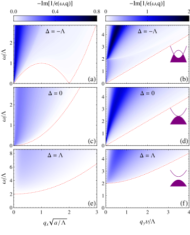
Figure 2: Energy-loss function $-\operatorname{Im}[1/\epsilon(\omega,\mathbf{q})]$ at $\mu=0$ for positive, zero, and negative $\Delta$. Left: $q_{y}=0$, $\kappa v=10^{-3}c$, and $\Lambda$ is an arbitrary energy scale. Right: $q_{x}=0$, $2\kappa\sqrt{a\mu}=10^{-3}c$, and $\kappa^{2}\Lambda=4\times 10^{-3}e^{2}/a$. The boundaries of the SPE regions are marked by dotted lines. The insets in the right panels schematically show the band structure and filling of the bands.

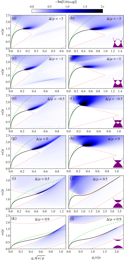
Figure 3: Energy-loss function $-\operatorname{Im}[1/\epsilon(\omega,\mathbf{q})]$ at $q_{y}=0$, $\kappa v=10^{-3}c$ (left) and $q_{x}=0$, $2\kappa\sqrt{a\mu}=10^{-3}c$ (right) for different values of $\Delta/\mu$. The undamped plasmon mode and its long-wavelength asymptote (23) are shown by solid and dashed lines, respectively. The boundaries of the SPE regions are marked by dotted lines. The insets in the right panels schematically show the band structure and filling of the bands.

In the regime $\sqrt{a}q_{x},vq_{y}\ll\omega\ll\mu$, i.e., relevant for the long-wavelength plasmons, the asymptotic behavior of the polarization function is

$$\Pi(\omega,\mathbf{q})=\frac{g_{\rm s}\sqrt{\mu}}{4\pi^{2}v\sqrt{a}\omega^{2}}\bigl{[}\mu aq_{x}^{2}f_{x}(\Delta/\mu)+v^{2}q_{y}^{2}f_{y}(\Delta/\mu)\bigr{]},$$ (21)

where the functions $f_{x,y}(\delta)$ are defined as

$$\begin{split}f_{x}(\delta)&=8\int_{t_{0}}^{1}dt\frac{t^{2}\sqrt{t-\delta}}{\sqrt{1-t^{2}}},\\ f_{y}(\delta)&=2\int_{t_{0}}^{1}dt\frac{\sqrt{1-t^{2}}}{\sqrt{t-\delta}},\end{split}$$ (22)

with $t_{0}=\max(\delta,-1)$ and shown in Fig. 4. The analytical expressions for $f_{x,y}(\delta)$ in terms of the complete elliptic integrals are given in Appendix C.

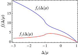
Figure 4: Factors $f_{x}(\Delta/\mu)$ and $f_{y}(\Delta/\mu)$ determining the long-wavelength plasmon dispersion (23).

Using Eq. (21), we obtain the long-wavelength plasmon dispersion,

$$\omega_{\rm p}(\mathbf{q}) \simeq\sqrt{\frac{g_{\rm s}e^{2}\mu q}{2\pi\kappa}}\biggl{[}\frac{\sqrt{\mu a}}{v}f_{x}(\Delta/\mu)\cos^{2}\theta$$

$$\quad+\frac{v}{\sqrt{\mu a}}f_{y}(\Delta/\mu)\sin^{2}\theta\biggr{]}^{1/2},$$ (23)

where $\cos\theta=q_{x}/q$, $\sin\theta=q_{y}/q$. It has the usual square-root dependence on the momentum just as expected for a 2D system, with the anisotropy of the spectrum being fully determined by the dimensionless factor $\sqrt{\mu a}/v$ and the two functions $f_{x,y}(\Delta/\mu)$. This undamped plasmon mode lies in the gap between the interband and the intraband SPE regions (Fig. 3).

For $-\Delta\gg\mu$, i.e., for well separated Dirac cones [Figs. 3(a) and 3(b)], using the asymptotics

$$\begin{split}f_{x}(\delta)&=4\pi|\delta|^{1/2}+\mathcal{O}(|\delta|^{-1/2}),\\ f_{y}(\delta)&=\pi|\delta|^{-1/2}+\mathcal{O}(|\delta|^{-3/2}),\qquad-\delta\gg 1,\end{split}$$ (24)

one can obtain the plasmon dispersion from Eq. (23) in this limit

$$\omega_{\rm p}(\mathbf{q})\simeq\sqrt{\frac{g_{\rm s}e^{2}\mu q}{\kappa}}\biggl{[}\frac{v_{x}}{v}\cos^{2}\theta+\frac{v}{v_{x}}\sin^{2}\theta\biggr{]}^{1/2}.$$ (25)

This result corresponds to the linearized Hamiltonian (4) and provides a generalization of the long-wavelength plasmon spectrum in a single-layer graphene shung to the case of the different Fermi velocities in the $x$ and $y$ direction.

When the Fermi level crosses the van Hove singularity at $|\mu|=-\Delta$ and the Fermi surfaces of the two Dirac cones merge into a single one [the plasmon spectrum at this transition is shown in Figs. 3(c) and 3(d)], the plasmon frequency in the long wavelengths changes continuously as a function of $\Delta/\mu$ but has a logarithmic singularity of its derivative, as seen in Fig. 4. The functions  (22) in the vicinity of this crossing are

$$\begin{split}f_{x}(-1+\varepsilon)&=2\sqrt{2}\bigl{(}\tfrac{56}{15}+\varepsilon\ln|\varepsilon|\bigr{)}+\mathcal{O}(\varepsilon),\\ f_{y}(-1+\varepsilon)&=\sqrt{2}\bigl{(}\tfrac{8}{3}-\varepsilon\ln|\varepsilon|\bigr{)}+\mathcal{O}(\varepsilon).\end{split}$$ (26)

For $\Delta<0$, there also exists an additional damped plasmon mode in the $x$ direction for momenta $0<q_{x}<2K_{x}$ with its maximum at $q_{x}\sim K_{x}$, which lies entirely in the intraband SPE region [Figs. 3(a), 3(c), and 3(e)].

At the crossing of the critical point $\Delta=0$ [Figs. 3(g) and 3(h)] the spectrum of the undamped plasmon changes smoothly and we have

$$\begin{split}f_{x}(0)&=3\sqrt{\pi}\,\Gamma(3/4)/\Gamma(9/4)\approx 5.751,\\ f_{y}(0)&=2\sqrt{\pi}\,\Gamma(5/4)/\Gamma(7/4)\approx 3.496,\end{split}$$ (27)

in agreement note with Ref. banerjee .

The effect of a small positive $\Delta/\mu$ is similar to that in the case of gapped graphene wang : the plasmon mode becomes extended to larger values of momenta due to the opening of the gap between the interband and intraband SPE continua [Figs. 3(i) and 3(j)]. In the regime $\Delta\to\mu$ [Figs. 3(k) and 3(l)], electrons have approximately parabolic anisotropic dispersion  (3). Using the asymptotic behavior of (22) for $\delta\to 1$,

$$\begin{split}f_{x}(1-\varepsilon)&=2\sqrt{2}\pi\varepsilon+\mathcal{O}(\varepsilon^{2}),\\ f_{y}(1-\varepsilon)&=\sqrt{2}\pi\varepsilon+\mathcal{O}(\varepsilon^{2}),\qquad 0\leqslant\varepsilon\ll 1,\end{split}$$ (28)

we recover from Eq. (23) in this limit,

$$\omega_{\rm p}(\mathbf{q})\simeq\sqrt{\frac{g_{\rm s}e^{2}\mu_{0}q}{\kappa}}\biggl{[}\sqrt{\frac{m_{y}}{m_{x}}}\cos^{2}\theta+\sqrt{\frac{m_{x}}{m_{y}}}\sin^{2}\theta\biggr{]}^{1/2},$$ (29)

as previously reported in Ref. rodin for the monolayer BP.

IV Conclusions

We have evaluated the polarization function and the spectrum of collective excitations in the two-dimensional system undergoing a topological phase transition with two merging Dirac points. A single integral representation for $\Pi(\omega,\mathbf{q})$ has been derived which is suitable for calculations on both real and imaginary frequency axes. An analytic expression was obtained for the imaginary part of the vacuum polarization and its asymptotic behavior near the logarithmic divergence due to the van Hove singularity. We analytically found the long-wavelength plasmon dispersion and numerically studied the spectrum of collective excitations for arbitrary momenta for both zero and nonzero values of the chemical potential. By evaluating the energy-loss function, we have found both undamped and damped plasmon excitations at zero temperature and studied their evolution across the merging transition. The presence of the van Hove singularity in the electron spectrum leads to the existence of the gapped damped plasmon mode at zero chemical potential in the semimetal phase. At finite $\mu$, there is one undamped anisotropic collective mode with the square-root dispersion, which lies in the gap between the interband and intraband SPE regions. In the gapped phase ($\Delta>0$), this undamped mode is generically extended to larger values of momenta due to the enhanced separation between the two SPE continua. At the critical point ($\Delta=0$), the undamped plasmon dispersion changes smoothly, while an additional damped and strongly anisotropic mode emerges at $\Delta<0$ in the interband SPE continuum. The crossing of van Hove singularity by the Fermi level manifests itself in a divergent derivative of the long-wavelength plasmon frequency.

Appendix A Calculation of the polarization function

The integrand in Eq. (11) can be written as

$$\sum_{\sigma=\pm}\frac{F^{+,\pm}_{\mathbf{k},\mathbf{k}+\mathbf{q}}}{E^{+}_{\mathbf{k}}-E^{\pm}_{\mathbf{k}+\mathbf{q}}+\sigma\omega}=\frac{\partial}{\partial k_{y}}\mathcal{F}_{\pm}(\omega,\mathbf{q},\mathbf{k}),$$ (30)

where

$$\mathcal{F}_{\pm}(\omega,\mathbf{q},\mathbf{k})=\frac{1}{2v(v^{2}q_{y}^{2}-\omega^{2})^{2}}\biggl{[}-v^{2}q_{y}\gamma(v^{2}q_{y}^{2}-\omega^{2})$$

$$\quad+\eta\xi(v^{2}q_{y}^{2}+\omega^{2})\operatorname{arctanh}\frac{2k_{y}-q_{y}}{\gamma}$$

$$\quad-2vq_{y}\eta\xi\omega\operatorname{arctanh}\frac{\eta\xi-\omega^{2}+2v^{2}q_{y}k_{y}}{v\gamma\omega}$$

$$\quad-\biggl{(}\xi^{2}\omega^{2}\frac{\sqrt{\alpha-\omega^{2}}}{\sqrt{\beta-\omega^{2}}}+v^{2}q_{y}^{2}\eta^{2}\frac{\sqrt{\beta-\omega^{2}}}{\sqrt{\alpha-\omega^{2}}}\biggr{)}$$

$$\quad\times\operatorname{arctanh}\frac{(2k_{y}-q_{y})(\eta\xi+v^{2}q_{y}^{2}-\omega^{2})-q_{y}(\eta-\xi)^{2}}{\gamma\sqrt{\alpha-\omega^{2}}\sqrt{\beta-\omega^{2}}}$$

$$\quad\mp\bigl{(}q_{y}\to-q_{y},\;\xi\to-\xi\bigr{)}\biggr{]},$$ (31)

variables $\eta$, $\xi$, $\alpha$, $\beta$ are defined in Eq. (14) and

$$\gamma=\sqrt{(\eta-\xi)^{2}/v^{2}+(2k_{y}-q_{y})^{2}}.$$ (32)

The function $\mathcal{F}_{\pm}(\omega,\mathbf{q},\mathbf{k})$ does not have any singularities for $\operatorname{Im}\omega\neq 0$ and the multivalued functions taken on their principal branches. Therefore, the definite $k_{y}$ integral of (30) is obtained straightforwardly by evaluating $\mathcal{F}_{\pm}(\omega,\mathbf{q},\mathbf{k})$ in the integration limits, which, after some algebra, yields Eqs. (12) and (13).

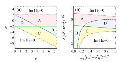
Figure 5: Regions (36) plotted for parameters (a) $\phi$ and $\psi$ or (b) $\mathbf{q}$, $\omega$, and $\Delta$. At the boundaries, $\operatorname{Im}\Pi_{0}(\omega,\mathbf{q})$ has a logarithmic singularity (solid line), logarithmically divergent derivative (dashed line) or jump discontinuity of the derivative (dotted line).

Appendix B Analytic expression for $\operatorname{Im}\Pi_{0}(\omega,\mathbf{q})$

The nonzero imaginary part of the expressions (12) and (13) for the polarization function originates from the regions where the argument of inverse hyperbolic tangent is real and larger than unity,

$$\operatorname{Im}\bigl{[}\operatorname{arctanh}(x\pm i0)\bigr{]}=\pm\frac{\pi}{2}\theta(x^{2}-1).$$ (33)

The step function above determines the integration limits which, for the nonvacuum term (13), involves the roots of the higher-order polynomials that cannot be written in a closed form in the general case (for nonzero $q_{x}$, $q_{y}$, and $\Delta$). For the vacuum term, on the other hand, the imaginary part can be evaluated in terms of the complete elliptic integrals table :

$$\begin{split}&\operatorname{Im}\Pi_{0}(\omega,q_{x},q_{y})=-\frac{g_{\rm s}\sqrt{|\omega|}\,\theta(1-\tau)\theta(2-\psi)\theta(\nu)}{128\pi\sqrt{a}v(1-\tau)^{3/4}}\\ &\quad\times\operatorname{sgn}(\omega)\biggl{\{}4(2\psi+3\varphi-\tau\varphi+2\tau\psi)h_{i}E(t_{i})\\ &\quad+(1-b)h_{i}^{-1}\Bigl{[}r_{i}K(t_{i})+s_{i}\bigl{(}(16-4\psi\varphi)(1-\tau)\\ &\quad-\varphi^{2}(3-\tau)\bigr{)}\Pi(\pi/2,\rho_{i},t_{i})\Bigr{]}\biggr{\}},\end{split}$$ (34)

where

$$d =4\Delta(\omega^{2}-v^{2}q_{y}^{2})^{-1/2}, \tau=v^{2}q_{y}^{2}/\omega^{2},$$

$$\varphi =(\omega^{2}-v^{2}q_{y}^{2})^{1/2}/(aq_{x}^{2}), \psi=d+1/\varphi,$$ (35)

$$\nu =(\psi+\varphi+2)/4, b=(2-\psi)/\varphi,$$

and the subscript $i=\mathrm{A},\mathrm{B},\mathrm{C},\mathrm{D}$ determines the region in the ($\varphi,\psi$) space (see Fig. 5):

$$\begin{split}\mathrm{A}:\qquad&-2<\psi<2,\quad\varphi>2-\psi,\\ \mathrm{B}:\qquad&\psi<-2,\quad\varphi>2-\psi,\\ \mathrm{C}:\qquad&\psi<-2,\quad-2-\psi<\varphi<2-\psi,\\ \mathrm{D}:\qquad&-2<\psi<2,\quad 0<\varphi<2-\psi,\end{split}$$ (36)

and

$$\begin{split}&\rho_{\mathrm{A}}=\rho_{\mathrm{D}}^{-1}=b,\qquad\rho_{\mathrm{C}}=\rho_{\mathrm{B}}^{-1}=\nu,\\ &t_{\mathrm{A}}=t_{\mathrm{C}}=t_{\mathrm{B}}^{-1}=t_{\mathrm{D}}^{-1}=\sqrt{b\nu},\\ &s_{\mathrm{C}}=s_{\mathrm{D}}=1,\qquad s_{\mathrm{A}}=s_{\mathrm{B}}=-1,\\ &h_{\mathrm{A}}=h_{\mathrm{C}}=1,\qquad h_{\mathrm{B}}=h_{\mathrm{D}}=\sqrt{b\nu},\\ &r_{\mathrm{A}}=-\varphi\bigl{[}12+4\psi+3\varphi-\tau(4+4\psi+\varphi)\bigr{]},\\ &r_{\mathrm{B}}=4\nu\bigl{[}2\psi-3\varphi+\tau(2\psi+\varphi)\bigr{]},\\ &r_{\mathrm{C}}=-4\bigl{[}4+3\varphi-\tau(4+\varphi)\bigr{]},\\ &r_{\mathrm{D}}=(\psi-2)(8+2\psi+3\varphi)\\ &\qquad+\tau[\psi(4+2\psi-\varphi)+2(8+\varphi)].\end{split}$$ (37)

For $q_{x}=0$, only regions A and B survive and Eq. (34) simplifies to

$$\begin{split}&\operatorname{Im}\Pi_{0}(\omega,0,q_{y})=-\frac{g_{\rm s}\tau\sqrt{|\omega|}\theta(1-\tau)\theta(2-d)\operatorname{sgn}(\omega)}{12\pi\sqrt{a}v(1-\tau)^{3/4}}\\ &\;\times\!\left\{\begin{array}[]{ll}(1-d)K(\widetilde{u})+2dE(\widetilde{u}),&|d|<2,\vskip 6.0pt plus 2.0pt minus 2.0pt\\ \dfrac{2+d^{2}}{2\widetilde{u}}K(1/\widetilde{u})+\dfrac{d(2-d)}{2\widetilde{u}}E(1/\widetilde{u}),&d<-2,\end{array}\right.\end{split}$$ (38)

where $\widetilde{u}=\sqrt{2-d}/2$.

Appendix C Expressions for $f_{x,y}(\Delta/\mu)$

The functions (22) determining the long-wavelength plasmon frequency can be written in terms of the complete elliptic integrals as

$$f_{x}(\delta) =\frac{8\sqrt{2}}{15}\left\{\begin{array}[]{ll}2(9-2\delta^{2})E(u)-(1+\delta)(9-2\delta)K(u),&|\delta|<1,\vskip 6.0pt plus 2.0pt minus 2.0pt\\ 2u\bigl{[}(9-2\delta^{2})E(1/u)+2\delta(1+\delta)K(1/u)\bigr{]},&\delta<-1,\end{array}\right.$$ (41)

$$f_{y}(\delta) =\frac{4\sqrt{2}}{3}\left\{\begin{array}[]{ll}(1+\delta)K(u)-2\delta E(u),&|\delta|<1,\vskip 6.0pt plus 2.0pt minus 2.0pt\\ 2u\bigl{[}(1+\delta)K(1/u)-\delta E(1/u)\bigr{]},&\delta<-1,\end{array}\right.$$ (44)

where $u=\sqrt{(1-\delta)/2}$. According to the notations used in Ref. adroguer ,

$$f_{x}(\delta)=4\,\mathcal{I}_{3}(0,\delta),\qquad f_{y}(\delta)=\mathcal{I}_{2}(0,\delta).$$ (45)

References

- (1) Physics of Graphene, edited by H. Aoki and M. S. Dresselhaus (Springer, New York, 2014).
- (2) D. S. L. Abergel, V. Apalkov, J. Berashevich, K. Ziegler, and T. Chakraborty, Adv. Phys. 59, 261 (2010).
- (3) J. Wang, S. Deng, Z. Liu and Z. Liu, Nat. Sci. Rev. 2, 22 (2015) [arXiv: 1410.5895].
- (4) T. Chakraborty and V. Apalkov, in graphene_book , Chap. 8; Solid State Commun. 175–176, 123 (2013) [arXiv: 1302.2940]; T. Chakraborty and P. Pietiläinen, Phys. Rev. Lett. 76, 4018 (1996); Phys. Rev. B 39, 7971 (1989); D. S. L. Abergel and T. Chakraborty, Phys. Rev. Lett. 102, 056807 (2009) [arXiv: 0811.0574]; V. M. Apalkov and T. Chakraborty, ibid. 97, 126801 (2006) [arXiv: cond-mat/0606037]; 105, 036801 (2010) [arXiv: 1007.4188]; 107, 186803 (2011) [arXiv: 1104.2020].
- (5) D. Langbein, Phys. Rev. 180, 633 (1969); D. R. Hofstadter, Phys. Rev. B 14, 2239 (1976); L. A. Ponomarenko, R. V. Gorbachev, G. L. Yu, D. C. Elias, R. Jalil, A. A. Patel, A. Mishchenko, A. S. Mayorov, C. R. Woods, J. R. Wallbank, M. Mucha-Kruczynski, B. A. Piot, M. Potemski, I. V. Grigorieva, K. S. Novoselov, F. Guinea, V. I. Fal’ko, and A. K. Geim, Nature 497, 594 (2013) [arXiv: 1212.5012]; B. Hunt, J. D. Sanchez-Yamagishi, A. F. Young, M. Yankowitz, B. J. LeRoy, K. Watanabe, T. Taniguchi, P. Moon, M. Koshino, P. Jarillo-Herrero, and R. C. Ashoori, Science 340, 1427 (2013) [arXiv: 1303.6942]; C. R. Dean, L. Wang, P. Maher, C. Forsythe, F. Ghahari, Y. Gao, J. Katoch, M. Ishigami, P. Moon, M. Koshino, T. Taniguchi, K. Watanabe, K. L. Shepard, J. Hone, and P. Kim, Nature 497, 598 (2013) [arXiv: 1212.4783].
- (6) V. M. Apalkov and T. Chakraborty, Phys. Rev. Lett. 112, 176401 (2014) [arXiv: 1311.4935]; A. Ghazaryan and T. Chakraborty, Phys. Rev. B 91, 125131 (2015) [arXiv: 1412.2792]; A. Ghazaryan, T. Chakraborty, and P. Pietiläinen, J. Phys.: Condens. Matter 27, 185301 (2015) [arXiv: 1408.3424]; A. Ghazaryan and T. Chakraborty, Phys. Rev. B 92, 235404 (2015) [arXiv: 1502.01373].
- (7) P. De Padova, C. Ottaviani, C. Quaresima, B. Olivieri, P. Imperatori, E. Salomon, T. Angot, L. Quagliano, C. Romano, A. Vona, M. Muniz-Miranda, A. Generosi, B. Paci, and G. Le Lay, 2D Mater. 1, 021003 (2014); J. Sone, T. Yamagami, Y. Aoki, K. Nakatsuji, and H. Hirayama, New J. Phys. 16, 095004 (2014); M. E. Dávila, L. Xian, S. Cahangirov, A. Rubio and G. Le Lay, New J. Phys. 16, 095002 (2014) [arXiv: 1406.2488].
- (8) V. M. Apalkov and T. Chakraborty, Phys. Rev. B 90, 245108 (2014) [arXiv: 1407.4441]; 91, 235447 (2015) [arXiv: 1504.01749].
- (9) W. Luo and T. Chakraborty, Phys. Rev. B 92, 155123 (2015) [arXiv: 1506.07896].
- (10) Xi Ling, H. Wang, S. Huang, F. Xia, and M. S. Dresselhaus, PNAS 112, 4523 (2015) [arXiv: 1503.08367]; H. Liu, Y. Du, Y. Deng and P. D. Ye, Chem. Soc. Rev. 44, 2732 (2015) [arXiv: 1411.0056].
- (11) A. Ghazaryan and T. Chakraborty, Phys. Rev. B 92, 165409 (2015) [arXiv: 1507.04709].
- (12) A. Tsukazaki, A. Ohtomo, T. Kita, Y. Ohno, H. Ohno, and M. Kawasaki, Science 315, 1388 (2007); A. Tsukazaki, S. Akasaka, K. Nakahara, Y. Ohno, H. Ohno, D. Maryenko, A. Ohtomo, and M. Kawasaki, Nat. Mater. 9, 889 (2010); J. Falson, D. Maryenko, B. Friess, D. Zhang, Y. Kozuka, A. Tsukazaki, J.H. Smet and M. Kawasaki, Nat. Phys. 11, 347 (2015).
- (13) W. Luo and T. Chakraborty, arXiv: 1512.05815.
- (14) Y. Hasegawa, R. Konno, H. Nakano, and M. Kohmoto, Phys. Rev. B 74, 033413 (2006) [arXiv: cond-mat/0604433].
- (15) S.-L. Zhu, B. Wang, and L.-M. Duan, Phys. Rev. Lett. 98, 260402 (2007) [arXiv: cond-mat/0703454].
- (16) B. Wunsch, F. Guinea, and F. Sols, New J. Phys. 10, 103027 (2008) [arXiv: 0807.4245].
- (17) G. Montambaux, F. Piéchon, J.-N. Fuchs, and M. O. Goerbig, Phys. Rev. B 80, 153412 (2009) [arXiv: 0904.2117]; Eur. Phys. J. B 72, 509 (2009) [arXiv: 0907.0500].
- (18) V. M. Pereira, A. H. Castro Neto, and N. M. R. Peres, Phys. Rev. B 80, 045401 (2009) [arXiv: 0811.4396].
- (19) Q. Liu, X. Zhang, L. B. Abdalla, A. Fazzio, and A. Zunger, Nano Lett. 15, 1222 (2015) [arXiv: 1411.3932].
- (20) K. Dolui and S. Y. Quek, Sci. Rep. 5, 11699 (2015) [arXiv: 1503.03647].
- (21) J. M. Pereira and M. I. Katsnelson, Phys. Rev. B 92, 075437 (2015) [arXiv: 1504.02452]; A. N. Rudenko, S. Yuan, and M. I. Katsnelson, Phys. Rev. B 92, 085419 (2015) [arXiv: 1506.01954].
- (22) S. S. Baik, K. S. Kim, Y. Yi, and H. J. Choi, Nano Lett. 15, 7788 (2015) [arXiv: 1508.04932].
- (23) V. Pardo and W. E. Pickett, Phys. Rev. Lett. 102, 166803 (2009) [arXiv: 0903.4820]; Phys. Rev. B 81, 035111 (2010) [arXiv: 0910.4411]; S. Banerjee, R. R. P. Singh, V. Pardo, and W. E. Pickett, Phys. Rev. Lett. 103, 016402 (2009) [arXiv: 0906.1564].
- (24) H. Huang, Z. Liu, H. Zhang, W. Duan, and D. Vanderbilt, Phys. Rev. B 92, 161115 (2015) [arXiv: 1507.01742].
- (25) L. Tarruell, D. Greif, T. Uehlinger, G. Jotzu, and T. Esslinger, Nature 483, 302 (2012) [arXiv: 1111.5020]; L.-K. Lim, J.-N. Fuchs, and G. Montambaux, Phys. Rev. Lett. 108, 175303 (2012) [arXiv: 1201.1479].
- (26) M. C. Rechtsman, Y. Plotnik, J.M. Zeuner, D. Song, Z. Chen, A. Szameit, and M. Segev, Phys. Rev. Lett. 111, 103901 (2013) [arXiv: 1211.5683].
- (27) M. Bellec, U. Kuhl, G. Montambaux, and F. Mortessagne, Phys. Rev. Lett. 110, 033902 (2013) [arXiv: 1210.4642].
- (28) J. Kim, Seung S. Baik, S. H. Ryu, Y. Sohn, S. Park, B.-G. Park, J. Denlinger, Y. Yi, H. J. Choi, and K. S. Kim, Science 349, 723 (2015) [arXiv: 1508.05523].
- (29) P. Dietl, F. Piéchon, and G. Montambaux, Phys. Rev. Lett. 100, 236405 (2008) [arXiv: 0707.0219]; P. Delplace and G. Montambaux, Phys. Rev. B 82, 035438 (2010) [arXiv: 1001.3952].
- (30) S. Yuan, M. I. Katsnelson, and R. Roldán, arXiv: 1512.06345.
- (31) D. Carpentier, A. A. Fedorenko, and E. Orignac, Europhys. Lett. 102, 67010 (2013) [arXiv: 1303.4320].
- (32) H. Isobe, B.-J. Yang, A. Chubukov, J. Schmalian, and N. Nagaosa, Phys. Rev. Lett. 116, 076803 (2016) [arXiv: 1508.03781].
- (33) G. Y. Cho and E.-G. Moon, Sci. Rep. 6, 19198 (2016) [arXiv: 1508.03777].
- (34) P. Adroguer, D. Carpentier, G. Montambaux, and E. Orignac, arXiv: 1511.00036.
- (35) S. Banerjee and W. E. Pickett, Phys. Rev. B 86, 075124 (2012) [arXiv: 1207.5760].
- (36) T. Low, R. Roldán, H. Wang, F. Xia, P. Avouris, L. M. Moreno, and F. Guinea, Phys. Rev. Lett. 113, 106802 (2014) [arXiv: 1404.4035].
- (37) A. S. Rodin and A. H. Castro Neto, Phys. Rev. B 91, 075422 (2015) [arXiv: 1412.0811].
- (38) F. Jin, R. Roldán, M. I. Katsnelson, and S. Yuan, Phys. Rev. B 92, 115440 (2015) [arXiv: 1507.07013].
- (39) A. N. Rudenko and M. I. Katsnelson, Phys. Rev. B 89, 201408 (2014) [arXiv: 1404.0618].
- (40) T. Stauber, J. Schliemann, and N. M. R. Peres, Phys. Rev. B 81, 085409 (2010) [arXiv: 0910.1242].
- (41) S. Yuan, R. Roldán, and M. I. Katsnelson, Phys. Rev. B 84, 035439 (2011) [arXiv: 1103.5350].
- (42) Kenneth W.-K. Shung, Phys. Rev. B 34, 979 (1986); E. H. Hwang and S. Das Sarma, ibid. 75, 205418 (2007) [arXiv: cond-mat/0610561]; B. Wunsch, T. Stauber, F. Sols, and F. Guinea, New J. Phys. 8, 318 (2006) [arXiv: cond-mat/0610630].
- (43) According to the notations of Ref. banerjee , , .
- (44) X.-F. Wang and T. Chakraborty, Phys. Rev. B 75, 033408 (2007) [arXiv: cond-mat/0605498]; 75, 041404 (2007) [arXiv: cond-mat/0611635]; 81, 081402 (2010) [arXiv: 1001.2762]; P. K. Pyatkovskiy, J. Phys.: Condens. Matter 21, 025506 (2009) [arXiv: 0808.0931].
- (45) I. Gradshteyn and I. Ryzhik, Table of Integrals, Series, and Products, 7th ed. (Academic, New York, 2007).