Systematic Measures of Biological Networks, Part II: Degeneracy, Complexity and Robustness

Abstract.

This paper is Part II of a two-part series devoting to the study of systematic measures in a complex bio-network modeled by a system of ordinary differential equations. In this part, we quantify several systematic measures of a biological network including degeneracy, complexity and robustness. We will apply the theory of stochastic differential equations to define degeneracy and complexity for a bio-network. Robustness of the network will be defined according to the strength of attractions to the global attractor. Based on the study of stationary probability measures and entropy made in Part I of the series, we will investigate some fundamental properties of these systematic measures, in particular the connections between degeneracy, complexity and robustness.

1. Introduction

Consider a biological network modeled by the following system of ordinary differential equations (ODE system for short):

(1.1) $$x^{\prime}=f(x),\;\;\;x\in{\mathbb{R}}^{n},$$

where $f$ is a $C^{1}$ vector field on ${\mathbb{R}}^{n}$, called drift field. Adopting the idea of activating the functional connections among modules of the network via external noises in the case of neural systems [30, 23], we add additive white noise perturbations $\sigma dW_{t}$ to (1.1) to obtain the following system of stochastic differential equations (SDE system for short):

(1.2) $$\mathrm{d}X=f(X)\mathrm{d}t+\epsilon\sigma(x)\mathrm{d}W_{t},\;\;\;X\in{\mathbb{R}}^{n},$$

where $W_{t}$ is the standard $m$-dimensional Brownian motion, $\epsilon$ is a small parameter lying in an interval $(0,\epsilon^{*})$, and $\sigma$, called an noise matrix, is an $n\times m$ matrix-valued, bounded, $C^{1}$ function on ${\mathbb{R}}^{n}$ for some positive integer $m\geq n$, such that $\sigma(x)\sigma^{\top}(x)$ is everywhere non-singular. We denote the collection of such noise matrices by $\Sigma$. Under certain dissipation conditions, the SDE system (1.2) generates a diffusion process in ${\mathbb{R}}^{n}$ with well-defined transition probability kernel, and moreover, if the transition probability kernel admits a density function $p^{t}(\xi,x)$, then its time evolution $u(x,t)=\int_{\mathbb{R}^{n}}p^{t}(z,x)\xi(z)\mathrm{d}z$ satisfies the Fokker-Planck equation (FPE for short):

(1.3) $$\left\{\begin{array}[]{l}\frac{\partial u(x,t)}{\partial t}=\frac{1}{2}{{\epsilon}^{2}}\sum\limits_{i,j=1}^{n}{\partial_{ij}(a_{ij}(x)u(x))-\sum_{i=1}^{n}\partial_{i}(f(x)u(x))}:=L_{\epsilon}u(x),\\ \int_{{\mathbb{R}}^{n}}u(x)\rm dx=1,\end{array}\right.$$

where $(a_{ij}(x)):=A(x):=\sigma(x){{\sigma}^{\top}}(x)$. Denote

$$\mathcal{L}_{\epsilon}=\frac{1}{2}\epsilon^{2}\sum_{i,j=1}^{n}a_{ij}(x)\partial_{ij}+\sum_{i=1}^{n}f_{i}(x)\partial_{i}$$

as the adjoint of Fokker-Planck operator. If $u(x)$ is a weak stationary solution of (1.3), i.e., $u$ is a strictly positive, continuous function on ${\mathbb{R}}^{n}$ with $\int_{{\mathbb{R}}^{n}}u(x){\rm d}x=1$ such that

(1.4) $$\int_{{\mathbb{R}}^{n}}\mathcal{L}_{\epsilon}h(x)u(x)\mathrm{d}x=0,\qquad\;\forall h\in C_{0}^{\infty}(\mathbb{R}^{n}),$$

then the probability measure $\mu_{\epsilon}(\rm dx)=u(x)\mathrm{d}x$ is clearly a stationary measure of (1.3), i.e.,

(1.5) $$\int_{{\mathbb{R}}^{n}}\mathcal{L}_{\epsilon}h(x)\mu_{\epsilon}(\mathrm{d}x)=0,\qquad\;\forall h\in C_{0}^{\infty}(\mathbb{R}^{n}).$$

Conversely, it follows from the regularity theory of stationary measures [6] that any stationary measure of (1.3) must admit a density function which is necessarily a weak stationary solution of (1.3). We remark that an invariant probability measure of the diffusion process generated from SDE (1.2) must be a stationary measure of the FPE (1.3) and vice versa under some conditions.

In Part I of the series, we have assumed the following conditions:

• System (1.1) is dissipative and there exists a strong Lyapunov function $W(x)$ with respect to an isolating neighborhood $\mathcal{N}$ of the global attractor $\mathcal{A}$ such that

  $$W(x)\geq L_{1}\mathrm{dist}^{2}(x,\mathcal{A}),\;\;x\in\mathcal{N}$$

  for some $L_{1}>0$.

• For each $\epsilon\in(0,\epsilon^{*})$, the Fokker-Planck equation (1.3) admits a unique stationary probability measure $\mu_{\epsilon}$ such that for an isolating neighborhood $\mathcal{N}$ of $\mathcal{A}$,

  $$\lim_{\epsilon\rightarrow 0}\frac{\mu_{\epsilon}(\mathbb{R}^{n}\setminus\mathcal{N})}{\epsilon^{2}}=0,$$

  and moreover, there are constants $p,R_{0}>0$ such that

  $$\mu_{\epsilon}(\{x\,:\,|x|>r\})\leq e^{-\frac{r^{p}}{\epsilon^{2}}}$$

  for all $r>R_{0}$ and all $\epsilon\in(0,\epsilon^{*})$.

The desired concentration in H¹) can follow from various conditions, such as the existence of a quasi-potential function or a suitable Lyapunov function. See Part I of the series and Proposition 2.1 below for more information in this regard.

For each given $\epsilon\in(0,\epsilon^{*})$, the mutual information $MI(X_{1};X_{2})$ among any two modules (coordinate subspaces) $X_{1},X_{2}$ can be defined using the margins $\mu_{1}$, $\mu_{2}$ of $\mu_{\epsilon}$ with respect to $X_{1},X_{2}$, respectively. Such mutual information can then be used to quantify degeneracy and complexity. Inspired by [30], we will define the $\{\epsilon,\sigma\}$-degeneracy and -complexity of the evolutionary network (1.1) associated with $\sigma$ as an averaged combinations of certain mutual informations between different modules. Let $\{I,\mathcal{O}\}$ be a pair of coordinate subspaces of the variable set ${\mathbb{R}}^{n}$ which decompose ${\mathbb{R}}^{n}$, called an input-output pair. For any $0\leq k\leq|I|$, where $|I|$ denotes the dimension of the input space $I$, the degeneracy $D_{\epsilon}(I_{k})$ and complexity $C_{\epsilon}(I_{k})$, associated with the $k$-decomposition $I=I_{k}\cup I_{k}^{c}$ is defined as

$$D_{\epsilon}(I_{k})=MI(I;{{I}_{k}};\mathcal{O})=MI({{I}_{k}};\mathcal{O})+MI(I_{k}^{c};\mathcal{O})-MI(I;\mathcal{O})$$

and

$$C_{\epsilon}(I_{k})=MI({{I}_{k}};I_{k}^{c})\,,$$

where $I_{k}$ is a $k$-dimension subspace of $I$ spanned by $k$ variables. The degeneracy $D_{\epsilon}(\mathcal{O})$, respectively complexity $C_{\epsilon}(\mathcal{O})$, with respect to the input-output pair $\{I,\mathcal{O}\}$ is simply the average of all $D_{\epsilon}(I_{k})$’s, respectively all $C_{\epsilon}(I_{k})$’s. The degeneracy, respectively complexity, of the network (1.1) associated with $\sigma$, is then defined as $\mathcal{D}_{\sigma}=\liminf_{\epsilon\rightarrow 0}\sup_{\mathcal{O}}D_{\epsilon}(\mathcal{O})$, respectively $\mathcal{C}_{\sigma}=\liminf_{\epsilon\rightarrow 0}\sup_{\mathcal{O}}C_{\epsilon}(\mathcal{O})$. We refer the readers to Section 3 for details.

Another systematic measure for the network (1.1) is the robustness, which will be defined in Section  4 relevant to the strength of its global attractor, either in a uniform way or in an average way. As suggested in [21, 20], the robustness is not always equivalent to the stability. As to be seen in Section  4, if the performance function of the network (1.1) is known, then one can also define its functional robustness.

Many simulations and experiments have already suggested that there are close connections among degeneracy, complexity and robustness in a biological system (see e.g. [10, 29, 33, 32, 7]). For the evolutionary network (1.1) and its noise perturbation (1.2), we will rigorously show the following results under the conditions H⁰) and H¹) :

1. With respect to a fixed $\sigma\in\Sigma$, high degeneracy always yields high complexity (Theorem  5.1).

2. A robust system with non-degenerate attractor has positive degeneracy with respect to any $\sigma\in\Sigma$ (Theorem  5.2).

3. A robust system with stable equilibrium has positive degeneracy with respect to any $\sigma\in\Sigma$ under certain algebraic conditions (Theorem  5.4).

As in [10] for neural systems, results above are useful in characterizing degenerate biological networks in connection with their system complexities. This series of papers serves as a mathematical supplement of [23]. We refer readers to [23] for degeneracy, complexity, and robustness in biological models and discussions in this regard. Examples in [23] include a signaling pathway network and a population model.

The paper is organized as follows. Section 2 is a preliminary section. Section 3 defines degeneracy and complexity. The robustness is investigated in Section 4. Finally, the connection between degeneracy, complexity and robustness are proved in Section 5.

2. Preliminary

2.1. Existence and concentration of stationary measures

It was shown in Part I of the series [24] that the condition H¹) is implied by H⁰) together with the following condition:

• There is a positive function $U\in C^{2}({\mathbb{R}}^{n}\setminus\mathcal{A})$ satisfying the following properties:

  • $\lim_{|x|\to\infty}U(x)=\infty$;

  • There exists a constant $\rho_{m}>0$ such that $U$ is a uniform Lyapunov function of the family (1.3) of class ${\mathcal{B}}^{*}$ in ${\mathcal{N}}_{\infty}=:\mathbb{R}^{n}\setminus\Omega_{\rho_{m}}(U)$, i.e., there is a constant $\gamma>0$ independent of $\epsilon$ such that

    $$\mathcal{L}_{\epsilon}U(x)<-\gamma,\;\qquad x\in{\mathcal{N}}_{\infty}$$

    for all $\epsilon\in(0,\epsilon^{*})$. Moreover, a function $H(\rho)\in L^{1}_{loc}([\rho_{m},\infty))$ and constants $p>0$, $R>\rho_{m}$ exist such that

    $$H(\rho)\geq|\nabla U(x)|^{2},\quad x\in\Gamma_{\rho}(U),$$

    $$\int_{\rho_{m}}^{\rho}\frac{1}{H(s)}\mathrm{d}s\geq|x|^{p},\quad x\in\Gamma_{\rho}(U)$$

    for all $\rho>R$;

  • There exists a constant $\bar{\rho}_{m}\in(0,\rho_{m})$ such that $U$ is a uniform weak Lyapunov function of the family (1.3) in ${\mathcal{N}}_{*}=:{\mathbb{R}}^{n}\setminus{\mathcal{N}}_{\infty}\setminus\Omega_{\bar{\rho}_{m}}(U)$, i.e.,

    $$\mathcal{L}_{\epsilon}U(x)\leq 0,\;\qquad x\in{\mathcal{N}}_{*}$$

    for all $\epsilon\in(0,\epsilon^{*})$;

  • $\nabla U(x)\neq 0$, $x\in{\mathbb{R}}^{n}\setminus\Omega_{\bar{\rho}_{m}}(U)$;

  • $\Omega_{\bar{\rho}_{m}}(U)\subset{\mathcal{N}}$.

  In the above, ${\mathcal{L}}_{\epsilon}$, $\epsilon\in(0,\epsilon^{*})$, is the adjoint Fokker-Planck operator and $\Gamma_{\rho}$, $\Omega_{\rho}(U)$ denote the $\rho$-level set, $\rho$-sublevel set of $U$ for each $\rho>0$ respectively.

In summary, we have the following result.

Proposition 2.1.

(Corollary 3.1, [24] ) Conditions H⁰), H²) imply H¹).

Theorem 2.1.

(Theorem 3.1, [24]) If both H⁰) and H¹) hold, then for any $0<\delta\ll 1$ there exist constants $\epsilon_{0},M>0$ such that

$$\mu_{\epsilon}(B(\mathcal{A},M\epsilon))\geq 1-\delta,$$

whenever $\epsilon\in(0,\epsilon_{0})$.

Theorem 2.2.

(Theorem 3.3, [24]) Let

$$V(\epsilon)=\int_{\mathbb{R}^{n}}\mathrm{dist}^{2}(x,\mathcal{A})\mu_{\epsilon}(\mathrm{d}x)\,.$$

If both H⁰) and H¹) hold, then there are constants $V_{1},V_{2},\epsilon_{0}>0$ such that

$$V_{2}\epsilon^{2}\leq V(\epsilon)\leq V_{1}(\epsilon)\ ,\quad\epsilon\in(0,\epsilon_{0})\,.$$

Let $\mu$ be the probability measure with density $u$, define the differential entropy by

$$\mathcal{H}(\mu)=-\int_{\mathbb{R}^{n}}u(x)\log u(x)\mathrm{d}x\,.$$

Theorem 2.3.

(Theorem 4.1, [24]) Assume that H⁰) and H¹) hold. If $\mathcal{A}$ is a regular set, then

(2.1) $$\liminf_{\epsilon\rightarrow 0}\frac{\mathcal{H}(\mu_{\epsilon})}{\log\epsilon}\geq n-d\,,$$

where $d$ is the Minkowski dimension of $\mathcal{A}$. If in addition the family $\{\mu_{\epsilon}\}$ is regular with respect to $\mathcal{A}$, then the equality holds in (2.1).

For the definition of regular sets and measures, see Section 2.3 for the detail.

2.2. Tightness

For a Borel set $\Omega\subset{\mathbb{R}}^{n}$, let $M(\Omega)$ denote the set of Borel probability measures on $\Omega$ furnished with the weak^∗-topology, i.e., $\mu_{k}\to\mu$ iff

$$\int_{\Omega}f(x)\mathrm{d}\mu_{k}(x)\to\int_{\Omega}f(x)\mathrm{d}\mu(x),$$

for every $f\in C_{b}(\Omega)$. A subset $\mathcal{M}\subset M(\Omega)$ is said to be tight if for any $\epsilon>0$ there exists a compact subset $K_{\epsilon}\subset\Omega$ such that $\mu(\Omega\setminus K_{\epsilon})<\epsilon$ for all $\mu\in\mathcal{M}$.

Theorem 2.4.

(Prokhorov’s Theorem, [9]) If a subset $\mathcal{M}\subset M(\Omega)$ is tight, then it is relatively sequentially compact in $M(\Omega)$.

2.3. Regularity of sets and measures

A set $A\subset\mathbb{R}^{n}$ is called a regular set if

$$\limsup_{r\rightarrow 0}\frac{\log m(B(A,r))}{-\log r}=\liminf_{r\rightarrow 0}\frac{\log m(B(A,r))}{-\log r}=n-d$$

for some $d\geq 0$. Hereafter, $m(\cdot)$ denotes the Lebesgue measure on $\mathbb{R}^{n}$. It is easy to check that $d$ is the Minkowski dimension of $A$. Regular sets form a large class that includes smooth manifolds and some fractal sets like Cantor sets. However, not all measurable sets are regular.

Assume that (1.1) admits a global attractor $\mathcal{A}$ and the Fokker-Planck equation (1.3) admits a stationary probability measure $\mu_{\epsilon}$ for each $\epsilon\in(0,\epsilon_{*})$. The family $\{\mu_{\epsilon}\}$ of stationary probability measures is said to be regular with respect to $\mathcal{A}$ if for any $\delta>0$ there are constants $K$, $C$ and a family of approximate funtions $u_{K,\epsilon}$ supported on $B(\mathcal{A},K\epsilon)$ such that for all $\epsilon\in(0,\epsilon^{*})$,

• (2.2) $$\inf_{B(\mathcal{A},K\epsilon)}(u_{K,\epsilon}(x))\geq C\sup_{B(\mathcal{A},K\epsilon)}(u_{K,\epsilon}(x))\,;$$

  and

• $$\|u_{\epsilon}(x)-u_{K,\epsilon}(x)\|_{L^{1}}\leq\delta\,,$$

  where $u_{\epsilon}$ is the density function of $\mu_{\epsilon}$.

Part I [24] gives several examples of regular family $\mu_{\epsilon}$ with respect to $\mathcal{A}$. We conjecture that the family $\mu_{\epsilon}$ is regular with respect to $\mathcal{A}$ for a much larger class of systems. Details will be given in our future work.

2.4. 2-Wasserstein metric

Originally introduced in the study of optimal transportation problems, the 2-Wasserstein metric is a distance function for probability distributions on a given metric space. Let $\mathcal{P}({\mathbb{R}}^{n})$ be the set of probability measures on ${\mathbb{R}}^{n}$ with finite second moment. The 2-Wasserstein distance $\mathcal{W}(\mu,\nu)$ between two probability measures $\mu,\nu\in\mathcal{P}({\mathbb{R}}^{n})$ is defined by

$$\mathcal{W}^{2}(\mu,\nu)=\inf_{r\in\mathcal{P}(\mu,\nu)}\int_{{\mathbb{R}}^{n}\times{\mathbb{R}}^{n}}|x-y|^{2}\mathrm{d}r,$$

where $\mathcal{P}(\mu,\nu)$ is the set of all probability measures on the space ${\mathbb{R}}^{n}\times{\mathbb{R}}^{n}$ with marginal $\mu$ and $\nu$. Intuitively, $\mathcal{W}(\mu,\nu)$ measures the minimum “cost” of turning measure $\mu$ to measure $\nu$. The topology on $\mathcal{P}({\mathbb{R}}^{n})$ defined by the 2-Wasserstein metric is essentially the same as the weak^∗ topology on $\mathcal{P}({\mathbb{R}}^{n})$.

Theorem 2.5.

(Theorem 7.1.5, [1]) For a given sequence $\{\mu_{n}\}\subset\mathcal{P}(X)$, $\lim_{n\rightarrow\infty}\mathcal{W}(\mu_{n},\mu)=0$ if and only if $\mu_{n}\to\mu$ under the weak^∗ topology and second moments of $\{\mu_{n}\}$ are uniformly bounded.

Given $\mu,\nu\in{\mathcal{P}}({\mathbb{R}}^{n})$, a measure $r$ on $\mathcal{P}({\mathbb{R}}^{n}\times{\mathbb{R}}^{n})$ is called the optimal measure if $r\in\mathcal{P}(\mu,\nu)$ and

$$\mathcal{W}^{2}(\mu,\nu)=\int_{{\mathbb{R}}^{n}\times{\mathbb{R}}^{n}}|x-y|^{2}\mathrm{d}r.$$

The set of optimal measures with respect to $\mu,\nu\in{\mathcal{P}}({\mathbb{R}}^{n})$ is denoted by $\mathcal{P}_{0}(\mu,\nu)$.

The variational problem in finding the optimal measure is called the Kantorovich problem, which, under certain regularity conditions, is equivalent to the so-called Monge problem of finding a measurable map $T:{\mathbb{R}}^{n}\to{\mathbb{R}}^{n}$, called a transport map, such that

$$\mathcal{W}^{2}(\mu,\nu)=\inf_{T\sharp\mu=\nu}\int_{{\mathbb{R}}^{n}}|x-T(x)|^{2}\mathrm{d}x\,,$$

where $T\sharp\mu$ stands for the push-forward map.

Theorem 2.6.

(Theorem 6.2.4, [1]) Suppose that $\mu,\nu\in\mathcal{P}(\mathbb{R}^{n})$ with $\mu$ being Borel regular and

$$\mu(\{x\in\mathbb{R}^{n}:\int_{{\mathbb{R}}^{n}}|x-y|^{2}\nu(\mathrm{d}y)<\infty\})>0,$$

$$\nu(\{x\in\mathbb{R}^{n}:\int_{{\mathbb{R}}^{n}}|x-y|^{2}\mu(\mathrm{d}y)<\infty\})>0.$$

Then there exists a unique optimal measure $r$, and moreover,

$$r=(i\times T)\sharp\mu$$

for some transport map $T$ with $T\sharp\mu=\nu$, where $i$ is the identity map on ${\mathbb{R}}^{n}$.

2.5. Estimates of differential entropy

Let $u_{\epsilon}(x)$ be the probability density function of $\mu_{\epsilon}$.

Lemma 2.1.

(Lemma 4.1, [24]) Let $l>0$ be a constant independent of $\epsilon$. If H¹) holds, then there exist positive constants $\epsilon_{0},R_{0}$ such that

$$\int_{|x|>R_{0}}u_{\epsilon}(x)\log u_{\epsilon}(x)\geq-\epsilon^{l},\quad\epsilon\in(0,\epsilon_{0})\,.$$

Lemma 2.2.

(Lemma 4.2, [24]) Let $v(x)$ be a probability density function on $\mathbb{R}^{n}$. Let $\Omega$ be a Lebesgue measurable compact set. Then there is a constant $\delta_{0}>0$ such that for each $\delta\in(0,\delta_{0})$, if

$$\int_{\Omega}v(x)\mathrm{d}x\leq\delta\,,$$

then

$$\int_{\Omega}v(x)\log v(x)\mathrm{d}x\geq-2\sqrt{\delta}.$$

Lemma 2.3.

(Lemma 4.3, [24]) If H¹) holds, then there is a constant $\epsilon_{0}>0$ such that $u_{\epsilon}(x)\leq\epsilon^{-(2n+1)}$ whenever $x\in\mathbb{R}^{n}$ and $\epsilon\in(0,\epsilon_{0})$.

In addition, there are positive constants $R_{0}$ and $p$ such that

$$u_{\epsilon}(x)\leq e^{-|x|^{p}/2\epsilon^{2}}$$

for any $|x|>R_{0}$ and $\epsilon\in(0,\epsilon_{0})$.

3. Degeneracy and complexity

In this section, we give quantitative definitions of degeneracy and complexity for a biological network modeled by a system of ordinary differential equations. Some fundamental properties of these quantities will be investigated.

3.1. Quantifying degeneracy and complexity

We first define degeneracy and complexity for a SDE system (1.2) with respect to a fixed $\epsilon$ and a fixed noise matrix $\sigma$. Let $\epsilon$ and $\sigma$ be fixed in (1.2) and assume that the corresponding Fokker-Planck equation (1.3) admits a unique stationary measure $\mu=\mu_{\epsilon,\sigma}$. It follows from the regularity theorem in [6] that $\mu$ admits a density function which we denote by $u(x)$, $x\in\mathbb{R}^{n}$.

Let $I$ be a coordinate subspace, i.e., a subspace of ${\mathbb{R}}^{n}$ spanned by some of the standard unit vectors $\{e_{1},\cdots,e_{n}\}$. Denote $J$ as the orthogonal complement of $I$. If $x_{1}$, $x_{2}$ denote the coordinates of $I$, $J$ respectively, then the marginal distribution with respect to $I$ reads

$${{u}_{I}}(x_{1})=\int_{J}u(x_{1},x_{2})\text{d}x_{2},$$

and we can define the projected entropy on $I$ by

$$H(I)=-\int_{I}{{u_{I}}}(x_{1})\log{u_{I}}(x_{1})dx_{1},$$

which roughly measures the uncertainty (amount of information) of the $I$-component of the random variable generated by (1.2).

For any two such coordinate subspaces ${{I}_{1}},{{I}_{2}}$, since $H({{I}_{1}}\oplus{{I}_{2}})=H({{I}_{2}}\oplus{{I}_{1}})$, we can define this quantity as the joint entropy between $I_{1}$ and $I_{2}$, denoted in short by $H({{I}_{1}},{{I}_{2}})$. The mutual information among subspaces ${{I}_{1}},{{I}_{2}}$ is defined by

$$M({{I}_{1}};{{I}_{2}})=H({{I}_{1}})+H({{I}_{2}})-H({{I}_{1}},{{I}_{2}}).$$

It is easy to see that

(3.1) $$MI({{I}_{1}};{{I}_{2}})=\int_{{{I}_{1}}\oplus{{I}_{2}}}{{{u}_{{{I}_{1}},{{I}_{2}}}}}(x_{1},x_{2})\log\frac{{{u}_{{{I}_{1}},{{I}_{2}}}}(x_{1},x_{2})}{{{u}_{{{I}_{1}}}}(x_{1}){{u}_{{{I}_{2}}}}(x_{2})}\text{d}x_{1}\text{d}x_{2}\,.$$

Statistically, the mutual information (3.1) measures the correlation between marginal distributions with respect to subspaces $I_{1}$ and $I_{2}$.

Now let $\mathcal{O}$ be a fixed coordinate subspace of $R^{n}$, viewed as an output set, and $I$ be the orthogonal complement of $\mathcal{O}$, viewed as the input set. To measure the noise impacts on all possible components of the input set, we consider an arbitrary $k$-dimensional coordinate subspace $I_{k}$ of $I$ and denote its orthogonal complement in $I$ by $I_{k}^{c}$. The multivariate mutual information, or the interacting information among ${{I}_{k}}$, $I_{k}^{c}$ and $\mathcal{O}$ is defined by

(3.2) $$MI(I_{k};I_{k}^{c};\mathcal{O}):=MI({{I}_{k}};\mathcal{O})+MI(I_{k}^{c};\mathcal{O})-MI(I;\mathcal{O})\,.$$

Note that if $k=0$, we have $MI(I_{k};I_{k}^{c};\mathcal{O})=0$. We refer readers to [34] for further properties of the multivariate mutual information.

Similar to the case of neural systems studied in [30], we define the degeneracy associated with $\mathcal{O}$ by averaging all the multivariate mutual information among all possible coordinate subspaces of $I$, i.e.,

(3.3) $$D(\mathcal{O})=\langle MI(I_{k};I_{k}^{c},\mathcal{O})\rangle:=\sum_{0\leq k\leq|I|}\frac{1}{2{|I|\choose k}}\max\{MI(I_{k};I^{c}_{k};\mathcal{O}),0\}\,.$$

Similarly, the complexity $C(\mathcal{O})$ associated with $\mathcal{O}$ is defined by averaging all the mutual information between ${{I}_{k}}$ and $I_{k}^{c}$, i.e.,

(3.4) $$C(\mathcal{O})=\langle MI({{I}_{k}};I_{k}^{c})\rangle=\sum_{0\leq k\leq|I|}\frac{1}{2{|I|\choose k}}MI({{I}_{k}};I_{k}^{c}).$$

For a biological network, the complexity measures how much the co-dependency in a network appears among different modules rather than different elements.

However, differing from the case of neural system, output sets in an (evolutionary) biological network modeled by a system of ODEs are varying. This motivates the following definition.

Definition 3.1.

1) For fixed diffusion matrix $\sigma$ and $\epsilon>0$, the $\{\sigma,\epsilon\}$-degeneracy ${{\mathcal{D}}_{\epsilon,\sigma}}$ and $\{\sigma,\epsilon\}$-complexity ${{\mathcal{C}}_{\epsilon,\sigma}}$ of the system (1.1) are defined by

$${{\mathcal{D}}_{\epsilon,\sigma}}=\underset{\mathcal{O}}{\max}\,D(\mathcal{O}),$$

$${{C}_{\epsilon,\sigma}}=\underset{\mathcal{O}}{\max}\,C(\mathcal{O}).$$

2) For fixed diffusion matrix $\sigma$, the $\sigma$-degeneracy ${{\mathcal{D}}_{\sigma}}$ and (structural) $\sigma$-complexity ${{\mathcal{C}}_{\sigma}}$ of the system (1.1) are defined by

$$\mathcal{D}_{\sigma}=\liminf_{\epsilon\rightarrow 0}\mathcal{D}_{\epsilon,\sigma},$$

$$\mathcal{C}_{\sigma}=\liminf_{\epsilon\rightarrow 0}\mathcal{C}_{\epsilon,\sigma}.$$

3) The degeneracy $\mathcal{D}$ and the (structural) complexity $\mathcal{C}$ of system (1.1) are defined by

$$\mathcal{D}=\sup_{\|\sigma\|=1}\mathcal{D}_{\sigma},$$

$$\mathcal{C}=\sup_{\|\sigma\|=1}\mathcal{C}_{\sigma}.$$

4) We call a differential system (1.1) $\sigma$-degenerate (resp. $\sigma$-complex) with respect to a perturbation matrix $\sigma$ if there exists ${{\epsilon}_{0}}$, such that ${{\mathcal{D}}_{\epsilon,\sigma}}>0$ (resp. ${{\mathcal{C}}_{\epsilon,\sigma}}>0$) for all $0<\epsilon<{{\epsilon}_{0}}$. The system (1.1) is said to be degenerate (resp. complex) if $\mathcal{D}>0$ (resp. $\mathcal{C}>0$).

Remark 3.1.

1) A common output set is necessary to quantify the degeneracy. Inspired by [30], we use multivariate information to measure how much more correlation the inputs $I_{k}$ and $I_{k}^{c}$ share with output $\mathcal{O}$ than expected. Biologically, the multivariate mutual information $MI(I_{k},I_{k}^{c},\mathcal{O})$ measures how much $I_{k}$ and $I_{k}^{c}$ are structurally different but perform the same function at the output set $\mathcal{O}$. Similarly, by taking the average over all possible decomposition of the input set, $\mathcal{D}(\mathcal{O})$ measures the ability of structurally different components in a network to perform similar function on designated output set.

2) The purpose of injecting external fluctuation is to detect interactions among the network. When the injected noise at distinct directions are not independent, the measured interactions (degeneracy) may be polluted by the correlations among the external fluctuations. See Remark 5.1 for further discussion. Hence in application, we usually adopt additive white noise, i.e., let $\sigma=Id$ and study $D_{Id}$.

3) In biological applications, one can estimate the degeneracy (in various meanings above) by selecting suitable output space as the natural space containing “observable” elements (see [30] for an example of a signaling network).

4) We remark that degeneracy and complexity depends on the choice of coordinate systems. Both degeneracy and complexity measure the statistical dependence between modules of networks. This statistical dependence is determined by both dynamics of underlying equations and the choice of observables. A change of coordinates means a change of the observables, which may affect the statistical dependence between modules of observables. For example random variables $X_{1}+X_{2}$ and $X_{1}-X_{2}$ may have a strictly positive mutual information even if $X_{1}$ and $X_{2}$ are independent. In application, we usually use the natural coordinates which is generated by nodes of networks.

3.2. Persistence of degeneracy and complexity

The following lemma gives bounds of projected density function.

Lemma 3.2.

Assume H¹) holds and let $u_{I}$ be the projected density function onto a coordinate subspace $I$. Then there exist positive numbers $\epsilon_{0}$, $p$ and $R$, such that for any $\epsilon\in(0,\epsilon_{0})$, $u_{I}(x_{1})<e^{-|x_{1}|^{p}/2\epsilon^{2}}\ \mathrm{when}\ |x_{1}|>R$ and $u_{I}(x_{1})<\epsilon^{-(2n+2)}\ \mathrm{when}\ |x_{1}|\leq R$.

Proof.

Since $u_{I}$ is the projection of $u$, $u_{I}$ has the same tail as $u$. More precisely, it follows from H¹) that there are constants $p_{0},R_{0}>0$ such that

$$\int_{I\setminus B(0,r)}u_{I}(x_{1})\mathrm{d}x_{1}<e^{-|r|^{p_{0}}/\epsilon^{2}}$$

for all $r>R_{0}$ and all $\epsilon\in(0,\epsilon^{*})$. By Lemma  2.3, there exist positive numbers $\epsilon_{1}$, $p$ and $R$, such that $u_{I}(x_{1})<e^{-|x_{1}|^{p}/2\epsilon^{2}}\ \mathrm{as}\ |x_{1}|>R$, for all $\epsilon\in(0,\epsilon_{1})$, where $R=R_{0}+1$.

Using Lemma  2.3 one can make $\epsilon$ sufficiently small such that $u(x)<\epsilon^{-(2n+1)}$ for all $x\in B(0,R)$. Then it is easy to see from the definition of $u_{I}$ that

$$u_{I}(x_{1})\leq C(R)\epsilon^{-(2n+1)}+\int_{J}e^{-|x_{2}|^{p}/2\epsilon^{2}}\mathrm{d}x_{2}$$

for all $|x_{1}|\leq R$, where $C(R)$ is the volume of ball with radius $R$ in $J$. Hence for sufficient small $\epsilon$ $u_{I}(x_{1})$ is smaller than $\epsilon^{-(2n+2)}$ as $|x_{1}|\leq R$.

∎

We now give the result below concerning the persistence of degeneracy and complexity.

Theorem 3.1.

Let $f_{l}$, $l\geq 1$ be a sequence of drift fields such that $f_{l}\rightarrow f$ uniformly in $C^{2}$ norm. For any fixed $0<\epsilon\ll 1$, denote the $\epsilon,\sigma$-degeneracy with respect to (1.2) with drift fields $f_{l}$ and $f$ by $\mathcal{D}^{l}_{\epsilon,\sigma}$ and $\mathcal{D}_{\epsilon,\sigma}$ respectively. If condition H¹) is uniformly satisfied by equations (1.3) with drift fields $\{f_{l}\}_{l\geq 1}$ and $f$, then

$$\lim_{l\rightarrow\infty}\mathcal{D}^{l}_{\epsilon,\sigma}=\mathcal{D}_{\epsilon,\sigma}.$$

Proof.

Denote the stationary probability measure of equation (1.3) with drift fields $\{f_{l}\}$ and $f$ by $\mu_{l}$ and $\mu$ respectively. Denote $u_{l}$ and $u$ as the corresponding density functions.

Since H¹) is uniformly satisfied, it is easy to see that the sequence $\{\mu_{l}\}$ is tight. By Theorem 2.4, $\{\mu_{n}\}$ is sequentially compact in the space of probability measures on $\mathbb{R}^{n}$ equipped with the weak-* topology. We note that each $\mu_{l}$ satisfies

(3.5) $$\int_{{\mathbb{R}}^{n}}\mathcal{L}_{\epsilon}h(x)\mu_{l}(\mathrm{d}x)=0,\qquad\;\forall h\in C_{0}^{\infty}(\mathbb{R}^{n}).$$

Let $\mu_{*}$ be a limit point of $\{\mu_{l}\}$ and $\{\mu_{l_{k}}\}$ be a subsequence of $\{\mu_{l}\}$ that converges to $\mu_{*}$ weakly. Since $\{f_{l}\}$ are uniformly bounded and $h\in C^{\infty}_{0}(\mathbb{R}^{n})$, applying the dominated convergence theorem to (3.5) shows that $\mu_{*}$ is the stationary probability measure of (1.3). It follows from the uniqueness of stationary probability measure that $\mu=\mu_{*}$. Consequently, $\mu_{l}$ converges to $\mu$ weakly as $l\to\infty$. It follows that $u_{l}\to u$, as $l\to\infty$, pointwise in ${\mathbb{R}}^{n}$.

By Lemma  2.3, one can make $\epsilon$ sufficiently small such that both $u(x)$ and $u_{n}(x)$ are bounded from above by

$$M(x)=\left\{\begin{array}[]{ll}\epsilon^{-(2n+1)},&\quad\hbox{if}|x|<R_{0};\\ e^{-|x|^{p}/2\epsilon^{2}},&\quad\hbox{if}|x|\geq R_{0},\end{array}\right.$$

where $R_{0}$ and $p$ are constants in H¹). Since $|x\log x|$ is increasing on both intervals $(0,e^{-1})$ and $(1,+\infty)$, it is easy to see that $|u(x)\log u(x)|\leq|M(x)\log M(x)|+M(x)$, $|u_{l}(x)\log u_{l}(x)|\leq|M(x)\log M(x)|$ and

$$\int_{\mathbb{R}^{n}}\left(|M(x)\log M(x)|+M(x)\right)\mathrm{d}x<\infty\,.$$

Hence the dominated convergence theorem yields that

$$\lim_{l\rightarrow\infty}\int_{\mathbb{R}^{n}}u_{l}(x)\log u_{l}(x)\mathrm{d}x=\int_{{\mathbb{R}}^{n}}u(x)\log u(x)\mathrm{d}x\,.$$

For any coordinate subspace $I$ of $\mathbb{R}^{n}$, a similar argument and Lemma 3.3 shows that

$$\lim_{l\rightarrow\infty}\int_{I}(u_{l})_{I}(x_{1})\log(u_{l})_{I}(x_{1})\mathrm{d}x_{1}=\int_{I}u_{I}(x_{1})\log u_{I}(x_{1})\mathrm{d}x_{1}\,.$$

The theorem now follows easily from the definitions of $\mathcal{D}^{l}_{\epsilon,\sigma}$ and $\mathcal{D}_{\epsilon,\sigma}$. ∎

Theorem  3.1 only holds for fixed $\epsilon$ and $\sigma$. We will see in Section 5 that even for fixed $\sigma$, the continuous dependence of $\sigma$-degeneracy on $f$ will require additional conditions.

4. Robustness

In this section, we introduce and discuss various notions of robustness for a global attractor of an ODE system from different perspectives, which can be used as useful systematic measures of a biological network. These notions will be introduced to measure the strength of attraction of the global attractor because a stronger attractor tends to have a better ability to remain stable under noise perturbations.

4.1. Uniform Robustness

Uniform robustness describes the uniform attracting strength of the global attractor $\mathcal{A}$ of system (1.1).

Assume that $\mathcal{A}$ is a strong attractor, i.e., there is a neighborhood $\mathcal{N}$ of $\mathcal{A}$, called an isolating neighborhood, a smooth function $U$ on $\mathcal{N}$, called a strong Lyapunov function, and a constant $\gamma_{0}>0$, called Lyapunov function, such that $\nabla U(x)\neq 0$, $x\in\mathcal{N}\setminus\mathcal{A}$, and

$$f(x)\cdot\nabla U(x)\leq-\gamma_{0}|\nabla U(x)|^{2},\;\qquad x\in N\setminus\mathcal{A}.$$

Any nonnegative constant $\alpha$ such that

$$\frac{\nabla U(x)}{|\nabla U(x)|}\cdot f(x)\leq-\alpha\text{dist}(x,\mathcal{A}),\ \;{\rm\forall}\ x\in\mathcal{N}$$

is called an index of $\mathcal{A}$ associated with $U$ or simply an index of $\mathcal{A}$ (note that $\alpha$ depends on both choices of $\mathcal{N}$ and $U$).

Definition 4.1.

For a strong attractor $\mathcal{A}$ with index $\alpha$, the uniform robustness of the strong attractor $\mathcal{A}$ is the following quantity

$$R_{u}=\sup\{\alpha:\,\alpha\ \hbox{ is an index of}\ \mathcal{A}\}.$$

The system (1.1) is said to be robust if $\mathcal{A}$ is a strong attractor and $R_{u}>0$.

Proposition 4.1.

If H⁰) holds, then the system (1.1) is robust.

Proof.

The proposition follows easily from H⁰) and the definitions of strong attractor and robustness.

∎

4.2. 2-Wasserstein Robustness

Let $\mathcal{P}(\mathbb{R}^{n})$ denote the space of probability measures on $\mathbb{R}^{n}$, endowed with the 2-Wasserstein metric $d_{w}$. In the case of weak^∗ convergence of $\mu_{\epsilon}$, as $\epsilon\to 0$, the 2-Wasserstein distance between $\mu_{\epsilon}$ and its weak limit measure measures certain averaged persistence property of $\mathcal{A}$ under the stochastic perturbations. We note from [17] that the limit of $\mu_{\epsilon}$ must be an invariant measure of (1.1) supported on $\mathcal{A}$.

Definition 4.2.

The 2-Wasserstein robustness (or average robustness) $R_{w}$ of (1.1) w.r.t. $\sigma$ is defined as the reciprocal of metric derivative, i.e.,

$$R_{w}=\inf_{\mu_{0}\in\mathcal{M},\epsilon_{n}\rightarrow 0}\left\{\lim_{n\rightarrow\infty}\frac{\epsilon_{n}}{\mathcal{W}(\mu_{\epsilon_{n}},\mu_{0})}\quad:\quad\mu_{\epsilon_{n}}\rightarrow\mu_{0}\mbox{ weakly as }\epsilon_{n}\rightarrow 0\right\}\,,$$

where $\mathcal{M}$ is the set of sequential limit point of $\{\mu_{\epsilon}\}$ as $\epsilon\to 0$. The system (1.1) is said to be robust in the 2-Wasserstein sense w.r.t. $\sigma$ if $R_{w}>0$.

Roughly speaking, 2-Wasserstein robustness gives the first order expansion of $\mu_{\epsilon}$ in terms of $\epsilon$ in the 2-Wasserstein metric spaces.

Theorem 4.1.

If H⁰) and H¹) hold, then $R_{w}$ is finite.

Proof.

Without loss of generality, we assume that $R_{w}>0$. Then $\mu_{\epsilon}$ converges to an invariant measure $\mu_{0}$ of (1.1), and it follows from [17] that $\mathrm{supp}(\mu_{0})\subset\mathcal{A}$. Hence $\mu_{\epsilon}$ and $\mu_{0}$ satisfy conditions of Theorem  2.6.

By Theorem  2.6, $\mathcal{W}^{2}(\mu_{\epsilon},\mu_{0})$ solves the following Monge problem

$$\mathcal{W}^{2}(\mu_{\epsilon},\mu_{0})=\inf_{T\sharp\mu_{\epsilon}=\mu_{0}}\int_{{\mathbb{R}}^{n}}|x-T(x)|^{2}\mathrm{d}x\,.$$

Since $\mu_{0}$ is supported in $\mathcal{A}$, $T(x)\in\mathcal{A}$ whenever $T\sharp\mu_{\epsilon}=\mu_{0}$. Therefore

$$|x-T(x)|^{2}\geq\mathrm{dist}^{2}(x,\mathcal{A})$$

for any map $T:\mathbb{R}^{n}\rightarrow\mathbb{R}^{n}$ that satisfies $T\sharp\mu_{\epsilon}=\mu_{0}$. It follows that

(4.1) $$\mathcal{W}^{2}(\mu_{\epsilon},\mu_{0})\geq\int_{{\mathbb{R}}^{n}}\mathrm{dist}^{2}(x,\mathcal{A})\mu_{\epsilon}(\mathrm{d}x)\,.$$

By Theorem  2.2, there are positive constants $V_{2}$ and $\epsilon_{0}$ such that

$$\int_{{\mathbb{R}}^{n}}\mathrm{dist}^{2}(x,\mathcal{A})\mu_{\epsilon}(\mathrm{d}x)\geq V_{2}\epsilon^{2}$$

for all $\epsilon\in(0,\epsilon_{0})$. Thus as $\epsilon$ approaches zero, the mean square displacement is bounded from below by $V_{1}\epsilon^{2}$. Hence $R_{w}$ is finite by definition. ∎

4.3. Functional Robustness

The robustness of a biological system is not completely equivalent to the stochastic stability. When a complex system deviates from its steady-state due to external perturbation or disfunctions of some components, it is possible that the performance of system remains normal. According to [21, 20], such a property can be evaluated by a performance function.

Definition 4.3.

The performance function $p(x)$ of system (1.2) is a continuous function on ${\mathbb{R}}^{n}$ such that

1. $p(x)=1,\quad\forall x\in\mathcal{A}$;

2. $0<p(x)<1$, $x\notin\mathcal{A}$  .

Following Kitano [21], one can define the functional $\epsilon$-robustness ${{R}_{f}}(\epsilon)$ w.r.t. $\sigma$ as

$${{R}_{f}}(\epsilon)=\int_{{\mathbb{R}}^{n}}{{{u}_{\epsilon}}}(x)p(x)\text{d}x,$$

where $u_{\epsilon}(x)$ is the stationary solution of (1.3).

Remark 4.1.

As $\epsilon\rightarrow 0$, $R_{f}(\epsilon)$ approaches to $1$ for any continuous performance function. It is the rate of convergence of $R_{f}(\epsilon)$ to $1$ together with the choice of the performance function that reveals the robustness of system (1.2). For instance, if system (1.2) has strictly positive uniform robustness or 2-Wasserstein robustness, the lower bound of functional robustness can be estimated.

Proposition 4.2.

Assume $R_{w}>0$ and $p(x)$ is twice differentiable, then there exist positive constants $\epsilon_{0}$ and $C$ such that

$$R_{f}(\epsilon)\geq 1-C\epsilon^{2}$$

for all $\epsilon\in(0,\epsilon_{0})$.

Proof.

It follow from the definition of $R_{w}$ that there exists $\epsilon_{1}>0$ such that

$$\mathcal{W}^{2}(\mu_{\epsilon},\mu_{0})<\frac{2\epsilon^{2}}{R_{w}^{2}}$$

for all $0<\epsilon<\epsilon_{1}$. Hence by (4.1),

$$\int_{{\mathbb{R}}^{n}}\mathrm{dist}^{2}(x,\mathcal{A})\mu_{\epsilon}(\mathrm{d}x)\leq\frac{2\epsilon^{2}}{R^{2}}:=V_{2}\epsilon^{2},$$

for all $0<\epsilon<\epsilon_{1}$.

Since $p(x)$ is twice differentiable, there exists an open neighborhood $\mathcal{N}$ of $\mathcal{A}$ and a positive constant $M$ such that $p(x)\geq 1-M\mathrm{dist}^{2}(x,\mathcal{A})$ for all $x\in\mathcal{N}$. Hence

$$\int_{{\mathbb{R}}^{n}}u(x)p(x)\mathrm{d}x=\int_{\mathcal{N}}u(x)p(x)\mathrm{d}x+\int_{\mathbb{R}^{n}\backslash\mathcal{N}}u(x)p(x)\mathrm{d}x:=I_{1}+I_{2}\,.$$

Let $d=\inf_{x\in\partial{\mathcal{N}}}\mathrm{dist}(x,\mathcal{A})$. Then

$$1-\mu_{\epsilon}({\mathcal{N}})=\int_{\mathbb{R}^{n}\setminus{\mathcal{N}}}\mathrm{d}\mu\leq\frac{1}{d^{2}}\int_{\mathbb{R}^{n}\setminus{\mathcal{N}}}\mathrm{dist}(x,\mathcal{A})^{2}\mathrm{d}\mu_{\epsilon}\leq\frac{V_{2}}{d^{2}}\epsilon^{2}\,.$$

It follows that

$$I_{1} \geq \mu_{\epsilon}(\mathcal{N})-M\int_{\mathcal{N}}u(x)\mathrm{dist}^{2}(x,\mathcal{A})\mathrm{d}x$$

$$= 1-M\int_{\mathcal{N}}u(x)\mathrm{dist}^{2}(x,\mathcal{A})\mathrm{d}x-(1-\mu_{\epsilon}(\mathcal{N}))$$

$$\geq 1-V_{2}M\epsilon^{2}-\frac{V_{2}}{d^{2}}\epsilon^{2}\,.$$

Since $I_{2}\geq 0$, the proof is complete by letting $C=V_{2}M+\frac{V_{2}}{d^{2}}$ and $\epsilon_{0}=\epsilon_{1}$. ∎

Proposition 4.3.

Assume that H⁰) and H¹) hold, $R_{u}>0$ and $p(x)$ is twice differentiable. Then there exist positive constants $\epsilon_{0}$, $C$ such that

$$R_{f}(\epsilon)\geq 1-C\epsilon^{2}$$

for all $\epsilon\in(0,\epsilon_{0})$.

Proof.

It follows from Theorem  2.2 that there exists $\epsilon_{0}>0$ such that

$$\int_{{\mathbb{R}}^{n}}\mathrm{dist}^{2}(x,\mathcal{A})\mu_{\epsilon}(\mathrm{d}x)\leq V_{2}\epsilon^{2}$$

for all $\epsilon\in(0,\epsilon_{0})$. The rest of the proof is identical to that of Proposition  4.2. ∎

Remark 4.2.

We note that functional robustness does not imply uniform robustness or 2-Wasserstein robustness. This is obvious by letting $p(x)=1$.

4.4. Robustness of simple systems

In the case that $\mathcal{A}$ is a singleton, an explicit formula for the 2-Wasserstein robustness of (1.1) w.r.t. any $\sigma$ can be obtained.

Proposition 4.4.

Assume that H¹) holds and $\mathcal{A}=\{x_{0}\}$. If all eigenvalues of $Df(x_{0})$ have negative real parts, then

$$R_{w}=\frac{\sqrt{2}}{\sqrt{{\bf Tr}(S^{-1})}}$$

where $S$ solves the Lyapunov equation

$$S(Df(x_{0}))^{\top}+Df(x_{0})S^{\top}+A(x_{0})=0\,.$$

Proof.

According to the WKB expansion (see [25, 8]), there exists a quasi-potential function $V(x)$ and a $C^{1}$ continuous function $w(x)$ with $w(x_{0})=1$ such that the density function $u_{\epsilon}(x)$ of $\mu_{\epsilon}$ has the form

$$u(x)=\frac{1}{K}e^{-V(x)/\epsilon^{2}}w(x)+o(\epsilon^{2})\,.$$

Moreover, it follows from [8] that $V(x)$ is of the class $C^{3}$ in a neighborhood $N_{1}$ of $x_{0}$, and the Hessian matrix of $V(x)$ at $x_{0}$ equals $S^{-1}/2$. By [15], $S$ is a symmetric, positive definite matrix.

Since $\mu_{\epsilon}\rightarrow\delta(x_{0})$ weakly, it follows from Theorem  2.6 that

$$\mathcal{W}^{2}(\mu_{\epsilon},\delta(0))=\int_{\mathbb{R}^{n}}|x-x_{0}|^{2}u_{\epsilon}(x)\mathrm{d}x\,.$$

Denote $N=B(x_{0},\epsilon^{0.9})$ - the $\epsilon^{0.9}$-neighborhood of $x_{0}$. Let $\epsilon_{0}>0$ be small enough such that $N\subset\mathcal{N}\cap N_{1}$ for all $0<\epsilon<\epsilon_{0}$, where $\mathcal{N}$ is as in H¹). Since $w(x)$ is continuous, we have $w(x)=1+O(\epsilon^{0.9})$, $x\in N$, $0<\epsilon<\epsilon_{0}$.

Let $u$ be the density function of $\mu_{\epsilon}$ and

$$u_{0}=\frac{1}{K_{0}}e^{-(x-x_{0})^{\top}S^{-1}(x-x_{0})/2\epsilon^{2}}\,,$$

where $K_{0}$ is the normalizer.

Then it is easy to check that the followings hold for all $x\in N$ and $0<\epsilon<\epsilon_{0}$:

$$\frac{1}{\epsilon^{2}}|V(x)-\frac{1}{2}(x-x_{0})^{\top}S(x-x_{0})|\sim O(\epsilon^{0.7})\,;$$

$$w(x)=1+O(\epsilon^{0.9});$$

$$1-\mu_{\epsilon}(N)\sim o(\epsilon^{2});$$

$$\int_{\mathbb{R}^{n}\setminus N}u_{0}(x)\mathrm{d}x\sim o(\epsilon^{2})\,.$$

It follows from a straightforward calculation that $|\frac{K}{K_{0}}-1|\sim O(\epsilon^{0.7})$. Thus,

$$|\frac{u_{\epsilon}(x)}{u_{0}(x)}-1|\sim O(\epsilon^{0.7})\,$$

for all $x\in N$, and consequently,

$$|\int_{N}|x-x_{0}|^{2}u_{\epsilon}(x)\mathrm{d}x-\int_{N}|x-x_{0}|^{2}u_{0}(x)\mathrm{d}x|\sim O(\epsilon^{2.5})\,.$$

Since

$$\int_{\mathbb{R}^{n}\setminus N}|x-x_{0}|^{2}u(x)\mathrm{d}x\sim o(\epsilon^{2}),$$

$$\int_{\mathbb{R}^{n}\setminus N}|x-x_{0}|^{2}u_{0}(x)\mathrm{d}x\sim o(\epsilon^{2}),$$

we have

$$\int_{\mathbb{R}^{n}}|x-x_{0}|^{2}u_{\epsilon}(x)\mathrm{d}x=\int\frac{1}{K_{0}}|x|^{2}e^{-x^{\top}S^{-1}x/2\epsilon^{2}}\mathrm{d}x+o(\epsilon^{2})\,$$

for any $\epsilon\in(0,\epsilon_{0})$. The rest of the proof follows from the definition of $R_{w}$ and direct calculations. ∎

5. Connections among Degeneracy, complexity and robustness

It has been observed in neural systems that a higher degeneracy is always accompanied by a high complexity [30, 10, 31, 7]. We will show in this section that this is also the case for a biological network described by ODE system with respect to a fixed noise matrix $\sigma$.

Unlike the connections between degeneracy and complexity, robustness of system (1.1) alone does not necessarily imply its degeneracy or complexity with respect to a given noise perturbation $\sigma$. As a simple example, the completely decoupled linear system $x_{i}^{\prime}=-x_{i}$, $i=1,2,\cdots,n$, has zero complexity hence zero degeneracy with respect to $\sigma(x)\equiv Id$ according to Theorem 5.1, but it is uniformly robust. In this section, we will exam two special cases of (1.1) under either geometric or dynamical condition of its global attractor $\mathcal{A}$ for which degeneracy is actually accompanied by high robustness. This agrees with the cases of neural systems that robustness can arise from a variety of sources; while degeneracy is only one of these sources [31].

5.1. Degeneracy implies Complexity

Through this subsection, we let $\sigma$ be a fixed noise matrix.

Lemma 5.1.

With respect to any probability density function on $\mathbb{R}^{n}$ and a given decomposition $\mathbb{R}^{n}=I_{k}\oplus I_{k}^{c}\oplus\mathcal{O}$, we have

(5.1) $$MI(I_{k};I_{k}^{c};\mathcal{O})\leq\min\{MI({{I}_{k}};I_{k}^{c}),MI(I_{k}^{c};\mathcal{O}),MI(I_{k};\mathcal{O})\}.$$

Proof.

It is sufficient to prove that for any three random variables $X,Y,Z$ with joint probability density function $P(x,y,z)$,

$$MI(X;Y;Z)\leq\min\{MI(X;Y),MI(Y;Z),MI(X;Z)\}\,.$$

It follows from the definition of mutual information that

$$MI(X;Y;Z) = H(X)+H(Y)+H(Z)-H(X,Y)-H(Y,Z)$$

$$-H(X,Z)+H(X,Y,Z)$$

$$= H(X)+H(Y)-H(X,Y)$$

$$-(H(X,Z)+H(Y,Z)-H(Z)-H(X,Y,Z))$$

$$= MI(X;Y)-MI(X;Y\,|\,Z)\,,$$

where the latter term $MI(X;Y\,|\,Z)$ is the conditional mutual information. Thus it is sufficient to prove that $MI(X;Y|Z)\geq 0$.

The nonnegativity of conditional mutual information is a direct corollary of Kullback’s inequality [22]. For the sake of completeness, we borrow the following proof from [34]. Let $P(x,y,z)$ be the joint probability density function. The marginal probability density functions and conditional probability functions are denoted by $P(x),P(y),\cdots$ and $P(x,y\,|\,z),P(x\,|\,y,z),\cdots$ respectively. Then

$$MI(X;Y|Z) = \int P(x,y,z)\left[\log P(x,y,z)+\log P(z)-\log P(x,z)\right.$$

$$-\left.\log P(y,z)\right]\mathrm{d}x\mathrm{d}y\mathrm{d}z$$

$$= \int P(x,y,z)\log\left\{\frac{P(x,y,z)/P(z)}{P(x,z)/P(z)\cdot P(y,z)/P(z)}\right\}\mathrm{d}x\mathrm{d}y\mathrm{d}z$$

$$= \int P(x,y,z)\log\frac{P(x,y|z)}{P(x|z)P(y|z)}\mathrm{d}x\mathrm{d}y\mathrm{d}z$$

$$= \int P(z)\left\{\int P(x,y|z)\log\frac{P(x,y|z)}{P(x|z)P(y|z)}\mathrm{d}x\mathrm{d}y\right\}\mathrm{d}z\,.$$

¿From Kullback’s inequality [22], for any $z$ there holds

$$\int P(x,y|z)\log\frac{P(x,y|z)}{P(x|z)P(y|z)}\mathrm{d}x\mathrm{d}y\geq 0\,.$$

Inequalities $MI(X;Y;Z)\leq MI(X;Z)$ and $MI(X;Y;Z)\leq MI(Y;Z)$ can be proved analogously. This leads to the inequality (5.1). ∎

Theorem 5.1.

The complexity of a system is no less than its degeneracy.

Proof.

Fix $\epsilon>0$ and noise matrix $\sigma$. Let $\mathcal{O}$ be the coordinate subspace of $\mathbb{R}^{n}$ as before. Let $\{I_{k},I_{k}^{c},\mathcal{O}\}$ be any decomposition of coordinate subspaces as described in Section 3.1. Then by Lemma  5.1,

$$MI(I_{k};I_{k}^{c};\mathcal{O})\leq MI({{I}_{k}};I_{k}^{c})\,.$$

Since mutual information $MI({{I}_{k}};I_{k}^{c})$ is nonnegative, $\max\{MI(I,I^{c}_{k};\mathcal{O}),0\}\leq MI(I;I^{c}_{k})$. Comparing equation (3.3) with (3.4), one obtains

$$\mathcal{C}(\mathcal{O})\geq\mathcal{D}(\mathcal{O}).$$

By taking the supreme over all the subspace $\mathcal{O}$, it is easy to see that $\mathcal{D}_{\epsilon,\sigma}\leq\mathcal{C}_{\epsilon,\sigma}$. The proof is completed by taking the limit infimum over $\epsilon>0$ and taking the supremum over $\sigma$ with respect to unit norm. ∎

5.2. Robust systems with non-degenerate global attractor

For a system to have positive degeneracy, the system must be complex. Geometrically such structural complexity often gives rise to some kind of embedding complexity of the global attractor into the phase space. Roughly speaking, the components of a complex system interact strongly with one another and as a result, the global attractor is non-degenerate in the phase space such that it does not lay in any coordinate subspace. To characterize the non-degenerate property of the global attractor, it is natural to consider its projections on certain coordinate subspace and measure the dimensions of the corresponding projections. We note that the attractor as well as its projections may only be fractal sets, hence they should be measured with respect to the Minkowski dimension, also called box counting dimension [26].

For any coordinate subspace $\mathcal{V}$ of ${{R}^{n}}$, we denote by ${{d}_{\mathcal{V}}}$ the co-dimension of $\mathcal{A}$ in $\mathcal{V}$, i.e., the dimension of $\mathcal{V}$ minus the Minkowski dimension of the projection of $\mathcal{A}$ to $\mathcal{V}$.

Definition 5.2.

The global attractor $\mathcal{A}$ is said to be non-degenerate if $\mathcal{A}$ is a regular set and there is a coordinate decomposition ${{\mathbb{R}}^{n}}=I\oplus J\oplus\mathcal{O}$ such that

$$d_{I}+d_{J}+d_{\mathcal{O}}+d_{\mathbb{R}^{n}}<d_{I\oplus J}+d_{I\oplus\mathcal{O}}+d_{J\oplus\mathcal{O}}.$$

A sufficient condition for a set to be non-degenerate is that the dimension of the set does not decrease after projecting it onto coordinate subspaces. The following proposition follows from some straightforward calculation.

Proposition 5.1.

Let $P_{\mathcal{V}}$ be the projection operator onto a subspace $\mathcal{V}$ of $\mathbb{R}^{n}$. If a regular set $\mathcal{A}$ with strictly positive dimension satisfies $\mathrm{dim}(P_{\mathcal{V}}\mathcal{A})=\mathrm{dim}(\mathcal{A})$ for $\mathcal{V}=I,J$, and $\mathcal{O}$, then $\mathcal{A}$ is degenerate.

Proof.

Since all projections do not change the dimension of $\mathcal{A}$, we have

$$d_{I}+d_{J}+d_{\mathcal{O}}+d_{\mathbb{R}^{n}}$$

$$= (\mathrm{dim}(I)-\mathrm{dim}(A))+(\mathrm{dim}(J)-\mathrm{dim}(A))+(\mathrm{dim}(\mathcal{O})-\mathrm{dim}(A))+n-\mathrm{dim}(A)$$

$$< (\mathrm{dim}(I)-\mathrm{dim}(A))+(\mathrm{dim}(J)-\mathrm{dim}(A))+(\mathrm{dim}(\mathcal{O})-\mathrm{dim}(A))$$

$$+\mathrm{dim}(I)+\mathrm{dim}(J)+\mathrm{dim}(\mathcal{O})$$

$$= d_{I\oplus J}+d_{I\oplus\mathcal{O}}+d_{J\oplus\mathcal{O}}\,.$$

∎

The following theorem says that geometric complexity of the global attractor of a system can imply its degeneracy.

Theorem 5.2.

(Non-degenerate Attractor) Assume that both H⁰) and H¹) hold. If the global attractor $\mathcal{A}$ is non-degenerate and each $\mu_{\epsilon}$ is regular with respect to $\mathcal{A}$, then there exists an $\epsilon_{0}>0$, such that $\mathcal{D}_{\epsilon,\sigma}>0$ for all $\epsilon\in(0,\epsilon_{0})$.

Proof.

Since each $\mu_{\epsilon}$ is regular, we have by Theorem  2.3 that

$$\lim_{\epsilon\rightarrow 0}\frac{\mathcal{H}(\mu_{\epsilon})}{\log\epsilon}=n-d\,.$$

Let $I$ be a coordinate subspace of $\mathbb{R}^{n}$ and $P$ be the projection operator onto $I$. For simplicity, we suspend the $\epsilon$-dependency and let $u(x)$ be the density function of $\mu_{\epsilon}$ for fixed $\epsilon$. Denote $u_{I}=Pu$ as the marginal distribution of $u(x)$ on $I$. We first show that all marginal distribution $u_{I}$ satisfy the entropy-dimension identity.

For a fixed $\delta>0$, it follows from the definition of a regular invariant measure with respect to $\mathcal{A}$ that there exist $K<\infty$, $\epsilon_{1}>0$ and a family of approximate functions $u_{K,\epsilon}$ supported on $B(\mathcal{A},K\epsilon)$ such that for all $\epsilon\in(0,\epsilon_{1})$, the $L^{1}$ error between $u_{K,\epsilon}$ and $u$ is smaller than $\delta$.

Let $u_{2}=u-u_{K,\epsilon}$, $\bar{u}_{1}=Pu_{K,\epsilon}$ and $\bar{u}_{2}=Pu_{2}$. Then the projected entropy on $I$ satisfies

$$\int_{I}u_{I}(x)\log u_{I}(x)\mathrm{d}x=\int_{I}(\bar{u}_{1}(x_{1})+\bar{u}_{2}(x_{1}))\log(\bar{u}_{1}(x_{1})+\bar{u}_{2}(x_{1}))\mathrm{d}x_{1}.$$

Therefore,

$$H(I)=H(Pu) = \int_{I}(\bar{u}_{1}(x_{1})+\bar{u}_{2}(x_{1}))\log(\bar{u}_{1}(x_{1})+\bar{u}_{2}(x_{1}))\mathrm{d}x_{1}$$

$$= \int_{I}(\bar{u}_{1}(x_{1})+\bar{u}_{2}(x_{1}))\left[\log\bar{u}_{1}(x_{1})+\log(1+\frac{\bar{u}_{2}(x_{1})}{\bar{u}_{1}(x_{1})})\right]\mathrm{d}x_{1}$$

$$\geq \int_{I}(\bar{u}_{1}(x_{1})+\bar{u}_{2}(x_{1}))\left[\log\bar{u}_{1}(x_{1})+\frac{\bar{u}_{2}(x_{1})/\bar{u}_{1}(x_{1})}{1+\bar{u}_{2}(x_{1})/\bar{u}_{1}(x_{1})}\right]\mathrm{d}x_{1}$$

$$\geq \int_{I}\bar{u}_{1}(x_{1})\log\bar{u}_{1}(x_{1})\mathrm{d}x_{1}-\int_{I}|\bar{u}_{2}(x_{1})|(1+|\log\bar{u}_{1}(x_{1})|)\mathrm{d}x_{1}:=I_{1}-I_{2}\,.$$

Furthermore, it follows from the convexity of $x\log x$ that

$$H(I)=H(Pu)$$

$$= \int_{I}(\bar{u}_{1}(x_{1})+\bar{u}_{2}(x_{1}))\log(\bar{u}_{1}(x_{1})+\bar{u}_{2}(x_{1}))\mathrm{d}x_{1}$$

$$\leq \int_{I}(\bar{u}_{1}(x_{1})+|\bar{u}_{2}(x_{1})|)\log(\bar{u}_{1}(x_{1})+|\bar{u}_{2}(x_{1})|)\mathrm{d}x_{1}$$

$$+2\int_{I}|\bar{u}_{2}(x_{1})||\log(\bar{u}_{1}(x_{1})+|\bar{u}_{2}(x_{1})|)|\mathrm{d}x_{1}$$

$$\leq 2\int_{I}\frac{\bar{u}_{1}(x_{1})+|\bar{u}_{2}(x_{1})|}{2}\log(\frac{\bar{u}_{1}(x_{1})+|\bar{u}_{2}(x_{1})|}{2})\mathrm{d}x_{1}$$

$$+2\int_{I}|\bar{u}_{2}(x_{1})||\log(\bar{u}_{1}(x_{1})+|\bar{u}_{2}(x_{1})|)|\mathrm{d}x_{1}$$

$$+\log 2$$

$$\leq \int_{I}\bar{u}_{1}(x_{1})\log\bar{u}_{1}(x_{1})\mathrm{d}x_{1}$$

$$+\int_{I}|\bar{u}_{2}(x_{1})|\left[\log|\bar{u}_{2}(x_{1})|+|\log(\bar{u}_{1}(x_{1})+|\bar{u}_{2}(x_{1})|)|\right]\mathrm{d}x_{1}+\log 2$$

$$:= I_{1}+I_{2}+\log 2\,.$$

To estimate $I_{1}$, we note from Section 2.3 the definitions of regular set and stationary measure that there are constants $C_{1},C_{2}$ independent of $\epsilon$ such that

$$(1-\delta){d_{I}}(-\log\epsilon)-C_{1}\leq I_{1}\leq{d_{I}}(-\log\epsilon)+C_{2}.$$

To estimate $I_{2}$, we note that

$$\int_{I}|\bar{u}_{2}|(x)\mathrm{d}x=\int_{\mathbb{R}^{n}}|u_{2}|(x)\mathrm{d}x<\delta$$

and from Lemma 3.3 that $|\bar{u}_{2}(x)|<\epsilon^{-(2n+2)}$. Thus $I_{2}\leq(2n+2)\delta(-\log\epsilon)$. Similarly $I_{3}\leq(4n+4)\delta(-\log\epsilon)$. Summarizing the above, we have

$$(1-\delta)d_{I}\leq\lim_{\epsilon\rightarrow 0}\frac{H(I)}{-\log\epsilon}\leq(1+3(2n+2)\delta)d_{I}\,.$$

As the above inequality holds for any $\delta>0$, we have

(5.2) $$\lim_{\epsilon\rightarrow 0}\frac{H(I)}{-\log\epsilon}=d_{I}.$$

Let $\mathbb{R}^{n}=I\oplus J\oplus\mathcal{O}$ be a coordinate decomposition such that

$$d_{I}+d_{J}+d_{\mathcal{O}}+d_{\mathbb{R}^{n}}<d_{I\oplus J}+d_{I\oplus\mathcal{O}}+d_{J\oplus\mathcal{O}}\,.$$

Since

$$MI(I;J;\mathcal{O})=H(I)+H(J)+H(O)+H(\mathbb{R}^{n})-H(I\oplus J)-H(I\oplus\mathcal{O})-H(J\oplus\mathcal{O}),$$

applications of (5.2) to $I,J,\mathcal{O},I\oplus J,I\oplus\mathcal{O},J\oplus\mathcal{O}$, respectively, yield that

$$MI(I;J;\mathcal{O})\simeq(d_{I}+d_{J}+d_{\mathcal{O}}+d_{\mathbb{R}^{n}}-d_{I\oplus J}-d_{I\oplus\mathcal{O}}-d_{J\oplus\mathcal{O}})\log\epsilon>0,$$

from which the theorem follows. ∎

Example 5.3.

Consider the system

(5.3) $$\left\{\begin{array}[]{l}x^{\prime}=y+x(1-x^{2}-y^{2})+\epsilon\mathrm{d}W_{t}\\ y^{\prime}=-x+y(1-x^{2}-y^{2})+\epsilon\mathrm{d}W_{t}\\ z^{\prime}=-z+\epsilon\mathrm{d}W_{t}\end{array}\right.$$

It is easy to verify that

$$v(x,y,z)=\frac{1}{Z}\exp\{-\epsilon^{-2}(\frac{1}{2}z^{2}+\frac{1}{4}(1-x^{2}-y^{2})^{2}\}$$

is a stationary density function of (5.3), where $Z$ is the normalizer. Therefore assumption H¹) is satisfied and function $v(x,y,z)$ is regular with respect to $\mathcal{A}=\{(x,y,z):\,x^{2}+y^{2}=1\}$. However, $\mathcal{A}$ is not a non-degenerate attractor because $\mathcal{A}$ lies on the plane $z=0$.

If we change coordinates such that $\mathcal{A}$ is not contained in any coordinate subspace, e.g. v́ia coordinate change $(x,y,z)=(u,v,u+v+w)$, then under the new coordinate $\mathcal{A}$ becomes a non-degenerate attractor and Theorem  5.2 is applicable to system (5.3).

5.3. Simple robust systems

Degenerate phenomenon can also occur when the attractor $\mathcal{A}$ of system (1.1) is both geometrically and dynamically simple. Below, we exam the case of a simple system in which the global attractor $\mathcal{A}$ is an exponentially attracting equilibrium - a so-called homeostatic system in biological term. We note that such a system automatically satisfy the condition H⁰), hence it is robust according to Propositions 4.1. We will show that if in a neighborhood of the globally attracting equilibrium different directions demonstrate different sensitivities with respect to the noise perturbation, then the system must be degenerate.

Let $S=(s_{ij})$ be an $n\times n$ matrix and $I$ be a coordinate subspace of ${\mathbb{R}}^{n}$ spanned by standard unit vectors $\{e_{i_{1}},\cdots,e_{i_{k}}\}$ for some $k\leq n$. Denote $S(I)=(a_{i_{l}i_{m}})_{1\leq l,m\leq k}$ and $|S(I)|$ the determinant of $S(I)$.

Theorem 5.4.

(Degeneracy of simple systems) Assume that H¹) holds, $\mathcal{A}$ is an equilibrium $\{x_{0}\}$, and all eigenvalues of $Df(x_{0})$ have negative real parts. Then the following holds:

• With respect to any coordinate decomposition ${\mathbb{R}}^{n}=I_{1}\oplus I_{2}\oplus\mathcal{O}$,

  (5.4) $$\lim_{\epsilon\rightarrow 0}MI(I_{1};I_{2};\mathcal{O})=\frac{1}{2}\log\frac{|S({{I}_{1}})||S({{I}_{2}})||S(\mathcal{O})||S(I_{1}\oplus I_{2}\oplus\mathcal{O})|}{|S({{I}_{1}}\oplus{{I}_{2}})||S({{I}_{1}}\oplus\mathcal{O})||S({{I}_{2}}\oplus\mathcal{O})|}\,,$$

  where $S$ solves equation

  $$S{{J}^{\top}}+JS+A(x_{0})=0\,.$$

  Consequently, if, with respect to a given coordinate decomposition ${\mathbb{R}}^{n}=I_{1}\oplus I_{2}\oplus\mathcal{O}$,

  (5.5) $$\log\frac{|S({{I}_{1}})||S({{I}_{2}})||S(\mathcal{O})||S(I_{1}\oplus I_{2}\oplus\mathcal{O})|}{|S({{I}_{1}}\oplus{{I}_{2}})||S({{I}_{1}}\oplus\mathcal{O})||S({{I}_{2}}\oplus\mathcal{O})|}>0\,,$$

  then the $\sigma$-degeneracy of system (1.1) is positive.

• The $\sigma$-degeneracy of (1.1) continuously depends on $Df(x_{0})$.

Proof.

For simplicity, denote $J=Df(x_{0})$, $A=A(x_{0})$, and $u(x)$ as the density function of $\mu_{\epsilon}$.

a) By [8, 25, 11], $u(x)$ admits the following WKB expansion

(5.6) $$u(x)=\frac{1}{K}e^{-V(x)/\epsilon^{2}}w(x)+o(\epsilon^{2})$$

for some quasipotential function $V(x)$ and some $C^{1}$ function $w(x)$ with $w(x_{0})=1$. Moreover, $V(x)$ is twice differentiable in an open neighborhood $N(x_{0})$ of $x_{0}$ and it can be approximated by $x^{\top}S^{-1}x/2$, where $S$ is the positive definite matrix uniquely solving the Lyapunov equation

(5.7) $$S{{J}^{\top}}+JS+A=0\,.$$

Let $\nu_{\epsilon}$ be the Gibbs measure with density function

(5.8) $$u_{0}(x)=\frac{1}{K_{0}}e^{-x^{\top}S^{-1}x/2\epsilon^{2}}\,,$$

where $K_{0}$ is the normalizer. Obviously $u_{0}$ is a multivariate with covariance matrix $\epsilon^{2}S$. The margin of $u_{0}$ on any coordinate subspace $I$ has covariance matrix $\epsilon^{2}S(I)$. Recall that the entropy of a $k$-variable normal distribution with covariance matrix $\Sigma$ reads $\frac{1}{2}\log((2\pi e)^{k}|\Sigma|).$ Using this fact, simple calculations show that, with respect to any coordinate decomposition ${\mathbb{R}}^{n}=I_{1}\oplus I_{2}\oplus\mathcal{O}$, the multivariate mutual information $MI_{0}(I_{1};I_{2};\mathcal{O})$ of $u_{0}$ satisfies

$$\lim_{\epsilon\to 0}MI_{0}(I_{1};I_{2};\mathcal{O})=\frac{1}{2}\log\frac{|S({{I}_{1}})||S({{I}_{2}})||S(\mathcal{O})||S(I_{1}\oplus I_{2}\oplus\mathcal{O})|}{|S({{I}_{1}}\oplus{{I}_{2}})||S({{I}_{1}}\oplus\mathcal{O})||S({{I}_{2}}\oplus\mathcal{O})|}.$$

The proof of (5.4) amounts to show that

(5.9) $$\lim_{\epsilon\to 0}|MI(I_{1};I_{2};\mathcal{O})-MI_{0}(I_{1};I_{2};\mathcal{O})|=0.$$

We first show that

(5.10) $$\lim_{\epsilon\rightarrow 0}|H(\mu_{\epsilon})-H(\nu_{\epsilon})|=0\,.$$

Without loss of generality, we assume that the isolating neighborhood $\mathcal{N}$ in H¹) satisfies $\mathcal{N}\subseteq N(x_{0})$. Let $\Delta_{\epsilon}=\{x|\|x-x_{0}\|\leq\epsilon^{4/5}\}$. We will prove (5.10) in two steps.

Claim 1: $\displaystyle\lim_{\epsilon\rightarrow 0}\int_{\mathbb{R}^{n}\setminus\Delta_{\epsilon}}u(x)\log u(x)\mathrm{d}x=\lim_{\epsilon\rightarrow 0}\int_{\mathbb{R}^{n}\setminus\Delta_{\epsilon}}u_{0}(x)\log u_{0}(x)\mathrm{d}x=0.$

On one hand, since both $u_{0}(x)$ and $u(x)$ satisfy H¹), by Lemma 2.3 we have

$$u_{0}(x)<\epsilon^{-(2n+1)},\quad u(x)<\epsilon^{-(2n+1)},\quad\epsilon\ll 1,$$

and

$$\int_{\mathbb{R}^{n}\setminus\Delta_{\epsilon}}u(x)\mathrm{d}x\sim o(\epsilon^{2}).$$

It is also clear that

$$\int_{\mathbb{R}^{n}\setminus\Delta_{\epsilon}}u_{0}(x)\mathrm{d}x\sim o(\epsilon^{2}).$$

It follows that

$$\lim_{\epsilon\rightarrow 0}\int_{\mathbb{R}^{n}\setminus\Delta_{\epsilon}}u(x)\log u(x)\mathrm{d}x\leq\lim_{\epsilon\rightarrow 0}\epsilon^{2}\log\epsilon=0$$

and

$$\lim_{\epsilon\rightarrow 0}\int_{\mathbb{R}^{n}\setminus\Delta_{\epsilon}}u_{0}(x)\log u_{0}(x)\mathrm{d}x\leq\lim_{\epsilon\rightarrow 0}\epsilon^{2}\log\epsilon=0\,.$$

On the other hand, we have by Lemmas  2.1,  2.2 that there is a constant $R_{0}>0$ such that

$$\int_{\mathbb{R}^{n}\setminus\Delta_{\epsilon}}u(x)\log u(x)\mathrm{d}x$$

$$= \int_{\mathbb{R}^{n}\setminus B(0,R_{0})}u(x)\log u(x)\mathrm{d}x+\int_{B(0,R_{0})\setminus\Delta_{\epsilon}}u(x)\log u(x)\mathrm{d}x\geq-\epsilon^{2}-2\sqrt{\epsilon},$$

$$\int_{\mathbb{R}^{n}\setminus\Delta_{\epsilon}}u_{0}(x)\log u_{0}(x)\mathrm{d}x$$

$$= \int_{\mathbb{R}^{n}\setminus B(0,R_{0})}u_{0}(x)\log u_{0}(x)\mathrm{d}x+\int_{B(0,R_{0})\setminus\Delta_{\epsilon}}u_{0}(x)\log u_{0}(x)\mathrm{d}x\geq-\epsilon^{2}-2\sqrt{\epsilon},$$

whenever $\epsilon$ is sufficiently small. Hence

$$\lim_{\epsilon\rightarrow 0}\int_{\mathbb{R}^{n}\setminus\Delta_{\epsilon}}u(x)\log u(x)\mathrm{d}x\geq 0,\;\,\lim_{\epsilon\rightarrow 0}\int_{\mathbb{R}^{n}\setminus\Delta_{\epsilon}}u_{0}(x)\log u_{0}(x)\mathrm{d}x\geq 0.$$

This proves Claim 1.

Claim 2: $\displaystyle\lim_{\epsilon\to 0}|\int_{\Delta_{\epsilon}}u(x)\log u(x)\mathrm{d}x-\int_{\Delta_{\epsilon}}u_{0}(x)\log u_{0}(x)\mathrm{d}x|=0.$

We note that

$$K=\frac{1}{\mu_{\epsilon}(\Delta_{\epsilon})}\int_{\Delta_{\epsilon}}e^{-V(x)/\epsilon^{2}}z(x)\mathrm{d}x,\;\,K_{0}=\frac{1}{\nu_{\epsilon}(\Delta_{\epsilon})}\int e^{-x^{\top}Sx/\epsilon}\mathrm{d}x\,.$$

It is easy to check that

(5.11) $$\frac{1}{\epsilon^{2}}|V(x)-\frac{1}{2}(x-x_{0})^{\top}S(x-x_{0})|\sim O(\epsilon^{2/5}),\;\;x\in\Delta_{\epsilon};$$

(5.12) $$w(x)=1+O(\epsilon^{0.8}),\;\;x\in{\mathcal{N}};$$

(5.13) $$1-\mu_{\epsilon}(\Delta_{\epsilon})\sim o(\epsilon^{2});$$

(5.14) $$\int_{\mathbb{R}^{n}\setminus\Delta_{\epsilon}}u_{0}(x)\mathrm{d}x\sim o(\epsilon^{2})\,.$$

It follows from straightforward calculations using (5.11)-(5.14) that $|\frac{K}{K_{0}}-1|\sim O(\epsilon^{2/5})$. Thus,

$$|\frac{u(x)}{u_{0}(x)}-1|\sim O(\epsilon^{2/5}),\;\;\,x\in\mathcal{N},$$

and consequently,

$$|\int_{\Delta_{\epsilon}}u(x)\log u(x)\mathrm{d}x-\int_{\Delta_{\epsilon}}u(x)\log u(x)\mathrm{d}x|$$

$$\leq \int_{\Delta_{\epsilon}}u(x)|\log(\frac{u(x)}{u_{0}(x)}|\mathrm{d}x+\int_{\Delta_{\epsilon}}|u_{0}(x)\log u_{0}(x)(\frac{u(x)}{u_{0}(x)}-1)|\mathrm{d}x$$

$$= O(\epsilon^{2/5})+O(\epsilon^{2/5}\log\epsilon).$$

This proves Claim 2. (5.10) now follows from the above two claims.

Next, we show that with respect to any coordinate subspace the projected entropy of $u_{0}$ is still an approximation of that of $u$.

Let $x=(x_{1},x_{2})$ be a decomposition of coordinates of $\mathbb{R}^{n}$ and let $\bar{u}(x_{1})$ and $\bar{u}_{0}(x_{1})$ be the projection of $u$ and $u_{0}$ respectively such that $x_{1}\in\mathbb{R}^{m}$. Denote $\bar{\Delta}_{\epsilon}=\{x_{1}:\,|x_{1}|<\epsilon^{4/5}\}$. Then the same proof as that for Claim 1 yields that

(5.15) $$\lim_{\epsilon\rightarrow 0}\int_{\mathbb{R}^{m}\setminus\bar{\Delta}_{\epsilon}}\bar{u}(x_{1})\log\bar{u}(x_{1})\mathrm{d}x_{1}=\lim_{\epsilon\rightarrow 0}\int_{\mathbb{R}^{m}\setminus\bar{\Delta}_{\epsilon}}\bar{u}_{0}(x_{1})\log\bar{u}_{0}(x_{1})\mathrm{d}x_{1}=0\,.$$

Denote

$$\hat{u}(x_{1})=\int_{\{|x_{2}|\leq\epsilon^{4/5}\}}u(x_{1},x_{2})\mathrm{d}x_{2},\;\;\hat{u}_{0}(x_{1})=\int_{\{|x_{2}|\leq\epsilon^{4/5}\}}u_{0}(x_{1},x_{2})\mathrm{d}x_{2}\,.$$

Similar to the proof of Claim 2, we have

(5.16) $$\lim_{\epsilon\rightarrow 0}|\int_{\bar{\Delta}_{\epsilon}}\hat{u}(x_{1})\log\hat{u}(x_{1})\mathrm{d}x_{1}-\int_{\bar{\Delta}_{\epsilon}}\hat{u}_{0}(x_{1})\log\hat{u}_{0}(x_{1})\mathrm{d}x_{1}|=0.$$

Note that

$$|\int_{\mathbb{R}^{m}}\bar{u}(x_{1})\log\bar{u}(x_{1})\mathrm{d}x_{1}-\int_{\mathbb{R}^{m}}\bar{u}_{0}(x_{1})\log\bar{u}_{0}(x_{1})\mathrm{d}x_{1}|$$

$$\leq |\int_{\mathbb{R}^{m}\setminus\bar{\Delta}_{\epsilon}}\bar{u}(x_{1})\log\bar{u}(x_{1})\mathrm{d}x_{1}|+|\int_{\mathbb{R}^{m}\setminus\bar{\Delta}_{\epsilon}}\bar{u}_{0}(x_{1})\log\bar{u}_{0}(x_{1})\mathrm{d}x_{1}|$$

$$+|\int_{\bar{\Delta}_{\epsilon}}\hat{u}(x_{1})\log\hat{u}(x_{1})\mathrm{d}x_{1}-\int_{\bar{\Delta}_{\epsilon}}\hat{u}_{0}(x_{1})\log\hat{u}_{0}(x_{1})\mathrm{d}x_{1}|$$

$$+|\int_{\bar{\Delta}_{\epsilon}}\hat{u}(x_{1})\log\hat{u}(x_{1})\mathrm{d}x_{1}-\int_{\bar{\Delta}_{\epsilon}}\bar{u}(x_{1})\log\bar{u}(x_{1})\mathrm{d}x_{1}|$$

$$+|\int_{\bar{\Delta}_{\epsilon}}\hat{u}_{0}(x_{1})\log\hat{u}_{0}(x_{1})\mathrm{d}x_{1}-\int_{\bar{\Delta}_{\epsilon}}\bar{u}_{0}(x_{1})\log\bar{u}_{0}(x_{1})\mathrm{d}x_{1}|\,.$$

By equations (5.15) and (5.16), it is sufficient to show that as $\epsilon\rightarrow 0$,

$$\lim_{\epsilon\rightarrow 0}|\int_{\bar{\Delta}_{\epsilon}}\hat{u}(x_{1})\log\hat{u}(x_{1})\mathrm{d}x_{1}-\int_{\bar{\Delta}_{\epsilon}}\bar{u}(x_{1})\log\bar{u}(x_{1})\mathrm{d}x_{1}|=0,$$

and

$$\lim_{\epsilon\rightarrow 0}|\int_{\bar{\Delta}_{\epsilon}}\hat{u}_{0}(x_{1})\log\hat{u}_{0}(x_{1})\mathrm{d}x_{1}-\int_{\bar{\Delta}_{\epsilon}}\bar{u}_{0}(x_{1})\log\bar{u}_{0}(x_{1})\mathrm{d}x_{1}|=0.$$

The convergence with respect to $\bar{u}_{0}$ and $\hat{u}_{0}$ follows directly from the expression of $u_{0}$. For the convergence of $\hat{u}$ and $\bar{u}$, we have by noting $\bar{u}\geq\hat{u}$ that

$$|\int_{\bar{\Delta}_{\epsilon}}\bar{u}(x_{1})\log\bar{u}(x_{1})\mathrm{d}x_{1}-\int_{\bar{\Delta}_{\epsilon}}\hat{u}(x_{1})\log\hat{u}(x_{1})\mathrm{d}x_{1}|$$

$$\leq \int_{\bar{\Delta}_{\epsilon}}(\bar{u}(x_{1})-\hat{u}(x_{1}))|\log\bar{u}(x_{1})|\mathrm{d}x_{1}+\int_{\bar{\Delta}_{\epsilon}}\hat{u}(x_{1})(\log\bar{u}(x_{1})-\log\hat{u}(x_{1}))\mathrm{d}x_{1}$$

$$:= I_{1}+I_{2}\,.$$

It follows from H¹) and (5.13) that for sufficiently small $\epsilon>0$,

$$\int_{\bar{\Delta}_{\epsilon}}(\bar{u}(x_{1})-\hat{u}(x_{1}))\mathrm{d}x_{1}\leq\int_{\mathbb{R}^{m}}(\bar{u}(x_{1})-\hat{u}(x_{1}))\mathrm{d}x_{1}\sim o(\epsilon^{2})\,.$$

In addition, for all sufficient small $\epsilon>0$ and $x\in\bar{\Delta}_{\epsilon}$, we have by Lemma  3.2 that $\bar{u}(x)<\epsilon^{-(2n+2)}$ and by the WKB expansion of $u$ within $\bar{\Delta}_{\epsilon}$ that $\bar{u}\geq\hat{u}\sim e^{-\epsilon^{-2/5}}>e^{-\epsilon^{-1/2}}$. Therefore $|\log\bar{u}|<\max\{-(2n+2)\log\epsilon,\epsilon^{-1/2}\}=\epsilon^{-1/2}$ for sufficiently small $\epsilon$. Thus $I_{1}\sim O(\epsilon^{3/2})$. Since $\log(1+x)\leq x$ for $x\geq 0$, we also have

$$I_{2}=\int_{\bar{\Delta}_{\epsilon}}\hat{u}(x_{1})\log(1+\frac{\bar{u}(x_{1})-\hat{u}(x_{1})}{\hat{u}(x_{1})})\mathrm{d}x_{1}\leq\int_{\bar{\Delta}_{\epsilon}}(\bar{u}(x_{1})-\hat{u}(x_{1}))\mathrm{d}x_{1}\sim o(\epsilon^{2})\,.$$

Therefore

$$\lim_{\epsilon\rightarrow 0}|\int_{\bar{\Delta}_{\epsilon}}\hat{u}(x_{1})\log\hat{u}(x_{1})\mathrm{d}x_{1}-\int_{\mathbb{R}^{m}}\bar{u}(x_{1})\log\bar{u}(x_{1})\mathrm{d}x_{1}|=0\,.$$

It follows from Theorem  5.4 that the multivariate mutual information of system with stable equilibrium $x_{0}$ can be calculated explicitly to yield (5.4).

b) By the definition of degeneracy, $\mathcal{D}_{\sigma}$ is continuously dependent on $J$ if for any coordinate decomposition $\mathbb{R}^{n}=I_{1}\oplus I_{2}\oplus\mathcal{O}$, the limit $\lim_{\epsilon\rightarrow 0}MI(I_{1};I_{2};\mathcal{O})$ continuously depends on $J$.

For any matrix $M\in\mathbb{R}^{n\times n}$, we denote $\mathrm{vec}(M)$ as the vector in $\mathbb{R}^{n^{2}}$ obtained by stacking the columns of matrix $M$. Lyapunov equation (5.7) can be rewritten as

(5.17) $$(I-\mathrm{Kron}(J^{\top},J^{\top}))\mathrm{vec}(S)=-\mathrm{vec}(A)\,,$$

where $\mathrm{Kron}(J^{\top},J^{\top})$ is the Kronecker product (For more detail, see [15] ). Then it is easy to see that the solution $\mathrm{vec}(S)$ continuously depends on the Jacobian matrix $J$. Thus $S$ continuously depends on $J$. ∎

Remark 5.1.

It is known that a large number of chemical reaction networks admit unique stable equilibriums [13, 12, 2, 4, 3, 14]. Hence the above theorem concerning degeneracy near equilibrium is more applicable to these biological/chemical reaction network models.

Different from systems with non-degenerate attractor, the $\sigma$-degeneracy of systems with stable equilibrium strongly depend on the noise matrix $\sigma(x)$. The distribution of the perturbed system is approximately determined by the solution of Lyapunov equation (5.7). Denote

$$\mathcal{L}_{J}S=-J^{\top}S-JS^{\top}$$

as the Lyapunov operator. It follows from [5] that $\mathcal{L}_{J}$ is an invertible operator in the space of positive definite matrices provided that matrix $J$ is stable (all eigenvalues of $J$ has negative real parts). This means that one can always find some perturbation matrix $\sigma(x)$ such that the resulting system has positive $\sigma-$degeneracy.

Example 5.5 (Enzyme kinetic network).

Consider the following enzyme kinetic network for a substrate competition model (5.18), in which two substrates $S_{1}$ and $S_{2}$ are catalyzed by a single enzyme $E$. The enzyme can bind its substrates and form enzyme-substrate complexes ($SE_{1}$ and $SE_{2}$). Products of the two enzyme-catalyzed reactions are $P_{1}$ and $P_{2}$, respectively. Substrate competitions can be found in many cellular processes, gene expression networks, and signal pathway networks [28, 27, 16, 19, 18].

In this example, we assume substrates, the enzyme, and that products exchange with external environment at certain rates. More precisely, we consider the following reaction equations:

(5.18) $$\begin{split}&\emptyset\xrightarrow{k_{1}}S_{1},\quad\emptyset\xrightarrow{k_{2}}S_{2}\\ &S_{1}+E\xrightleftharpoons[k_{3}^{-1}]{k_{3}}S_{1}E\xrightarrow{k_{4}}P_{1}+E\\ &S_{2}+E\xrightleftharpoons[k^{-1}_{5}]{k_{5}}S_{2}E\xrightarrow{k_{6}}P_{2}+E\\ &P_{1}\xrightarrow{k_{7}}\emptyset,\quad P_{2}\xrightarrow{k_{8}}\emptyset\\ &E\xrightleftharpoons[k_{10}]{k_{9}}\emptyset\end{split}$$

Let $x_{1},\cdots,x_{7}$ be the concentration of $S_{1}$, $S_{2}$, $E$, $S_{1}E$, $S_{2}E$, $P_{1}$, and $P_{2}$, respectively. The mass-action equations of this enzyme kinetic model read

(5.19) $$\begin{split}x_{1}^{\prime}&=k_{1}+k_{3}^{-1}x_{4}-k_{3}x_{1}x_{3}\\ x_{2}^{\prime}&=k_{2}+k_{5}^{-1}x_{5}-k_{5}x_{2}x_{3}\\ x_{3}^{\prime}&=k_{10}-k_{9}x_{3}-k_{3}x_{1}x_{3}-k_{5}x_{2}x_{3}+(k_{3}^{-1}+k_{4})x_{4}+(k_{5}^{-1}+k_{6})x_{5}\\ x_{4}^{\prime}&=k_{3}x_{1}x_{3}-(k_{4}+k_{3}^{-1})x_{4}\\ x_{5}^{\prime}&=k_{5}x_{2}x_{3}-(k_{6}+k_{5}^{-1})x_{5}\\ x_{6}^{\prime}&=k_{4}x_{4}-k_{7}x_{6}\\ x_{7}^{\prime}&=k_{6}x_{5}-k_{8}x_{7}\end{split}$$

By the deficiency zero theorem [13], it is easy to check that the system (5.19) admit a unique stable equilibrium $\mathbf{x}_{*}$. Therefore, one can apply Theorem 5.4 to explicitly calculate the degeneracy of system (5.19). Let $I_{1}=\{S_{1}\}$, $I_{2}=\{S_{2}\}$ be the input sets and $\mathcal{O}=\{P_{1},P_{2}\}$ be the output set. We choose parameters $k_{1}=5,k_{2}=10,k_{3}=20$, $k_{4}=5,k_{5}=10,k_{6}=10$, $k_{7}=1,k_{8}=1,k_{9}=2.5$, $k_{10}=3$, and $k_{3}^{-1}=k_{5}^{-1}=0.1$. Although these parameters are artificially chosen, we remark that the qualitative result in this example holds with other parameters.

With the parameters chosen above, we have

$$MI_{0}:=\lim_{\epsilon\rightarrow 0}MI(I_{1};I_{2};\mathcal{O})=0.0646\,.$$

This implies a weak but positive degeneracy $\mathcal{D}(\mathcal{O})$ of this enzyme kinetic network. Heuristically, this means different components of the network input, i.e., $S_{1}$ and $S_{2}$, can perform certain common function at the output set $\{P_{1},P_{2}\}$. In addition, by Theorem 5.1, this system has positive complexity. ( With the parameters above, the mutual information between $I_{1}$ and $I_{2}$ is $0.5338$. )

The degeneracy of this simple enzyme kinetic network can be enhanced in the following two ways.

• Assume products $P_{1}$ and $P_{2}$ are merged into one species $P$ and let $\mathcal{O}=\{P\}$. With the same set of parameters (the rate of $P\rightarrow\emptyset$ becomes $k_{7}+k_{8}$), we observe $16.72\%$ increase of $MI_{0}$. This result coincides with the conceptual interpretation that by merging two product species into one, a small interruption on a subset of the network input gives less impact to the output (higher degeneracy).

• Assume substrates $S_{1}$ and $S_{2}$ can be converted into each other with rates $k_{a}$ and $k_{b}$

  $$S_{1}\xrightleftharpoons[k_{b}]{k_{a}}S_{2}$$

  while other reactions and parameters are as in the original setting. Then the degeneracy increases with suitable $k_{a}$ and $k_{b}$. For example, an $86.48\%$ increase of $MI_{0}$ is observed with $k_{a}=k_{b}=5$. See Figure 1 for values of $MI_{0}$ with varying $k_{a}$ and $k_{b}$. Conceptually, this means that the impact of a small interruption on a subset of the network input can be reduced (i.e., higher degeneracy) by adding interactions among the network input. We remark that a similar numerical observation was made for the IL-4R and EpoR crosstalk model in [23]. We conjecture that under certain conditions, adding interactions among the input components of a mass-action network will increase its degeneracy.

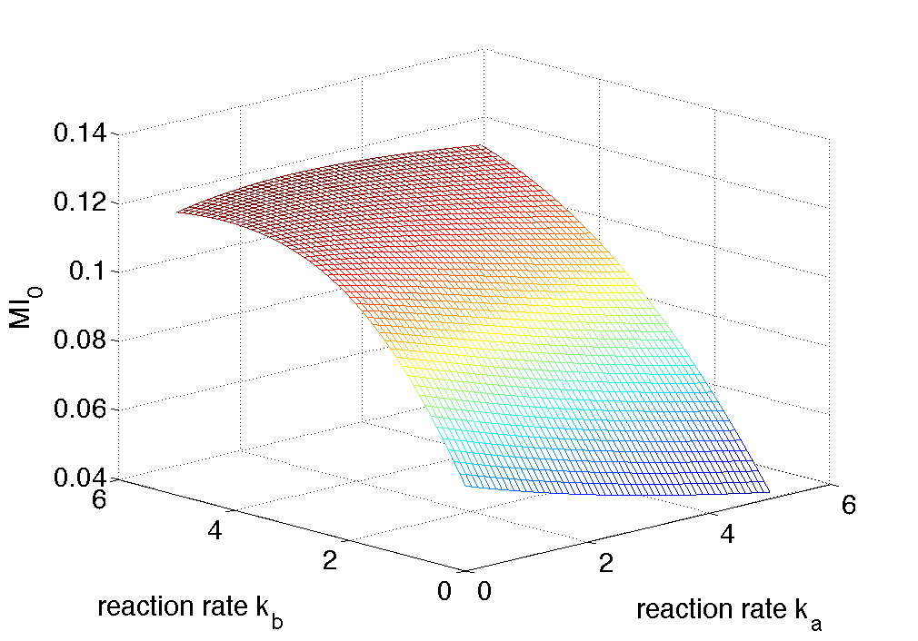
Figure 1. The change of $MI_{0}$ with varying $k_{a}$ and $k_{b}$.

References

- [1] L. Ambrosio, N. Gigli, and G. Savaré. Gradient flows: in metric spaces and in the space of probability measures. Springer, 2006.
- [2] D.F. Anderson. Stochastic perturbations of biochemical reaction systems. PhD thesis, Duke University, 2005.
- [3] D.F. Anderson. A proof of the global attractor conjecture in the single linkage class case. SIAM Journal on Applied Mathematics, 71(4):1487–1508, 2011.
- [4] D.F Anderson and A. Shiu. The dynamics of weakly reversible population processes near facets. SIAM Journal on Applied Mathematics, 70(6):1840–1858, 2010.
- [5] Rajendra B. A note on the lyapunov equation. Linear Algebra and its Applications, 259:71–76, 1997.
- [6] V.I. Bogachev, N.V. Krylov, and M. Röckner. On regularity of transition probabilities and invariant measures of singular diffusions under minimal conditions. Communications in Partial Differential Equations, 26(11-12):2037–2080, 2001.
- [7] E. Clark, A. Nellis, S. Hickinbotham, S. Stepney, T. Clarke, M. Pay, and P. Young. Degeneracy enriches artificial chemistry binding systems. In European Conference on Artificial Life, 2011.
- [8] M.V. Day and T.A. Darden. Some regularity results on the ventcel-freidlin quasi-potential function. Applied Mathematics and Optimization, 13(1):259–282, 1985.
- [9] C. Dellacherie and P. Meyer. Probabilities and potential, vol. 29 of north-holland mathematics studies, 1978.
- [10] G.M. Edelman and J.A. Gally. Degeneracy and complexity in biological systems. Proceedings of the National Academy of Sciences, 98(24):13763, 2001.
- [11] V. ery Roy. Noise perturbations of nonlinear dynamical systems. Chapter 6, in Computational Stochastic Mechanics, (A. H.-D. Cheng, and C. Y. Yang, Eds.), pages 125–148, 1993.
- [12] M. Feinberg. Lectures on chemical reaction networks. Notes of lectures given at the Mathematics Research Center, University of Wisconsin, 1979.
- [13] M. Feinberg. Chemical reaction network structure and the stability of complex isothermal reactors–i. the deficiency zero and deficiency one theorems. Chemical Engineering Science, 42(10):2229–2268, 1987.
- [14] M. Feinberg. The existence and uniqueness of steady states for a class of chemical reaction networks. Archive for Rational Mechanics and Analysis, 132(4):311–370, 1995.
- [15] A. Graham. Kronecker products and matrix calculus: With applications. JOHN WILEY & SONS, INC., 605 THIRD AVE., NEW YORK, NY 10158, 1982, 130, 1982.
- [16] KM Hargreaves and WM Pardridge. Neutral amino acid transport at the human blood-brain barrier. Journal of Biological Chemistry, 263(36):19392–19397, 1988.
- [17] W. Huang, M. Ji, Z. Liu, and Y. Yi. Concentration and limit behaviors of stationary measures. submitted, 2015.
- [18] Lars Jöres and Rolf Wagner. Essential steps in the ppgpp-dependent regulation of bacterial ribosomal rna promoters can be explained by substrate competition. Journal of Biological Chemistry, 278(19):16834–16843, 2003.
- [19] Yoosik Kim, María José Andreu, Bomyi Lim, Kwanghun Chung, Mark Terayama, Gerardo Jiménez, Celeste A Berg, Hang Lu, and Stanislav Y Shvartsman. Gene regulation by mapk substrate competition. Developmental cell, 20(6):880–887, 2011.
- [20] H. Kitano. Biological robustness. Nature Reviews Genetics, 5(11):826–837, 2004.
- [21] H. Kitano. Towards a theory of biological robustness. Molecular systems biology, 3(1), 2007.
- [22] S. Kullback. Information theory and statistics. Courier Dover Publications, 1997.
- [23] Y. Li, G. Dwivedi, W. Huang, M.L. Kemp, and Y. Yi. Quantification of degeneracy in biological systems for characterization of functional interactions between modules. Journal of Theoretical Biology, 302:29–38, 2012.
- [24] Y. Li and Y. Yi. Systematic measures of biological networks, part i: Invariant measures and entropy. Preprint, 2014.
- [25] D. Ludwig. Persistence of dynamical systems under random perturbations. Siam Review, pages 605–640, 1975.
- [26] Y.B. Pesin. Dimension theory in dynamical systems: contemporary views and applications. University of Chicago Press, 1997.
- [27] T Pocklington and J Jeffery. Competition of two substrates for a single enzyme. a simple kinetic theorem exemplified by a hydroxy steroid dehydrogenase reaction. Biochemical Journal, 112(3):331–334, 1969.
- [28] Sascha Schäuble, Anne Kristin Stavrum, Pål Puntervoll, Stefan Schuster, and Ines Heiland. Effect of substrate competition in kinetic models of metabolic networks. FEBS letters, 587(17):2818–2824, 2013.
- [29] J. Stelling, U. Sauer, Z. Szallasi, F.J. Doyle III, and J. Doyle. Robustness of cellular functions. Cell, 118(6):675–685, 2004.
- [30] G. Tononi, O. Sporns, and G.M. Edelman. Measures of degeneracy and redundancy in biological networks. Proceedings of the National Academy of Sciences of the United States of America, 96(6):3257, 1999.
- [31] J. Whitacre. Biological robustness: paradigms, mechanisms, and systems principles. Frontiers in genetics, 3:67, 2012.
- [32] J. Whitacre and S. Atamas. Degeneracy allows for both apparent homogeneity and diversification in populations. Biosystems, 110(1):34–42, 2012.
- [33] J. Whitacre and A. Bender. Degeneracy: a design principle for achieving robustness and evolvability. Journal of Theoretical Biology, 263(1):143–153, 2010.
- [34] R.W. Yeung. A first course in information theory, volume 1. Plenum Pub Corp, 2002.