Systematic Measures of Biological Networks, Part I: Invariant measures and Entropy

Abstract.

This paper is Part I of a two-part series devoting to the study of systematic measures in a complex biological network modeled by a system of ordinary differential equations. As the mathematical complement to our previous work [31] with collaborators, the series aims at establishing a mathematical foundation for characterizing three important systematic measures: degeneracy, complexity and robustness, in such a biological network and studying connections among them. To do so, we consider in Part I stationary measures of a Fokker-Planck equation generated from small white noise perturbations of a dissipative system of ordinary differential equations. Some estimations of concentration of stationary measures of the Fokker-Planck equation in the vicinity of the global attractor are presented. Relationship between differential entropy of stationary measures and dimension of the global attractor is also given.

1. Introduction

The concept of modular biology has been proposed and extensively investigated in the past several decades. In a complex biological network, modules in cells are created by interacting molecules that function in a semi-autonomous fashion and they are functionally correlated. To better understand the interactions between modules in a complex biological network, it is necessary to quantitatively study systematic properties such as degeneracy, robustness, complexity, redundancy, and evolvability.

Emerged from early studies of brain functions [14], notions of degeneracy and complexity were first introduced in neural networks in [45], and the robustness was studied in [30, 29] for systems with performance functions. Roughly speaking, in a cellular network or a neural network degeneracy measures the capacity of elements that are structurally different to perform the same function, structural complexity measures the magnitude of functional integration and local segregation of sub-systems, and the robustness measures the capacity of performing similar function under perturbation. These systematic measures are known to be closely related. Indeed, it has already been observed via numerical simulations for neural networks that high degeneracy not only yields high robustness, but also it is accompanied by an increase in structural complexity [46].

As increasing biological phenomena were being observed, quantitative studies of systematic measures in biological networks were also being conducted. For instance, numerical simulations revealed connections between degeneracy and complexity in artificial chemistry binding systems [7]; and also conclude that degeneracy underlies the presence of long range correlation in complex networks [11, 10]. Features like regulation and robustness of biochemical networks of signal transduction have also been studied quantitatively in [30, 42]. Degeneracy, complexity and robustness were quantified for neural networks by making use of testing noise injections into the networks in [46]. However, it was later remarked in the review article [13] that “degeneracy is a ubiquitous property of biological systems at all levels of organization, the concept has not yet been fully incorporated into biological thinking, $\dots$ because of the lack of a general evolutionary framework for the concept and the absence of a theoretical analysis”. Recently, quantification of degeneracy, complexity and robustness in biological networks modeled by systems of ordinary differential equations was made in the authors’ joint work [31] with Dwivedi, Huang and Kemp. The goal of that study is precisely to extend the concept of degeneracy to an evolutionary biological network and to establish its connections with complexity and robustness.

The present work, consisting of two parts, serves as the mathematical complement of our previous work [31], aiming at establishing a mathematical foundation of degeneracy, complexity and robustness in a complex biological network modeled by a system of ordinary differential equations.

This mathematical foundation is based on the theory of stochastic differential equations. In particular, considering testing white noise perturbations to a biological network is important in the quantification of its systematic measures because characterizations of degeneracy and complexity rely on the functional connections among modules of the network and such connections can be activated by injecting external noises, similarly to the case of neural systems [46, 31].

To be more precise, consider a biological network modeled by the following system of ordinary differential equations (ODE system for short):

(1.1) $$x^{\prime}=f(x),\;\;\;x\in{\mathbb{R}}^{n},$$

where $f$ is a $C^{1}$ vector field on ${\mathbb{R}}^{n}$, called drift field. Under additive white noise perturbations $\sigma dW_{t}$, we obtain the following system of stochastic differential equations (SDE system for short):

(1.2) $$\mathrm{d}X=f(X)\mathrm{d}t+\epsilon\sigma(x)\mathrm{d}W_{t},\;\;\;X\in{\mathbb{R}}^{n},$$

where $W_{t}$ is the standard $m$-dimensional Brownian motion, $\epsilon$ is a small parameter lying in an interval $(0,\epsilon^{*})$, and $\sigma$, called an noise matrix, is an $n\times m$ matrix-valued, bounded, $C^{1}$ function on ${\mathbb{R}}^{n}$ for some positive integer $m\geq n$, such that $\sigma(x)\sigma^{\top}(x)$ is everywhere positive definite in $\mathbb{R}^{n}$. We denote the collection of such noise matrices by $\Sigma$. Under certain dissipation condition (e.g., the existence of Lyapunov function corresponding to (1.2) assumed in this paper), the SDE system (1.2) generates a diffusion process in ${\mathbb{R}}^{n}$ which admits a transition probability kernel $P^{t}(x,\cdot)$, $t\geq 0$, $x\in{\mathbb{R}}^{n}$, such that for each $x\in\mathbb{R}^{n}$, $P^{t}(x,\cdot)$ is a probability measure and for each Borel set $B\subset\mathbb{R}^{n}$, $P^{t}(x,B)$ measures the probability of the stochastic orbit starting from $x$ entering the set $B$ at time $t$. An invariant probability measure of the diffusion process associated with (1.2) is the left invariant of $P^{t}(x,\cdot)$ such that

$$(\mu_{\epsilon}P^{t})(\cdot)=\int_{{\mathbb{R}}^{n}}P^{t}(x,\cdot)\mathrm{d}\mu_{\epsilon}=\mu_{\epsilon}(\cdot),\qquad t\geq 0\,.$$

An invariant probability measure associated with (1.2) is necessarily a stationary measure of the Fokker-Planck equation associated with (1.2). In general, a stationary measure can be regarded as a “generalized invariant measure” if the diffusion process fails to admit an invariant measure.

By injecting external fluctuation $\epsilon\sigma dW_{t}$ into the network (1.1), the connections among different modules of the network are activated. Assuming the existence of a stationary measure $\mu_{\epsilon}$ of the Fokker-Planck equation associated with (1.2) for each $\epsilon\in(0,\epsilon^{*})$, the mutual information among any two modules (coordinate subspaces) $X_{1},X_{2}$ can be defined using the margins $\mu_{1}$, $\mu_{2}$ of $\mu_{\epsilon}$ with respect to $X_{1},X_{2}$, respectively. Such mutual information can then be used to quantify degeneracy and complexity, and further to examine their connections with dynamical quantities like robustness.

Such a mathematical foundation for degeneracy, complexity, and robustness in a biological network relies on a quantitative understanding of the stationary measures $\mu_{\epsilon}$ particularly with respect to their concentrations. This is in fact the main subject of this part of the series.

A well-known approach to study the invariant probability measure is the classical large-deviation theory (or Freidlin-Wentzell theory). The probability that the trajectory of (1.2) stays in the neighborhood of any absolutely continuous function can be calculated explicitly by Girsanov’s theorem. This leads to some estimates of tails of stationary measures, or the first exit time of a stochastic orbit (see e.g. [12, 17, 28]). For instance, it is shown in [17] that for any set $P\subset\mathbb{R}^{n}$ that does not intersect with any attractor of (1.1), there exists a constant $V_{0}>0$ such that

(1.3) $$\lim_{\epsilon\rightarrow 0}\epsilon^{2}\log\mu_{\epsilon}(P)=-V_{0}.$$

In particular, the limit

(1.4) $$-\lim_{\epsilon\rightarrow 0}\epsilon^{2}\log\frac{\mathrm{d}\mu_{\epsilon}(x)}{\mathrm{d}x}:=V(x)\,,$$

if exists, is called the quasi-potential function.

One limitation of the large deviation theory is that usually it can only estimate the probability of rare events, which corresponds to the tails of stationary measures. In many applications, more refined analysis is based on the assumption that $\mu_{\epsilon}$ can be approximated by a Gibbs measure, i.e., $\mu_{\epsilon}$ admits a density function $u_{\epsilon}$ such that

(1.5) $$u_{\epsilon}(x)\approx\frac{1}{K}e^{-V(x)/\epsilon^{2}}\,,$$

where $V(x)$ is the quasi-potential function [41, 20, 44, 43]. However, this assumption is difficult to verify in general as it requires high regularity of the quasi-potential function. Rigorous results are only known for some simple systems [8, 9, 33].

To understand connections among degeneracy, complexity, and robustness, we need to measure the effects of stochastic perturbations in (1.2) at the same order as $\epsilon$. To make such estimation rigorously, we will adopt the level set method recently introduced in [26, 27] for stationary probability measures of the Fokker-Planck equation associated with (1.2) (see Section  2).

In this part of the series, we will mainly apply the level set method to obtain estimates on the concentrations of invariant measures $\mu_{\epsilon}$ with respect to a fixed $\sigma\in\Sigma$. Our main results of the paper lie in the following three categories.

1. Concentration in the vicinity of the global attractor $\mathcal{A}$: We will show in Theorem  3.3 that for any $0<\delta\ll 1$ there exists a constant $M>0$ such that

   $$\mu_{\epsilon}(\{x:\,\mathrm{dist}(x,\mathcal{A})\leq M\epsilon\})\geq 1-\delta.$$

   We will also show in Theorem  3.4 that for any $\alpha\in(0,1)$,

   $$\lim_{\epsilon\rightarrow 0}\mu_{\epsilon}(\{x:\,\epsilon^{1+\alpha}\leq\mathrm{dist}(x,\mathcal{A})\leq\epsilon^{1-\alpha}\})=1\,.$$

2. Mean square displacement: We will show in Theorem  3.5 under certain conditions that there exist constants $V_{1},V_{2}>0$ such that

   $$V_{1}\epsilon^{2}\leq V(\epsilon)\leq V_{2}\epsilon^{2},$$

   where

   $$V(\epsilon)=\int_{\mathbb{R}^{n}}\mathrm{dist}^{2}(x,\mathcal{A})d\mu_{\epsilon}(x).$$

3. Entropy-dimension relationship: We will show in Theorem  4.1 that if the global attractor $\mathcal{A}$ is regular, then

   $$\liminf_{\epsilon\rightarrow 0}\frac{\mathcal{H}(\mu_{\epsilon})}{\log\epsilon}\geq n-d$$

   where $\mathcal{H}(\mu_{\epsilon})$ is the differential entropy of $\mu_{\epsilon}$ and $d$ is the Minkowski dimension of $\mathcal{A}$.

The paper is organized as follows. Section  2 is a preliminary section in which we mainly review some results and the level set method from [26, 27, 25] on Fokker-Planck equations. Concentrations of stationary measures are studied in Section  3. We derive the entropy-dimension relationship in Section 4.

2. Preliminary

In this section, we will review some notions and known results about dissipative dynamical systems and Fokker-Planck equations including global attractors, Lyapunov functions, and the existence and uniqueness of stationary measures. We will also recall a Harnack inequality to be used later.

2.1. Dissipation and global attractor

We note that the system (1.1) generates a local flow on ${\mathbb{R}}^{n}$, which we denote by $\phi^{t}$. For $B\subset\mathbb{R}^{n}$, we denote $\phi^{t}(B)=\{\varphi^{t}(x)\ :\,\ x\in B\}$. A set $A\subset{\mathbb{R}}$ is said to be invariant with respect to (1.1) or $\varphi^{t}$ if $\varphi^{t}$ extends to a flow on $A$ and $\phi^{t}(A)\subset A$ for any $t\in{\mathbb{R}}$.

System (1.1) or $\phi^{t}$ is said to be dissipative if $\varphi^{t}$, $t\geq 0$, is a positive semi-flow on ${\mathbb{R}}^{n}$ and there exists a compact subset $K$ of ${\mathbb{R}}^{n}$ with the property that for any $\xi\in{\mathbb{R}}^{n}$ there exists a $t_{0}(\xi)>0$ such that $\varphi^{t}(\xi)\in K$ as $t\geq t_{0}(\xi)$. It is well-known that if $\varphi^{t}$ is dissipative, then it must admit a global attractor $\mathcal{A}$, i.e., $\mathcal{A}$ is a compact subset of $\mathbb{R}^{n}$ which attracts any bounded set in $\mathbb{R}^{n}$ in the sense that $\lim_{t\rightarrow+\infty}\mathrm{dist}(\varphi^{t}(K),\mathcal{A})=0$ for every bounded set $K\subset\mathbb{R}^{n}$, where $\mathrm{dist}(A,B)$ denote the Hausdorff semi-distance from a bounded set $A$ to a bounded set $B$ in $\mathbb{R}^{n}$. The global attractor $\mathcal{A}$ of $\varphi^{t}$, if exists, must be unique and invariant with respect to $\varphi^{t}$. In fact, $\varphi^{t}$ is dissipative if and only if it is a semi-flow admiting a global attractor. Moreover, dissipation of $\varphi^{t}$ can be guaranteed by the existence of a Lyapunov function $U$ of (1.1), i.e., $U\in C^{1}({\mathbb{R}}^{n})$ is a non-negative function such that $U(x)<\sup_{x\in{\mathbb{R}}^{n}}U(x)$, $x\in{\mathbb{R}}^{n}$, and there exist a compact set $K\subset{\mathbb{R}}^{n}$ and a constant $\gamma>0$, called a Lyapunov constant, such that

$$f(x)\cdot\nabla U(x)\leq-\gamma,\;\qquad x\in{\mathbb{R}}^{n}\setminus K.$$

The global attractor $\mathcal{A}$ of (1.1) is said to be a strong attractor if there is a connected open neighborhood $\mathcal{N}$ of $\mathcal{A}$ with $C^{2}$ boundary, called isolating neighborhood, such that i) $\omega(\mathcal{N})=\mathcal{A}$ and ii) $f(x)\cdot\nu(x)<0$ for each $x\in\partial\mathcal{N}$, where $\nu(x)$ is the outward normal vector of $\mathcal{N}$ at $x$ and $\omega(B):=\bigcap_{\tau\geq 0}\overline{\{\varphi^{t}(B)\ :\,\ t\geq\tau\}}$ is the $\omega$-limit set of a bounded set $B\subset\mathbb{R}^{n}$. It is clear that $\mathcal{A}$ is a strong attractor of (1.1) if there exists a strong Lyapunov function in a connected open set $S\subseteq{\mathbb{R}}^{n}$ containing $\mathcal{A}$, i.e., $\nabla U(x)\neq 0$, $x\in S\setminus\mathcal{A}$, and there is a constant $\gamma_{0}>0$ such that

$$f(x)\cdot\nabla U(x)\leq-\gamma_{0}|\nabla U(x)|^{2},\;\qquad x\in S\setminus\mathcal{A}.$$

We again refer the constant $\gamma_{0}$ above to as the Lyapunov constant of $U$.

2.2. Fokker-Planck equation and stationary measures

If the transition probability kernel $P^{t}(x,\cdot)$ of the SDE system (1.2) admits a probability density function $p^{t}(x,z)$, i.e.,

$$P^{t}(x,B)=\int_{B}p^{t}(x,z)\mathrm{d}z$$

for any Borel set $B\subset\mathbb{R}^{n}$, then for any measurable, non-negative function $\xi(x)$ with $\int_{\mathbb{R}^{n}}\xi(x)\mathrm{d}x=1$, $u_{\epsilon}(x,t)=\int_{\mathbb{R}^{n}}p^{t}(z,x)\xi(z)\mathrm{d}z$ characterizes the time evolution of the probability density function. Formally, $u_{\epsilon}(x,t)$ satisfies the following Fokker-Planck equation (FPE for short) :

(2.1) $$\left\{\begin{array}[]{l}\displaystyle{\frac{\partial u_{\epsilon}(x,t)}{\partial t}=\frac{1}{2}{{\epsilon}^{2}}\sum\limits_{i,j=1}^{n}{\partial_{ij}(a_{ij}(x)u_{\epsilon}(x,t))-\sum_{i=1}^{n}\partial_{i}(f(x)u_{\epsilon}(x,t))}:=L_{\epsilon}u_{\epsilon}(x,t),}\\ \displaystyle{\int_{{\mathbb{R}}^{n}}u_{\epsilon}(x,t)\rm dx=1},\end{array}\right.$$

where $(a_{ij}(x)):=A(x):=\sigma(x){{\sigma}^{\top}}(x)$ is an $n\times n$, everywhere positive definite, matrix-valued $C^{1}$ function, called diffusion matrix. The operator $L_{\epsilon}$ is called Fokker-Planck operator.

Among solutions of the Fokker-Planck equation, of particular importance are the stationary solutions. For any connected open subset $S\subset\mathbb{R}^{n}$, stationary solutions on $S$ satisfy the stationary Fokker-Planck equation

(2.2) $$L_{\epsilon}u_{\epsilon}(x,t)=0\,,\quad\int_{S}u_{\epsilon}(x,t)\mathrm{d}x=1\,,\qquad u\geq 0\,.$$

More generally, on any connected open subset $S\subset\mathbb{R}^{n}$, a stationary measure of the Fokker-Planck equation is a probability measure $\mu_{\epsilon}$ satisfying

$$\int_{S}\mathcal{L}_{\epsilon}h(x)\mathrm{d}\mu_{\epsilon}=0\,,\quad\forall h(x)\in C_{0}^{\infty}(S)\,,$$

where

$$\mathcal{L}_{\epsilon}=\frac{1}{2}\epsilon^{2}\sum_{i,j=1}^{n}a_{ij}(x)\partial_{ij}+\sum_{i=1}^{n}f_{i}(x)\partial_{i}$$

is the adjoint Fokker-Planck operator.

If $u_{\epsilon}$ is a stationary solution of the Fokker-Planck equation (2.1), then $u_{\epsilon}{\rm d}x$ is clearly a stationary measure. Conversely, it follows from the regularity theory of Fokker-Planck equation [3] and standard regularity theory of elliptic equation that a stationary measure of Fokker-Planck equation (2.1) must admit a density function which is a strictly positive, classical stationary solution of the Fokker-Planck equation. Note that a classical solution means a solution that has enough regularity to be plugged into the original differential equation.

An invariant measure of the diffusion process generated by (1.2), or equivalently, of the transition probability kernel $P^{t}$, is necessarily a stationary measure of the corresponding Fokker-Planck equation (2.1). The converse needs not be true in general. However, stationary measures considered in this paper are in fact invariant measures of the diffusion process generated by (1.2).

The existence and estimates of stationary measures of (2.1) are related to Lyapunov-like functions associated with it. For the sake of generality, we consider a connected open set $S\subseteq\mathbb{R}^{n}$. A non-negative function $U\in C(S)$ is said to be a compact function if (i) $U(x)<\rho_{M}$, $x\in S$; and (ii) $\lim_{x\rightarrow\partial S}U(x)=\rho_{M}$, where $\rho_{M}=\sup_{x\in S}U(x)$ is called the essential upper bound of $U$. In the case $S={\mathbb{R}}^{n}$, $x\rightarrow\partial S$ simply means that $x\to\infty$. It is obvious that Lyapunov and strong Lyapunov functions defined in the previous subsection are all compact functions on ${\mathbb{R}}^{n}$.

For a compact function defined on $S$ and for each $\rho\in[0,\rho_{M})$, we denote $\Omega_{\rho}(U)=\{x\in S:U(x)<\rho\}$ as the $\rho$-sublevel set of $U$ and $\Gamma_{\rho}(U)=\{x\in S:U(x)=\rho\}$ as the $\rho$-level set of $U$.

Let $U$ be a compact $C^{2}$ function on a connected open set $S\subset\mathbb{R}^{n}$ with upper bound $\rho_{M}$. For a fixed $\epsilon\in(0,\epsilon^{*})$, $U$ is called a Lyapunov function associated with (2.1) (on $S$) if there are constants $\rho_{m},\gamma>0$, referred to as an essential lower bound, the Lyapunov constant of $U$, respectively, such that

$$\mathcal{L}_{\epsilon}U(x)<-\gamma,\;\qquad x\in S\setminus\Omega_{\rho_{m}}(U).$$

$U$ is called a weak Lyapunov function (on $S$) associated with equation (2.1) if there is a constant $\rho_{m}$, still referred to as an essential lower bound of $U$, such that

$$\mathcal{L}_{\epsilon}U(x)\leq 0,\;\qquad x\in S\setminus\Omega_{\rho_{m}}(U)\,.$$

If $U(x)$ is a Lyapunov function (resp. weak Lyapunov function ) associated with (2.1) for each $\epsilon\in(0,\epsilon^{*})$ and the essential lower bound and Lyapunov constant are independent of $\epsilon$, then $U(x)$ is called a uniform Lyapunov function (resp. uniform weak Lyapunov function) associated with the family (2.1) on $(0,\epsilon^{*})$.

It is easy to see that a uniform Lyapunov function associated with the family (2.1) on $(0,\epsilon^{*})$ must be a Lyapunov function for the ODE system (1.1). Consequently, if the family (2.1) on $(0,\epsilon^{*})$ admits a uniform Lyapunov function, then the ODE system (1.1) must be dissipative and hence admits a global attractor.

There has been extensive studies on the existence and uniqueness of stationary measures of Fokker-Planck equation (2.1) (see [4, 5, 27] and references therein). While stationary measures of a Fokker-Planck equation in a bounded domain of ${\mathbb{R}}^{n}$ always exist, the existence of such in the entire space (i.e. $S=\mathbb{R}^{n}$) necessarily require certain dissipation conditions at infinity which is more or less equivalent to the existence of a Lyapunov function.

The following theorem follows from the main result of [5, 27] and the standard regularity theory of elliptic equations.

Theorem 2.1.

If the family ${\mathcal{L}}_{\epsilon}$, $\epsilon\in(0,\epsilon^{*})$, admits an unbounded uniform Lyapunov function, then for each $\epsilon\in(0,\epsilon^{*})$, the corresponding Fokker-Planck equation (2.1) has a unique stationary measure $\mu_{\epsilon}$ on $\mathbb{R}^{n}$. Moreover, ${\rm d}\mu_{\epsilon}(x)=u_{\epsilon}(x){\rm d}x$ for a classical stationary solution $u_{\epsilon}$ of (2.1).

2.3. Level set method and measure estimates

The following two theorems are the main ingredient of the level set method introduced in [26].

Theorem 2.2.

(Integral identity, Theorem 2.1, [26]) For a given $\epsilon\in(0,\epsilon^{*})$, let $u=u_{\epsilon}$ be a stationary solution of (2.1). Then for any Lipschitz domain $S\subset{\mathbb{R}}^{n}$ and a function $F\in C^{2}(S)$ having constant value on $\partial S$,

$$\int_{S}({\mathcal{L}}_{\epsilon}F(x))u(x)\mathrm{d}x = \int_{S}\left(\sum_{i,j=1}^{n}\frac{1}{2}\epsilon^{2}a_{ij}(x)\partial^{2}_{ij}F(x)+\sum_{i=1}^{n}f_{i}(x)\partial_{i}F(x)\right)u(x)\mathrm{d}x$$

$$= \int_{\partial S}\left(\sum_{i=1}^{n}\sum_{j=1}^{n}\frac{1}{2}\epsilon^{2}a_{ij}(x)\partial_{i}F(x)\nu_{j}\right)u(x)\mathrm{d}s$$

where $\{\nu_{j}\}_{j=1}^{n}$ denotes the unit outward normal vectors.

In applying Theorem  2.2 to study stationary solutions of a Fokker-Planck equation, one typically considers $F$ as a Lyapunov function $U(x)$ and $S$ as a sublevel set $\Omega_{\rho}(U)=\{x\in{\mathbb{R}}^{n}:U(x)<\rho\}$. When $\nabla U(x)\neq 0$ on the level set $\Gamma_{\rho}(U)=\{x\in{\mathbb{R}}^{n}:U(x)=\rho\}$, we note that $\partial\Omega_{\rho}(U)=\Gamma_{\rho}(U)$.

Theorem 2.3.

(Derivative formula, Theorem 2.2, [26]) Let $\mu$ be a Borel probability measure with density function $u\in C({\mathbb{R}}^{n})$ and $U$ be a $C^{1}$ compact function on ${\mathbb{R}}^{n}$ such that $\nabla U(x)\neq 0$, $x\in\Gamma_{\rho}(U)$ for all $\rho$ lying in an interval $(\rho_{1},\rho_{2})$. Then

$$\frac{\partial}{\partial\rho}\int_{\Omega_{\rho}(U)}u(x)~{}{\rm d}x=\int_{\Gamma_{\rho}(U)}\frac{u(x)}{|\nabla U(x)|}~{}{\rm d}s,\qquad\rho\in(\rho_{1},\rho_{2}).$$

Let $\mu_{\epsilon}$ be a stationary measures of the Fokker-Planck equation (2.1). Then as shown in [26, 27], Theorems  2.2, 2.3 yield the following estimates concerning $\mu_{\epsilon}$ in the presence of a Lyapunov function.

Lemma 2.1.

(Theorem A (b), [26]) Assume that (2.1) admits a Lyapunov function $U$ with essential lower, upper bound $\rho_{m}$, $\rho_{M}$, respectively, that satisfies $\nabla U(x)\neq 0$, $x\in\Gamma_{\rho}$ for almost every $\rho\in[\rho_{m},\rho_{M})$. Then for any function $H(\rho)\in L^{1}_{loc}([\rho_{m},\rho_{M}))$ with

$$H(\rho)\geq\frac{1}{2}\epsilon^{2}\sum_{i,j=1}^{n}a_{ij}(x)\partial_{x_{i}}U(x)\partial_{x_{j}}U(x),\quad x\in\Gamma_{\rho},$$

one has

$$\mu_{\epsilon}(\Omega_{\rho_{M}}(U)\setminus\Omega_{\rho}(U))\leq e^{-\gamma\int_{\rho_{m}}^{\rho}\frac{1}{H(t)}dt},\qquad\rho\in[\rho_{m},\rho_{M}),$$

where $\gamma>0$ is the Lyapunov constant of $U$.

Lemma 2.2.

(Theorem A (c), [26]) Assume that (2.1) admits a weak Lyapunov function $U$ in a connected open set $S\subseteq\mathbb{R}^{n}$ with essential lower, upper bound $\rho_{m},\rho_{M}$, respectively. Also assume that $(a_{ij})$ is everywhere positive definite in $S$. Then for any two positive continuous functions $H_{1}(\rho),H_{2}(\rho)$ satisfying

$$H_{1}(\rho)\leq\frac{1}{2}\epsilon^{2}\sum_{i,j=1}^{n}a_{ij}(x)\partial_{i}U(x)\partial_{j}U(x)\leq H_{2}(\rho),\quad x\in\Gamma_{\rho}(U),$$

one has

$$\mu_{\epsilon}(\Omega_{\rho_{M}}(U)\setminus\Omega_{\rho_{m}}(U))\leq\mu_{\epsilon}(\Omega_{\rho}(U)\setminus\Omega_{\rho_{m}}(U))e^{\int_{\rho}^{\rho_{M}}\frac{1}{\tilde{H}(s)}\mathrm{d}s},\qquad\;\rho\in(\rho_{m},\rho_{M}),$$

where $\tilde{H}(\rho)=H_{1}(\rho)\int_{\rho_{m}}^{\rho}H^{-1}_{2}(s)\mathrm{d}s$.

2.4. Hanack inequality

We recall the following Harnack inequality from [18].

Lemma 2.3.

Consider an elliptic operator

$$Lu(x)=\sum_{i,j=1}^{n}\partial_{i}(a_{ij}(x)\partial_{j}u(x))+\sum_{i=1}^{n}\partial_{i}(b_{i}(x)u(x))+\sum_{i=1}^{n}c_{i}(x)\partial_{i}u(x)+d(x)u(x)$$

in a domain $\Omega\subset\mathbb{R}^{n}$. Let $\lambda$ and $\Lambda$ be two constants depend on matrix $\{a_{ij}(x)\}$ such that

$$\sum_{i,j=1}^{n}a_{ij}(x)\zeta_{i}\zeta_{j}\geq\lambda|\zeta|^{2}$$

and

$$\sum_{i,j=1}^{n}|a_{ij}(x)|^{2}\leq\Lambda^{2}\,.$$

Let $\nu$ be a constant such that

$$\lambda^{-2}\sum_{i=1}^{n}(|b_{i}(x)|^{2}+|c_{i}(x)|^{2}+\lambda^{-1}|d(x)|)\leq\nu^{2}\,.$$

Then for any ball $B_{4R}(y)\subset\Omega$, we have

$$\sup_{x\in B_{R}(y)}u(x)\leq C\inf_{x\in B_{R}(y)}u(x)$$

where $C\leq C_{0}(n)^{(\Lambda/\lambda+\nu R)}$.

3. Concentration of stationary measures

We make the following standard hypothesis:

• System (1.1) is dissipative and there exists a strong Lyapunov function $W(x)$ with respect to an isolating neighborhood $S:=\mathcal{N}$ of the global attractor $\mathcal{A}$ such that

  $$W(x)\geq L_{1}\mathrm{dist}^{2}(x,\mathcal{A}),\;\;x\in\mathcal{N}$$

  for some $L_{1}>0$.

Remark 3.1.

When $\mathcal{A}$ is an equilibrium or a limit cycle, the stable foliation theorem asserts that a neighborhood $\mathcal{N}$ of $\mathcal{A}$ can be taken as a ball, and consequently $W(x)$ can be taken as $\mathrm{dist}(x,\mathcal{A})^{2}$.

When noises are added to the ODE system (1.1), our theory requires characterizations and estimates of stochastic quantities such as mean square displacement and entropy-dimension formula of stationary measures of the Fokker-Planck equation (2.1) associated with the SDE system (1.2). It turns out that, for these quantities to be well-defined, the following condition on the stationary measures of (2.1) is needed:

• For each $\epsilon\in(0,\epsilon^{*})$, the Fokker-Planck equation (2.1) admits a unique stationary measure $\mu_{\epsilon}$ such that

  $$\lim_{\epsilon\rightarrow 0}\frac{\mu_{\epsilon}(\mathbb{R}^{n}\setminus\mathcal{N})}{\epsilon^{2}}=0,$$

  and moreover, there are constants $p,R_{0}>0$ such that

  $$\mu_{\epsilon}(\{x\,:\,|x|>r\})\leq e^{-\frac{r^{p}}{\epsilon^{2}}}$$

  for all $r>R_{0}$ and all $\epsilon\in(0,\epsilon^{*})$.

Throughout the rest of the paper, for any fixed $\epsilon\in(0,\epsilon^{*})$, we let $\mu_{\epsilon}$ denote the unique stationary probability measure of (1.2) or the stationary measure of (2.1) and let $u_{\epsilon}(x)$ or, when it does not cause confusion, $u(x)$ stand for the (classical) stationary solution of equation (2.2), which is the density function of $\mu_{\epsilon}$.

To estimate these stochastic quantities mentioned above rigorously, it is essential to perform estimates on the concentration of $\mu_{\epsilon}$ both near and away from $\mathcal{A}$. In Section 3.1, we will conduct estimates on the local concentration of $\mu_{\epsilon}$ in the vicinity of $\mathcal{A}$ by making use of assumption H⁰) and give estimates of the tails of $\mu_{\epsilon}$ by providing a sufficient condition which ensures the validity of the condition H¹).

We remark that the estimation in Section 3.1 only provides one of many approaches to verify H⁰) and H¹). Essentially H¹) assumes that $\mu_{\epsilon}$ has sufficient concentration on an isolating neighborhood such that we can focus on the local analysis in the vicinity of the global attractor. As discussed in Example 3.2 below, such concentration is satisfied by many problems in applications, although it may be difficult to give generic sufficient conditions. In particular, the quasi-potential function defined in (1.4), if exists, leads to the desired concentration of $\mu_{\epsilon}$ immediately. If a quasi-potential function as in (1.4) exists and is differentiable, then it is a Lyapunov function of (1.1) [17]. This provides an alternative way of verifying H⁰). For results regarding high regularity of the quasi-potential function, see [8, 9].

3.1. Estimating tails of stationary measures

The purpose of this subsection is to provide an alternative way to verify assumption H⁰) and H¹). This is important in applications as rigorously verifying the quasi-potential landscape may be difficult for some models. Instead of using the quasi-potential function, we use a suitable Lyapunov function of system (1.1) to facilitate our study. To characterize the property of the desired Lyapunov function, the following definitions are necessary.

A compact function $U$ on a connected open set $S\subset{\mathbb{R}}^{n}$ is said to be of the class $\mathcal{B}^{*}$ in $S$ if there is a constant $p>0$ and a function $H(\rho)\in L^{1}_{loc}([\rho_{0},\rho_{M}))$ such that

$$H(\rho)\geq|\nabla U(x)|^{2},\quad x\in\Gamma_{\rho}(U)$$

and

$$\int_{\rho_{0}}^{\rho}\frac{1}{H(s)}\mathrm{d}s\geq|x|^{p},\quad x\in\Gamma_{\rho}(U)$$

for all $\rho\in(\rho_{0},\rho_{M})$, where $\rho_{0}=\inf_{x\in S}(x)$.

Remark 3.2.

According to the definition, a compact function $U(x)$ is of class $\mathcal{B}^{*}$ in $\mathbb{R}^{n}$ if (i) $U(x)$ has bounded first order derivative and (ii) $\lim_{|x|\rightarrow\infty}\frac{U(x)}{|x|^{p}}>0$ for some $p>0$. We will show that when (2.1) admits a class $\mathcal{B}^{*}$ Lyapunov function, its stationary measure has an exponential tail. One example of class $\mathcal{B}^{*}$ function will be given at the end of this subsection.

We will estimate the tails of stationary measures of (2.1) by dividing ${\mathbb{R}}^{n}\setminus\mathcal{N}$ into two regions: a neighborhood ${\mathcal{N}}_{\infty}$ of $\infty$ in ${\mathbb{R}}^{n}$, i.e., the complement of a sufficiently large compact set, and the intermediate region ${\mathcal{N}}_{*}$ between ${\mathcal{N}}_{\infty}$ and $\mathcal{N}$. We make the following hypothesis:

• There is a positive function $U\in C^{2}({\mathbb{R}}^{n}\setminus\mathcal{A})$ satisfying the following properties:

  • $\lim_{x\to\infty}U(x)=\infty$;

  • There exists a constant $\rho_{m}>0$ such that $U$ is a uniform Lyapunov function of the family (2.1) of class ${\mathcal{B}}^{*}$ in ${\mathcal{N}}_{\infty}=:\mathbb{R}^{n}\setminus\Omega_{\rho_{m}}(U)$;

  • There exists a constant $\bar{\rho}_{m}\in(0,\rho_{m})$ such that $U$ is a uniform weak Lyapunov function of the family (2.1) in ${\mathcal{N}}_{*}=:{\mathbb{R}}^{n}\setminus{\mathcal{N}}_{\infty}\setminus\Omega_{\bar{\rho}_{m}}(U)=\Omega_{\rho_{m}}(U)\setminus\Omega_{\bar{\rho}_{m}}(U)$;

  • $\nabla U(x)\neq 0$, $x\in{\mathbb{R}}^{n}\setminus\Omega_{\bar{\rho}_{m}}(U)$;

  • $\Omega_{\bar{\rho}_{m}}(U)\subset{\mathcal{N}}$.

Remark 3.3.

1) We note that when H²) holds, Theorem  2.1 asserts the existence of a unique stationary measure of (2.1) for each $\epsilon\in(0,\epsilon_{*})$.

2) With the hypotheses H⁰), H²), the ODE system (1.1) is dissipative in ${\mathcal{N}}_{\infty}$, strongly dissipative in $\mathcal{N}$, and remains dissipative in ${\mathcal{N}}_{*}$ but with small dissipation rate proportional to $\epsilon^{2}$.

3) The purpose of introducing H²) is to give a Lyapunov function-based sufficient condition of H⁰) and H¹). Except in this subsection, our estimates are based only on H⁰) and H¹).

We first estimate the concentration of stationary measures of (2.1) in the region ${\mathcal{N}}_{\infty}$, which verifies the second part of H¹).

Proposition 3.1.

If H²) holds, then there exist positive constants $\beta,R_{0},p$ such that

$$\mu_{\epsilon}(\mathbb{R}^{n}\setminus B(0,r))\leq e^{-\beta\frac{r^{p}}{\epsilon^{2}}},\qquad\epsilon\in(0,\epsilon_{*})\,,$$

for all $r\geq R_{0}$.

Proof.

Let $U$ be the uniform Lyapunov function of (2.1) for $\epsilon\in(0,\epsilon_{*})$, according to H²). Since $U$ is of class ${\mathcal{B}}^{*}$ in ${\mathcal{N}}_{\infty}$, there is a function $H(\rho)\in L^{1}_{loc}([\rho_{m},\infty))$, where $\rho_{m}$ denotes the essential lower bound of $U$, such that

$$H(\rho)\geq|\nabla U(x)|^{2},\quad x\in\Gamma_{\rho}(U)$$

and

$$\int_{\rho_{m}}^{\rho}\frac{1}{H(s)}\mathrm{d}s\geq|x|^{p},\quad x\in\Gamma_{\rho}(U)$$

for all $\rho>\rho_{m}$. Using positive definiteness of $A(x)$, we let $C_{0}>0$ be a constant such that

$$\epsilon^{2}H(\rho)\geq C_{0}\frac{1}{2}\epsilon^{2}\sum_{i,j=1}^{n}a_{ij}\partial_{i}U(x)\partial_{j}U(x)$$

and denote $H_{1}(\rho)=\epsilon^{2}H(\rho)/C_{0}$. It follows from Lemma  2.1 that

$$\mu_{\epsilon}(\mathbb{R}^{n}\setminus\Omega_{\rho}(U))\leq e^{-\gamma\int_{\rho_{m}}^{\rho}\frac{1}{H_{1}(s)}\mathrm{d}s}\leq e^{-\frac{\gamma C_{0}}{\epsilon^{2}}\int_{\rho_{m}}^{\rho}\frac{1}{H(s)}\mathrm{d}s}\leq e^{-\frac{\gamma C_{0}}{\epsilon^{2}}|x|^{p}}$$

for each $x\in\Gamma_{\rho}(U)$ whenever $\rho>\rho_{m}$, where $\gamma>0$ is the Lyapunov constant of $U$.

Let $R_{0}=\max_{x\in\Gamma_{r_{m}}(U)}|x|$, and for each $r\geq R_{0}$, denote $\rho(r)=\min_{|y|=r}U(y)$. Let $r\geq R_{0}$ and take $x\in\Omega_{\rho(r)}\cap B(0,r)$. Then $\Omega_{\rho(r)}\subset B(0,r)$ and

$$\mu_{\epsilon}(\mathbb{R}^{n}\setminus B(0,r))\leq\mu_{\epsilon}(\mathbb{R}^{n}\setminus\Omega_{\rho(r)}(U))\leq e^{-\frac{\gamma C_{0}}{\epsilon^{2}}|x|^{p}}=e^{-\frac{\beta}{\epsilon^{2}}r^{p}},$$

where $\beta=\tau C_{0}$. ∎

Next, we estimate the concentration of stationary probability measures of (2.1) in the intermediate region ${\mathcal{N}}_{*}$ to verify the first part of H¹) . For any connected open set $S\subset{\mathbb{R}}^{n}$, we note that $\mu_{\epsilon}|_{S}=:\mu_{\epsilon}/\mu_{\epsilon}(S)$ is a stationary probability measure of (2.1) on $S$.

Lemma 3.1.

Assume H⁰) and let $W$ be as in H⁰) and $\rho_{0}>0$ be such that $\Omega_{\rho_{0}}(W)\subset\mathcal{N}$ and $\Gamma_{\rho_{0}}\cap\mathcal{A}\neq\emptyset$. Then there is an $\epsilon_{0}\in(0,\epsilon_{*})$ such that

$$\mu_{\epsilon}(\mathcal{N}\setminus\Omega_{\rho_{0}}(W))\leq e^{-\frac{C_{1}}{\epsilon^{2}}},\qquad\epsilon\in(0,\epsilon_{0}),$$

where $C_{1}>0$ is a constant independent of $\epsilon$.

Proof.

It is easy to see that there exists an $\epsilon_{0}\in(0,\epsilon_{*})$ such that $W$ becomes a uniform Lyapunov function of (2.1) for all $\epsilon\in(0,\epsilon_{0})$ in $S=:\mathcal{N}$, with upper bound $\rho^{0}=\sup\{\rho>0:\Omega_{\rho}(W)\subset\mathcal{N}\}$ and essential lower bound $\rho_{0}$. The lemma now follows from an application of Lemma  2.1 to $\mu_{\epsilon}|_{\mathcal{N}}$ with

$$H(\rho)=\frac{1}{2}\epsilon^{2}\min_{x\in\Gamma_{\rho}(W)}(\sum_{i,j=1}^{n}a_{ij}(x)\partial_{x_{i}}W(x)\partial_{x_{j}}W(x)),\qquad\rho\in(\rho_{0},\rho^{0}).$$

∎

Proposition 3.2.

Assume H⁰), H²) and let $W$ be as in H⁰) and $R_{0}$ be as in Proposition 3.1. Then there are constants $\rho_{0},c_{0}>0$ and $\epsilon_{0}\in(0,\epsilon_{*})$ such that

$$\mu_{\epsilon}(B(0,R_{0})\setminus\Omega_{\rho_{0}}(W))\leq e^{-\frac{c_{0}}{\epsilon^{2}}},\qquad\epsilon\in(0,\epsilon_{0})\,.$$

Proof.

Let $U,\rho_{m},\bar{\rho}_{m}$ be as in H²) and $\bar{\rho}_{M}\in(\rho_{m},\infty)$ be such that $B(0,R_{0})\subset\Omega_{\bar{\rho}_{M}}(U)$. Without loss of generality, we assume that $\Gamma_{\bar{\rho}_{m}}(U)\cap\mathcal{A}=\emptyset$. Denote $\rho^{0}=\sup\{\rho>0:\Omega_{\rho}(W)\subset\mathcal{N}\}$ and let $\rho_{0}\in(0,\rho^{0})$, $\bar{\rho}_{*}\in(\rho_{0},\rho^{0})$ be such that $\Gamma_{\bar{\rho}_{0}}(W)\cap\mathcal{A}=\emptyset$, $\Omega_{\rho_{0}}(W)\subset\Omega_{\bar{\rho}_{m}}(U)\subset\Omega_{\bar{\rho}_{*}}(U)\subset\Omega_{\rho^{0}}(W)$.

By Lemma 3.1, there exists an $\epsilon_{0}>0$ and a constant $C_{1}>0$ such that

(3.1) $$\mu_{\epsilon}(\mathcal{N}\setminus\Omega_{\rho_{0}}(W))\leq e^{-\frac{C_{1}}{\epsilon^{2}}},\qquad\epsilon\in(0,\epsilon_{0}).$$

Since $U$ is a uniform Lyapunov function of (2.1) for $\epsilon\in(0,\epsilon_{*})$ on $S=:\Omega_{\bar{\rho}_{M}}(U)$, an application of Lemma 2.2 to $\mu_{\epsilon}|_{S}$ with

$$H_{1}(\rho)=\frac{1}{2}\epsilon^{2}\min_{x\in\Gamma_{\rho}(U)}(\sum_{i,j=1}^{n}a_{ij}(x)\partial_{i}U(x)\partial_{j}U(x)),$$

$$H_{2}(\rho)=\frac{1}{2}\epsilon^{2}\max_{x\in\Gamma_{\rho}(U)}(\sum_{i,j=1}^{n}a_{ij}(x)\partial_{i}U(x)\partial_{j}U(x)),\quad\rho\in(\bar{\rho}_{m},\bar{\rho}_{M}),$$

yields that there is a constant $C_{2}>0$ independent of $\epsilon$ such that

(3.2) $$\mu_{\epsilon}(B(0,R_{0})\setminus\Omega_{\rho_{0}}(W)) \leq \mu_{\epsilon}(S\setminus\Omega_{\bar{\rho}_{m}}(U))+\mu_{\epsilon}(\mathcal{N}\setminus\Omega_{\rho_{0}}(W))$$

$$\leq C_{2}\mu_{\epsilon}(\Omega_{\bar{\rho}_{*}}(U)\setminus\Omega_{\bar{\rho}_{m}}(U))+\mu_{\epsilon}(\mathcal{N}\setminus\Omega_{\rho_{0}}(W))$$

$$\leq (C_{2}+1)\mu_{\epsilon}(\mathcal{N}\setminus\Omega_{\rho_{0}}(W)).$$

The proposition now easily follows from (3.1), (3.2).

∎

Now, Propositions 3.1, 3.2 immediately yields the following result.

Corollary 3.1.

Conditions H⁰), H²) imply H¹).

Below, we give a simple example that satisfies H⁰) and H²).

Example 3.1.

Consider

(3.3) $$\left\{\begin{array}[]{l}x^{\prime}=y+x(1-x^{2}-y^{2})\\ y^{\prime}=-x+y(1-x^{2}-y^{2}).\end{array}\right.$$

Let

$$U(x,y)=\sqrt{x^{2}+y^{2}}h(\sqrt{x^{2}+y^{2}})+(x^{2}+y^{2}-1)^{2}(1-h(\sqrt{x^{2}+y^{2}}))$$

where $h(r)$ is a nonnegative nondecreasing $C^{2}$ cut-off function such that $h(r)=0$ for $r\leq 1.3$ and $h(r)=1$ for $r\geq 1.4$. Then it is easy to verify that $U(x,y)$ is of class $\mathcal{B}^{*}$ in $\{(x,y)\,:\,\sqrt{x^{2}+y^{2}}\geq 1.4\}$. When $\epsilon$ is sufficiently small, the other conditions in H²) and H⁰) are also satisfied.

Remark 3.4.

Example 3.1 is not a biological example. The purpose of having this simple example is to show that two Lyapunov functions can be “glued” to verify H²). In applications, if an ODE system has inward-pointing vector field far away from the origin, it is usually easy to find a Lyapunov function of class $\mathcal{B}^{*}$ in $\mathcal{N}_{\infty}$. This Lyapunov function in $\mathcal{N}_{\infty}$ may not have the Lyapunov property near the attractor. On the other hand, many ODE systems in biological models, such as mass-action systems, admit natural Lyapunov functions [23, 19, 15, 16], which are not of class $\mathcal{B}^{*}$ in $\mathcal{N}_{\infty}$. Often two Lyapunov functions can be “glued” together to satisfy H²), which, by Corollary 3.1, rigorously leads to the desired concentration of $\mu_{\epsilon}$ needed in the rest of this paper. We remind readers that there are some systematic ways to propagate “local” Lyapunov functions to construct a global Lyapunov function [2, 21], which can be used to check the validity of H²) in applications.

Example 3.2 (Toggle switch model).

Consider a gene circuit that consists of two genes $G_{A}$ and $G_{B}$. $G_{A}$ and $G_{B}$ produces proteins $A$ and $B$, respectively. Assume that protein $A$ can turn off gene $G_{B}$ by binding with its promotor, and vice versa. Once turned off, each gene turns back on at a certain rate due to the unbinding of the protein. Let $x$ and $y$ be the concentration of $A$ and $B$, respectively. Then the time evolution of concentration can be described by the following ordinary differential equation

(3.4) $$\frac{\mathrm{d}x}{\mathrm{d}t} = \frac{1}{1+\frac{y^{2}}{b+x^{2}}}-x$$

$$\frac{\mathrm{d}y}{\mathrm{d}t} = \frac{1}{1+\frac{x^{2}}{b+y^{2}}}-y\,,$$

where $b$ is a constant [38]. It is easy to see that equation (3.4) admits two stable equilibria $A$ and $B$ and one saddle equilibrium $C$ (See Figure 1). When adding additive white noise perturbation $\epsilon\dot{W}$ to both equations of (3.4), it is known that there exists a quasi-potential function $V(x,y)$ such that the corresponding stationary measure $\mu_{\epsilon}$ has the WKB approximation (1.5). Therefore, if we let $\mathcal{N}$ be the neighborhood of $\{A,B\}$, then $\mu_{\epsilon}$ satisfies the concentration condition H${}^{1})$. The quasi-potential landscape of equation (3.4) is well-studied. We refer the reader to [37] for a numerical computation of $V(x,y)$ (see also [32] for a similar gene switch model and its numerical quasi-potential landscape).

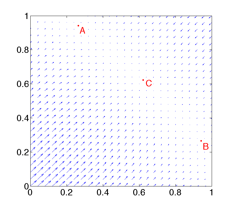
Figure 1. Vector field of Equation (3.4) with $b=0.25$. $A$ and $B$ are stable equilibriums and $C$ is a saddle point.

Remark 3.5.

Besides the toggle switch model in Example 3.2, many other biological models, including biochemical oscillation systems [47], genetic circuits [48], gene regulatory networks [24], and cell cycle network [34], are known to have similar quasi-potential landscape, hence H¹) is satisfied by all these systems. Also see [49, 1] for theoretical studies of quasi-potential functions in biological systems and [50, 49, 40, 22] for numerical computation methods of the quasi-potential function.

3.2. Concentration of stationary measures near the global attractor

Let $L_{1}$ be as in H⁰) and denote $\gamma_{0}$ as the Lyapunov constant of $W$. The following lemma is straightforward from the $C^{2}$ smoothness of $W$.

Lemma 3.2.

Assume H⁰). Then there are positive constants $\kappa,L_{1},L_{2},K_{1},K_{2}$ such that

$$-\kappa|\nabla W(x)|^{2}\leq\nabla W(x)\cdot f(x)\leq-\gamma_{0}|\nabla W(x)|^{2},$$

$$L_{1}\mathrm{dist}^{2}(x,\mathcal{A})\leq W(x)\leq L_{2}\mathrm{dist}^{2}(x,\mathcal{A}),$$

$$K_{1}\mathrm{dist}(x,\mathcal{A})\leq|\nabla W(x)|\leq K_{2}\mathrm{dist}(x,\mathcal{A}),$$

$x\in\mathcal{N}$.

Below, for any bounded set $A\subset\mathbb{R}^{n}$ and $r>0$, we denote $B(A,r):=\{x\in\mathbb{R}^{n}\,:\,\mathrm{dist}(x,A)\leq r\}$ as the $r$-neighborhood of $A$. The following theorems give new estimations in the vicinity of $\mathcal{A}$.

Theorem 3.3.

If both H⁰) and H¹) hold, then for any $0<\delta\ll 1$ there exist constants $\epsilon_{0},M>0$ such that

$$\mu_{\epsilon}(B(\mathcal{A},M\epsilon))\geq 1-\delta,$$

whenever $\epsilon\in(0,\epsilon_{0})$.

Proof.

Fix a $\rho_{0}>0$ such that $\Omega_{\rho_{0}}(W)\subset\mathcal{N}$ and $\Gamma_{\rho_{0}}\cap\mathcal{A}=\emptyset$. Then by Lemma  3.1 there are constants $\epsilon_{0},C_{1}>0$ such that $\mu_{\epsilon}(\mathcal{N}\setminus\Omega_{\rho_{0}}(W))<e^{-C_{1}/\epsilon^{2}}$, $\epsilon\in(0,\epsilon_{0})$. Since by H¹), $\mu_{\epsilon}(\mathbb{R}^{n}\setminus\mathcal{N})=o(\epsilon^{2})$, $0<\epsilon\ll 1$, we only need to estimate $\mu_{\epsilon}(\Omega_{\rho_{0}}(W))$.

For any given $0<\tilde{\rho}_{0}<\rho_{0}$ and any $0<\Delta\rho\ll 1$, consider the following $C^{2}$ cut-off function

$$\phi(\rho)=\left\{\begin{array}[]{ll}0,&\rho\leq\tilde{\rho}_{0}\\ \frac{3}{\Delta\rho^{4}}(\rho-\tilde{\rho}_{0})^{5}-\frac{8}{\Delta\rho^{3}}(\rho-\tilde{\rho}_{0})^{4}+\frac{6}{\Delta\rho^{2}}(\rho-\tilde{\rho}_{0})^{3},&\tilde{\rho}_{0}<\rho<\tilde{\rho}_{0}+\Delta\rho\\ \rho-\tilde{\rho}_{0},&\rho\geq\tilde{\rho}_{0}+\Delta\rho.\end{array}\right.$$

Let $u=u_{\epsilon}$ be a density function of $\mu_{\epsilon}$. It follows from Theorem  2.2 that

$$\int_{\Omega_{\rho_{0}}(W)}\phi^{\prime}(W(x))\left(\sum_{i,j=1}^{n}\frac{1}{2}\epsilon^{2}a_{ij}(x)\partial^{2}_{ij}W(x)+\sum_{i=1}^{n}f_{i}(x)\partial_{i}W(x)\right)u(x)\mathrm{d}x$$

$$\quad+\int_{\Omega_{\rho_{0}}(W)}\phi^{\prime\prime}(W(x))\left(\sum_{i,j=1}^{n}\frac{1}{2}\epsilon^{2}a_{ij}(x)\partial_{i}W(x)\partial_{j}W(x)\right)u(x)\mathrm{d}x$$

(3.6) $$= \int_{\Gamma_{\rho_{0}}(W)}\left(\sum_{i=1}^{n}\sum_{j=1}^{n}\frac{1}{2}\epsilon^{2}a_{ij}(x)\partial_{i}W(x)\nu_{j}(x)\right)u(x)\mathrm{d}x\geq 0,$$

where $\nu_{j}=\frac{\partial W_{j}}{|\nabla W|}$ for each $j$.

To estimate the first term on the left hand side of (3.6), we note by definition of $\phi(\rho)$ that

$$\int_{\Omega_{\rho_{0}}(W)}\phi^{\prime}(W(x))\left(\sum_{i,j=1}^{n}\frac{1}{2}\epsilon^{2}a_{ij}(x)\partial^{2}_{ij}W(x)+\sum_{i=1}^{n}f_{i}(x)\partial_{i}W(x)\right)u(x)\mathrm{d}x$$

$$= \int_{\Omega_{\rho_{0}}(W)\backslash\Omega_{\tilde{\rho}_{0}(W)}}\phi^{\prime}(W(x))\left(\sum_{i,j=1}^{n}\frac{1}{2}\epsilon^{2}a_{ij}(x)\partial^{2}_{ij}W(x)+\sum_{i=1}^{n}f_{i}(x)\partial_{i}W(x)\right)u(x)\mathrm{d}x.$$

Denote

$$\bar{\sigma} = n^{2}\max_{1\leq i,j\leq n,x\in U_{\rho_{0}(W)}}|a_{ij}(x)|,$$

$$D = \max_{1\leq i,j\leq n,x\in U_{\rho_{0}}(W)}\partial^{2}_{ij}W(x)$$

and let $M_{1}=D\bar{\sigma}/\gamma_{0}K^{2}_{1}$, where $\gamma_{0}$ and $K_{1}$ are constants in Lemma 3.2. Let $\epsilon_{1}>0$ be such that $B(\mathcal{A},\sqrt{M_{1}}\epsilon)\subset\Omega_{\rho_{0}}(W)$ for all $0<\epsilon<\epsilon_{1}$. Then

$$\sum_{i,j=1}^{n}\frac{1}{2}\epsilon^{2}a_{ij}(x)\partial^{2}_{ij}W(x)\leq\frac{\gamma_{0}}{2}|\nabla W(x)|^{2},$$

for all $x$ with $\mathrm{dist}(x,\mathcal{A})>\sqrt{M_{1}}\epsilon$ and $\epsilon\in(0,\epsilon_{1})$. It follows from the property of strong Lyapunov function that

$$\sum_{i,j=1}^{n}\frac{1}{2}\epsilon^{2}a_{ij}(x)\partial^{2}_{ij}W(x)+\sum_{i=1}^{n}f_{i}(x)\partial_{i}W(x)\leq-\frac{1}{2}\gamma_{0}|\nabla W(x)|^{2}$$

for all $x$ with $\mathrm{dist}(x,\mathcal{A})>\sqrt{M_{1}}\epsilon$ and $\epsilon\in(0,\epsilon_{1})$. Let ${\mathcal{D}}_{0}=\Omega_{\rho_{0}}(W)\backslash\Omega_{\tilde{\rho}_{0}+\Delta\rho}$ and $\mathcal{D}=\Omega_{\tilde{\rho}_{0}+\Delta\rho}(W)\backslash\Omega_{\tilde{\rho}_{0}}$. By Lemma 3.2, we also have

$$\min_{{\mathcal{D}}_{0}}|\nabla W(x)|^{2} \geq K_{1}^{2}\min_{{\mathcal{D}}_{0}}\mathrm{dist}^{2}(x,\mathcal{A})\geq\frac{K_{1}^{2}}{L_{2}}\min_{{\mathcal{D}}_{0}}W(x)=\frac{K_{1}^{2}}{L_{2}}(\tilde{\rho}_{0}+\Delta\rho)$$

$$\geq \frac{K_{1}^{2}}{L_{2}}\max_{D}W(x)\geq\frac{K_{1}^{2}L_{1}}{L_{2}}\max_{\mathcal{D}}\mathrm{dist}^{2}(x,\mathcal{A})$$

$$\geq \frac{K_{1}^{2}L_{1}}{K_{2}^{2}L_{2}}\max_{\mathcal{D}}|\nabla W(x)|^{2}=:C_{1}\max_{\mathcal{D}}|\nabla W(x)|^{2},$$

where $K_{1},K_{2},L_{1},L_{2}$ are as in Lemma 3.2. Therefore,

$$\int_{\Omega_{\rho_{0}}(W)\backslash\Omega_{\tilde{\rho}_{0}}(W)}\phi^{\prime}(W(x))\left(\sum_{i,j=1}^{n}\frac{1}{2}\epsilon^{2}a_{ij}(x)\partial^{2}_{ij}W(x)+\sum_{i=1}^{n}f_{i}(x)\partial_{i}W(x)\right)u(x)\mathrm{d}x$$

$$\leq -\gamma_{0}\int_{\Omega_{\rho_{0}}(W)\backslash\Omega_{\tilde{\rho}_{0}}(W)}\phi^{\prime}(W(x))|\nabla W(x)|^{2}u(x)\mathrm{d}x$$

$$\leq -\gamma_{0}\int_{\Omega_{\rho_{0}}(W)\backslash\Omega_{\tilde{\rho}_{0}+\Delta\rho}(W)}|\nabla W(x)|^{2}u(x)\mathrm{d}x$$

$$\leq -\gamma_{0}\min_{{\mathcal{D}}_{0}}|\nabla W(x)|^{2}\int_{\Omega_{\rho_{0}}(W)\backslash\Omega_{\tilde{\rho}_{0}+\Delta\rho}(W)}u(x)\mathrm{d}x$$

$$\leq -\gamma_{0}C_{1}\max_{\mathcal{D}}|\nabla W(x)|^{2}\mu_{\epsilon}(\Omega_{\rho_{0}}(W)\backslash\Omega_{\tilde{\rho}_{0}+\Delta\rho}(W)).$$

Note that $|\phi^{\prime\prime}(x)|\leq 4$. The second term on the left hand side of (3.6) simply satisfies the following estimate:

(3.8) $$\int_{\Omega_{\rho_{0}}(W)}\phi^{\prime\prime}(W(x))\sum_{i,j=1}^{n}\frac{1}{2}\epsilon^{2}a_{ij}(x)\partial_{i}W(x)\partial_{j}W(x)u\mathrm{d}x$$

$$= \int_{\Omega_{\tilde{\rho}_{0}+\Delta\rho}(W)\backslash\Omega_{\tilde{\rho}_{0}}(W)}\phi^{\prime\prime}(W(x))\sum_{i,j=1}^{n}\frac{1}{2}\epsilon^{2}a_{ij}(x)\partial_{i}W(x)\partial_{j}W(x)u\mathrm{d}x$$

$$\leq \frac{2}{\Delta\rho}\epsilon^{2}\bar{\lambda}\max_{\mathcal{D}}{|\nabla W(x)|^{2}\mu_{\epsilon}(\Omega_{\tilde{\rho}_{0}+\Delta\rho}\backslash\Omega_{\tilde{\rho}_{0}}}),$$

where $\bar{\lambda}=\sup_{x\in\Omega_{\rho_{0}}(W)}\lambda_{M}(x)$ with $\lambda_{M}(x)$ being the largest eigenvalue of matrix $A(x)$ for each $x\in\Omega_{\rho_{0}}(W)$.

It now follows from (3.6)-(3.8) that

(3.9) $$-\gamma_{0}C_{1}\mu(\Omega_{\rho_{0}}(W)\backslash\Omega_{\tilde{\rho}_{0}+\Delta\rho}(W))+\frac{2}{\Delta\rho}\epsilon^{2}\bar{\lambda}\mu(\Omega_{\tilde{\rho}_{0}+\Delta\rho}(W)\backslash\Omega_{\tilde{\rho}_{0}}(W))\geq 0.$$

Let $\rho_{1}=L_{2}M_{1}\epsilon^{2}$. We have by Lemma 3.2 that $B(\mathcal{A},\sqrt{M_{1}}\epsilon)\subset\Omega_{\rho_{1}}$. Consider function $F(\rho)=\mu_{\epsilon}(\Omega_{\rho_{0}}(W)\backslash\Omega_{\rho}(W))$, $\rho\in[\rho_{1},\rho_{0}]$. Since $\tilde{\rho}_{0}$ is arbitrary, (3.9) with $\rho$ in place of $\tilde{\rho}_{0}$ becomes

$$-\gamma_{0}C_{1}F(\rho+\Delta\rho)+\frac{2}{\Delta\rho}\epsilon^{2}\bar{\lambda}(F(\rho)-F(\rho+\Delta\rho))\geq 0,\qquad\rho\in[\rho_{1},\rho_{0}].$$

Taking limit $\Delta\rho\rightarrow 0$ in the above yields

$$\gamma_{0}C_{1}F(\rho)+2\epsilon^{2}\bar{\lambda}F^{\prime}(\rho)\leq 0.$$

Hence, by Gronwall’s inequality, we have

(3.10) $$F(\rho)\leq F(\rho_{1})e^{-\frac{\gamma_{0}C_{1}}{2\epsilon^{2}\bar{\lambda}}(\rho-\rho_{1})},\quad\rho\in[\rho_{1},\rho_{0}]\,.$$

For a given sufficiently small $\delta>0$, we let

$$M_{2}=L_{2}M_{1}-\frac{2\bar{\lambda}}{\gamma_{0}}C_{1}\log\frac{\delta}{2}\,.$$

Then it is easy to see from (3.10) that

(3.11) $$F(M_{2}\epsilon^{2})=\mu_{\epsilon}(\Omega_{\rho_{0}}(W))-\mu_{\epsilon}(\Omega_{M_{2}\epsilon^{2}}(W))\leq\frac{\delta}{2},$$

whenever $\epsilon<\epsilon_{2}=:\frac{\rho_{0}}{M_{2}}$.

Since $\mu_{\epsilon}(\mathbb{R}^{n}\setminus\Omega_{\rho_{0}}(W))<e^{-C_{0}/\epsilon^{2}}+o(\epsilon^{2})$, there exists an $\epsilon_{3}>0$ such that $\mu_{\epsilon}(\mathbb{R}^{n}\setminus\Omega_{\rho_{0}}(W))<\frac{\delta}{2}$, i.e., $\mu_{\epsilon}(\Omega_{\rho_{0}}(W))>1-\frac{\delta}{2}$, for all $\epsilon\in(0,\epsilon_{3})$. Hence by (3.11),

$$\mu_{\epsilon}(\Omega_{M_{2}\epsilon^{3}}(W))\geq 1-\delta,\quad 0<\epsilon<\epsilon_{0},$$

where $\epsilon_{0}=\min\{\epsilon_{1},\epsilon_{2},\epsilon_{3}\}$.

Let $M=\sqrt{\frac{M_{2}}{L_{1}}}$. Then by Lemma 3.2,

$$\Omega_{M_{2}\epsilon^{2}}(W)\subset B(\mathcal{A},M\epsilon),$$

and therefore,

$$\mu_{\epsilon}(B(\mathcal{A},M\epsilon))\geq\mu_{\epsilon}(\Omega_{M_{2}\epsilon^{2}}(W))\geq 1-\delta,\quad 0<\epsilon<\epsilon_{0}.$$

This completes the proof. ∎

Remark 3.6.

1) From the proof of Theorem  3.3, one sees that the constant $M$ grows in a logarithm rate as $\delta$ decreases. In fact, for a fixed small $\epsilon$, we have

$$\lim_{\delta\rightarrow 0}\frac{M}{\sqrt{-\log\delta}}=C$$

for some finite constant $C$.

2) Theorem  3.3 does not follow from Lemma  2.1 directly simply because for any constant $M>0$ the Lyapunov constant of $W$ in the set $\Omega_{M\epsilon^{2}}(W)$ becomes O($\epsilon)$ instead of being O(1).

Next we estimate the lower bound of concentration of $\mu_{\epsilon}$.

Lemma 3.3.

There is a constant $r_{0}>0$ such that $\sum_{i,j=1}^{n}a_{ij}(x)W_{ij}(x)$ is uniformly positive in $B(\mathcal{A},r_{0})$.

Proof.

First we note that the Hessian matrix $\mathbf{H}(x):=(W_{ij}(x))$ of $W(x)$ must be positive semidefinite for all $x\in\mathcal{A}$. For otherwise, there is $x_{0}\in\mathcal{A}$ such that $\mathbf{H}(x_{0})$ has negative eigenvalue. It then follows from the $C^{2}$ smoothness of $W(x)$ that $W(x)$ must take a negative value at some $x\in\mathcal{N}$ where $x-x_{0}$ is an eigenvector corresponding to the negative eigenvalue of $\mathbf{H}(x_{0})$. This is a contradiction because $W(x)$ must be everywhere non-negative in $\mathcal{N}$.

Since $A(x)=(a_{ij}(x))$ is everywhere positive definite in $\bar{\mathcal{N}}$, all its eigenvalues in $\mathcal{N}$ are bounded below by a positive constant $\lambda_{0}$. For any $x_{0}\in\mathcal{A}$, since $W(x)\geq L_{1}\mathrm{dist}(x,\mathcal{A})^{2}$, $x\in\mathcal{N}$, Taylor expansion of $W$ at $x_{0}$ shows that at least one eigenvalue of $\mathbf{H}(x_{0})$ must be positive. Consequently,

$$\sum_{i,j=1}^{n}a_{ij}(x_{0})W_{ij}(x_{0})=\mathrm{trace}(A(x_{0})\mathbf{H}(x_{0}))\geq\lambda_{0}\mathrm{trace}(\mathbf{H}(x_{0}))>0.$$

The proposition simply follows from the continuity of $\sum_{i,j=1}^{n}a_{ij}(x)W_{ij}(x)$.

∎

Theorem 3.4.

If both H⁰) and H¹) hold, then

$$\lim_{\epsilon\rightarrow 0}\mu_{\epsilon}(\{x:\,\epsilon^{1+\alpha}\leq\mathrm{dist}(x,\mathcal{A})\leq\epsilon^{1-\alpha}\})=1$$

for any $0<\alpha<1$.

Proof.

By Lemma  3.2, there is a constant $\epsilon_{0}>0$ such that both $\{x\,|\mathrm{dist}(x,\mathcal{A})\leq\epsilon^{1-\alpha}\}\subseteq\Omega_{\epsilon^{2-\alpha}(W)}$ and $\{x\,|\mathrm{dist}(x,\mathcal{A})\leq\epsilon^{1+\alpha}\}\supseteq\Omega_{\epsilon^{2+3\alpha}(W)}$ hold for all $\epsilon\in(0,\epsilon_{0})$. Thus it suffices to prove that

(3.12) $$\lim_{\epsilon\rightarrow 0}\mu_{\epsilon}(\Omega_{\epsilon^{2+\delta}}(W))=0,$$

(3.13) $$\lim_{\epsilon\rightarrow 0}\mu_{\epsilon}(\Omega_{\epsilon^{2-\delta}}(W))=1.$$

for any fixed $\delta>0$.

Equation (3.13) follows from Theorem  3.3 immediately. We will prove equation (3.12).

Fix a $\rho_{0}>0$ such that $\Omega_{\rho_{0}}(W)\subseteq\mathcal{N}$ and $\Gamma_{\rho_{0}}\cap\mathcal{A}=\emptyset$. Consider $f(\rho)=\mu_{\epsilon}(\Omega_{\rho}(W))$ for $\rho\in[0,\rho_{0}]$. Assume, for the sake of contradiction, that there is a constant $\sigma>0$ such that $f(\epsilon^{2+\delta})\geq\sigma>0$ for any sufficient small $\epsilon>0$.

We have by Theorem  2.3 that

(3.14) $$\int_{\Gamma_{\rho}(W)}\frac{u(x)}{|\nabla W(x)|}\mathrm{d}s=f^{\prime}(\rho)\,.$$

Let $\bar{\lambda}=\sup_{x\in\Omega_{\rho^{0}}(W)}\lambda_{M}(x)$ with $\lambda(x)$ being the largest eigenvalue of matrix $A(x)$ for each $x\in\Omega_{\rho^{0}}(W)$. Let $u=u_{\epsilon}$ be the density function of $\mu_{\epsilon}$. It follows from Lemma 3.2 and (3.14) that for each $0<\rho<\rho_{0}$, inequality

$$\int_{\Gamma_{\rho}(W)}\frac{1}{2}\epsilon^{2}\left(\sum_{i,j=1}^{n}a_{ij}(x)\partial_{i}W(x)\nu_{j}(x)\right)u(x)\mathrm{d}s$$

$$= \int_{\Gamma_{\rho}(W)}\frac{1}{2}\epsilon^{2}\left(\sum_{i,j=1}^{n}a_{ij}(x)\partial_{i}W(x)\partial_{j}W(x)\right)\frac{u(x)}{|\nabla W(x)|}\mathrm{d}s$$

$$\leq \int_{\Gamma_{\rho}(W)}\frac{1}{2}\epsilon^{2}\bar{\lambda}|\nabla W(x)|^{2}\frac{u(x)}{|\nabla W(x)|}\mathrm{d}s$$

$$\leq \int_{\Gamma_{\rho}(W)}\frac{1}{2}\epsilon^{2}\bar{\lambda}\frac{K_{2}^{2}}{L_{1}}W(x)\frac{u(x)}{|\nabla W(x)|}\mathrm{d}s$$

$$\leq \epsilon^{2}C_{1}\rho f^{\prime}(\rho)$$

holds for some positive constant $C_{1}<\infty$.

By Lemma  3.2, we have the inequality

(3.15) $$\sum_{i=1}^{n}f_{i}(x)\partial_{i}W(x)\geq-\kappa|\nabla W(x)|^{2}\geq-\kappa\frac{K_{2}^{2}}{L_{1}}W(x)\,.$$

It then follows from Lemma  3.3 and (3.15) that there are positive constants $p,C_{2}$ and $\epsilon_{0}$ such that

$$\frac{1}{2}\epsilon^{2}\sum_{i,j=1}^{n}a_{ij}(x)W_{ij}(x)+\sum_{i=1}^{n}f_{i}(x)\partial_{i}W(x)\geq p\epsilon^{2}$$

for all $x\in\Omega_{C_{2}\epsilon^{2}}(W)$ and $\epsilon\in(0,\epsilon_{0})$. Without loss of generality, we make $\epsilon$ sufficiently small such that $\rho_{0}>C_{2}\epsilon^{2}$. Then for each $\rho\leq C_{2}\epsilon^{2}$ there holds

$$\int_{\Omega_{\rho}(W)}\left(\frac{1}{2}\epsilon^{2}\sum_{i,j=1}^{n}a_{ij}(x)W_{ij}(x)+\sum_{i=1}^{n}f_{i}(x)\partial_{i}W(x)\right)u\mathrm{d}x\geq pf(\rho)\epsilon^{2}\,.$$

Since by Theorem 2.2,

$$\int_{\Omega_{\rho}(W)}\left(\frac{1}{2}\epsilon^{2}\sum_{i,j=1}^{n}a_{ij}(x)W_{ij}(x)+\sum_{i=1}^{n}f_{i}(x)\partial_{i}W(x)\right)u\mathrm{d}x$$

$$= \int_{\Gamma_{\rho}(W)}\frac{1}{2}\epsilon^{2}\left(\sum_{i,j=1}^{n}a_{ij}(x)\partial_{i}W(x)\nu_{j}(x)\right)u(x)\mathrm{d}s\,.$$

we conclude that

$$pf(\rho)\epsilon^{2}\leq\epsilon^{2}C_{1}\rho f^{\prime}(\rho)$$

for each $0<\rho\leq C_{2}\epsilon^{2}$. Thus

(3.16) $$\frac{f^{\prime}(\rho)}{f(\rho)}\geq\frac{p}{C_{1}\rho}\,.$$

Integrating (3.16) from $\epsilon^{2+\delta}$ to $C_{2}\epsilon^{2}$ yields

$$\log f(C_{2}\epsilon^{2})-\log\sigma\geq\frac{p}{C_{1}}(\log C_{2}-\delta\log\epsilon)\,.$$

As $\epsilon\rightarrow 0$, we have $f(C_{2}\epsilon^{2})\rightarrow\infty$. This contradicts to the fact that $f(\rho)\leq 1$. Hence $f(\epsilon^{2+\delta})=\mu_{\epsilon}(\Omega_{\epsilon^{2+\delta}})\rightarrow 0$. This completes the proof.

∎

Remark 3.7.

Theorem  3.4 says that the density function of $\mu_{\epsilon}$ cannot be “too narrow” because almost all the mass of $\mu_{\epsilon}$ is located in the set $\{x:\,\epsilon^{1+\alpha}\leq\mathrm{dist}(x,\mathcal{A})\leq\epsilon^{1-\alpha}\}$.

3.3. Mean square displacement

The concentration of $\mu_{\epsilon}$ can be more concretely measured by the mean square displacement defined by

$$V(\epsilon)=\int_{\mathbb{R}^{n}}\mathrm{dist}^{2}(x,\mathcal{A})\mathrm{d}\mu_{\epsilon}.$$

The following theorem gives bounds of the mean square displacement.

Theorem 3.5.

If both H⁰) and H¹) hold, then there are constants $V_{1},V_{2},\epsilon_{0}>0$ independent of $\epsilon$ such that

$$V_{2}\epsilon^{2}\leq V(\epsilon)\leq V_{1}\epsilon^{2},\quad\epsilon\in(0,\epsilon_{0}).$$

Proof.

Fix a $\rho_{0}>0$ such that $\Omega_{\rho_{0}}(W)\subset\mathcal{N}$ and $\Gamma_{\rho_{0}}(W)\cap\mathcal{A}=\emptyset$. We have by condition H¹) and Lemma 3.1 that there is an $\epsilon_{0}\in(0,\epsilon^{*})$ sufficiently small such that

(3.17) $$\mu_{\epsilon}(\mathbb{R}^{n}\setminus\Omega_{\rho_{0}}(W))<\epsilon^{2},\quad\epsilon\in(0,\epsilon_{0}).$$

Consider the function

$$G(\rho)=\int_{\Omega_{\rho_{0}}\backslash\Omega_{\rho}}|\nabla W(x)|^{2}\mathrm{d}\mu_{\epsilon},\quad\rho\in[0,\rho_{0}].$$

Then it follows from Lemma 3.2 that

$$\frac{1}{K_{2}^{2}}G(0)\leq\int_{\Omega_{\rho_{0}}(W)}\mathrm{dist}^{2}(x,\mathcal{A})\mathrm{d}\mu_{\epsilon}\leq V(\epsilon)$$

$$=\int_{\Omega_{\rho_{0}}(W)}\mathrm{dist}^{2}(x,\mathcal{A})\mathrm{d}\mu_{\epsilon}+\int_{\mathbb{R}^{n}\backslash\Omega_{\rho_{0}}(W)}\mathrm{dist}^{2}(x,\mathcal{A})\mathrm{d}\mu_{\epsilon}$$

$$\leq\frac{1}{K_{1}^{2}}G(0)+\int_{\mathbb{R}^{n}\backslash\Omega_{\rho_{0}}(W)}\mathrm{dist}^{2}(x,\mathcal{A})\mathrm{d}\mu_{\epsilon},$$

where $K_{1},K_{2}$ are as in Lemma 3.2.

We first estimate an upper bound of $G(0)$ in term of $\epsilon^{2}$. Let $F(\rho)=\mu_{\epsilon}(\Omega_{\rho_{0}}(W)\backslash\Omega_{\rho}(W))$. Then it follows from equation (3.10) that

(3.18) $$F(\rho)\leq F(\rho_{1})e^{-\frac{2\gamma_{0}C_{1}}{\epsilon^{2}\bar{\lambda}}(\rho-\rho_{1})}\leq e^{-\frac{2\gamma_{0}C_{1}}{\epsilon^{2}\bar{\lambda}}(\rho-\rho_{1})},\quad\rho\in(\rho_{1},\rho_{0}),$$

for all $0<\epsilon\ll 1$, where $C_{1},\bar{\lambda},\gamma_{0}$ are constants independent of $\epsilon$ and $\rho_{1}=C_{2}\epsilon^{2}$ for some constant $C_{2}$ independent of $\epsilon$. Since by Lemma 3.2, $|\nabla W|^{2}\leq K_{2}^{2}\rho/L_{1}$, we have by (3.18) and Theorem  2.3 that

$$\int_{\Omega_{\rho_{0}}(W)\backslash\Omega_{\rho_{1}}(W)}|\nabla W(x)|^{2}\mathrm{d}\mu_{\epsilon}\leq-\int_{\rho_{1}}^{\rho_{0}}\frac{K_{2}^{2}}{L_{1}}\rho F^{\prime}(\rho)\mathrm{d}\rho$$

$$= \left.-\frac{K_{2}^{2}}{L_{1}}\rho F(\rho)\right|^{\rho_{0}}_{\rho_{1}}+\frac{K_{2}^{2}}{L_{1}}\int_{\rho_{1}}^{\rho_{0}}F(\rho)\mathrm{d}\rho$$

$$\leq \frac{K_{2}^{2}}{L_{1}}\rho_{1}F(\rho_{1})+\frac{K_{2}^{2}}{L_{1}}\int_{\rho_{1}}^{\infty}e^{-\frac{2\gamma_{0}C_{1}}{\epsilon^{2}\bar{\lambda}}s}\mathrm{d}s\leq\frac{K_{2}^{2}}{L_{1}}(C_{2}\epsilon^{2}+\frac{\bar{\lambda}\epsilon^{2}}{2\gamma_{0}C_{1}}e^{-\frac{2\gamma_{0}C_{1}\rho_{1}}{\epsilon^{2}\bar{\lambda}}}):=E_{2}\epsilon^{2}$$

for all $0<\epsilon\ll 1$. By a simple calculation, we also have

$$\int_{\Omega_{\rho_{1}}(W)}|\nabla W(x)|^{2}\mathrm{d}\mu_{\epsilon}\leq M_{2}\epsilon^{2}$$

as $0<\epsilon\ll 1$, where $M_{2}>0$ is a constant independent of $\epsilon$. Thus,

(3.19) $$G(0)=\int_{\Omega_{\rho_{0}}(W)}|\nabla W(x)|^{2}\mathrm{d}\mu_{\epsilon} = \int_{\Omega_{\rho_{0}(W)\setminus\Omega_{\rho_{1}}(W)}}|\nabla W(x)|^{2}\mathrm{d}\mu_{\epsilon}+\int_{\Omega_{\rho_{1}}(W)}|\nabla W(x)|^{2}\mathrm{d}\mu_{\epsilon}$$

$$\leq (E_{2}+M_{2})\epsilon^{2},\,\quad 0<\epsilon\ll 1.$$

Next, we estimate an upper bound of $\int_{\mathbb{R}^{n}\backslash\Omega_{\rho_{0}}(W)}\mathrm{dist}^{2}(x,\mathcal{A})\mathrm{d}\mu_{\epsilon}$. Let $R_{0}>0$ be as in H¹), i.e.,

$$\mu_{\epsilon}({\mathbb{R}}^{n}\setminus B(0,r))\leq e^{-\frac{r^{p}}{\epsilon^{2}}},\quad r\geq R_{0},$$

for all $\epsilon\in(0,\epsilon_{*})$. Without loss of generality, we may assume that $R_{0}$ is sufficiently large such that

$$\mathrm{dist}(x,\mathcal{A})<2|x|,\quad|x|\geq R_{0}.$$

Then

$$\int_{\mathbb{R}^{n}\backslash B(0,R_{0})}\mathrm{dist}^{2}(x,\mathcal{A})\mathrm{d}\mu_{\epsilon} \leq \int_{\{|x|>R_{0}\}}4|x|^{2}u\mathrm{d}x\leq 4\sum_{k=k_{0}}^{\infty}e^{-\frac{k^{p}}{\epsilon^{2}}}(k+1)^{n+2}C(n)$$

$$\leq 4e^{-\frac{k_{0}^{p}}{\epsilon^{2}}}\sum_{k=0}^{\infty}e^{-\frac{k^{p}}{\epsilon_{0}^{2}}}(k+k_{0}+1)^{n+2}C(n)\leq C_{5}e^{-\frac{k_{0}^{p}}{\epsilon^{2}}}$$

for all $\epsilon\in(0,\epsilon_{*})$, where $C(n)$ is the volume of the unit sphere in $\mathbb{R}^{n}$, $k_{0}$ is the largest integer smaller than $R_{0}$, and $C_{5}$ is a constant independent of $\epsilon$. Thus, we can make $\epsilon_{0}$ sufficiently small such that

(3.20) $$\int_{\mathbb{R}^{n}\backslash B(0,R_{0})}\mathrm{dist}^{2}(x,\mathcal{A})\mathrm{d}\mu_{\epsilon}<\epsilon^{2},\quad\epsilon\in(0,\epsilon_{0}).$$

Using (3.17), we can make $\epsilon_{0}$ further small if necessary such that

(3.21) $$\int_{B(0,R_{0})\backslash\Omega_{\rho_{0}}(W)}\mathrm{dist}^{2}(x,\mathcal{A})\mathrm{d}\mu_{\epsilon}<\epsilon^{2},\quad\epsilon\in(0,\epsilon_{0}).$$

It now follows from (3.20) and (3.21) that

$$\int_{\mathbb{R}^{n}\backslash\Omega_{\rho_{0}}(W)}\mathrm{dist}^{2}(x,\mathcal{A})\mathrm{d}\mu_{\epsilon}$$

$$= \int_{\mathbb{R}^{n}\backslash B(0,R_{0})}\mathrm{dist}^{2}(x,\mathcal{A})\mathrm{d}\mu_{\epsilon}+\int_{B(0,R_{0})\backslash\Omega_{\rho_{0}}(W)}\mathrm{dist}^{2}(x,\mathcal{A})\mathrm{d}\mu_{\epsilon}<2\epsilon^{2}$$

for all $\epsilon\in(0,\epsilon_{0})$. This, when combining with (3.19), yields that

$$V(\epsilon)\leq(2+\frac{E_{2}}{K_{1}^{2}})\epsilon^{2}:=V_{1}\epsilon^{2},\quad 0<\epsilon\ll 1.$$

Finally, we estimate a lower bound of $V(\epsilon)$. For each $\epsilon\in(0,\epsilon^{*})$, let $u=u_{\epsilon}$ be a density function of $\mu_{\epsilon}$. Then by Theorem  2.2

$$\int_{\Omega_{\rho}(W)}\left(\frac{1}{2}\epsilon^{2}\sum_{i,j=1}^{n}a_{ij}(x)W_{ij}(x)+\sum_{i=1}^{n}f_{i}(x)\partial_{i}W(x)\right)u(x)\mathrm{d}x$$

$$= \int_{\Gamma_{\rho}(W)}\frac{1}{2}\epsilon^{2}\left(\sum_{i,j=1}^{n}a_{ij}(x)\partial_{i}W(x)\nu_{j}(x)\right)u(x)\mathrm{d}s,\quad\rho\in(0,\rho_{0}).$$

Let $r_{0}$ be as in Lemma 3.3 and fix a $\rho_{*}\in(0,\rho_{0})$ such that $\Omega_{\rho_{*}}(W)\subset B(\mathcal{A},r_{0})$. Since $F(\rho_{0})=0$, we have by (3.18) and mean value theorem that there is a $\rho^{*}\in(\rho_{*},\rho_{0})$ such that $F^{\prime}(\rho^{*})\leq e^{-\frac{\beta}{\epsilon^{2}}}(\rho_{0}-\rho_{*})^{-1}$ as $0<\epsilon<\epsilon_{0}$, where $\beta=\frac{2\gamma_{0}C_{1}}{\bar{\lambda}}(\rho_{*}-\rho_{1})$. By H¹) and Lemma 3.1, we can make $\epsilon_{0}$ further small if necessary such that $\mu_{\epsilon}(\Omega_{\rho_{*}}(W))\geq 1-o(\epsilon^{2})$ as $\epsilon\in(0,\epsilon_{0})$. It follows from Lemma 3.3 that

(3.23) $$\int_{\Omega_{\rho^{*}}(W)}\frac{1}{2}\epsilon^{2}\sum_{i,j=1}^{n}a_{ij}(x)W_{ij}(x)u(x)\mathrm{d}x\geq\int_{\Omega_{\rho_{*}}(W)}\frac{1}{2}\epsilon^{2}\sum_{i,j=1}^{n}a_{ij}(x)W_{ij}(x)u(x)\mathrm{d}x\geq C_{4}\epsilon^{2}$$

as $0<\epsilon<\epsilon_{0}$, where $C_{4}>0$ is a constant independent of $\epsilon$. By Lemma 3.2, we also have

(3.24) $$\int_{\Omega_{\rho^{*}}(W)}\sum_{i=1}^{n}f_{i}(x)\partial_{i}W(x)u\mathrm{d}x\geq-\kappa\int_{\Omega_{\rho^{*}}(W)}|\nabla W(x)|^{2}u(x)\mathrm{d}x\geq-\kappa G(0).$$

Let $C_{5}=\frac{1}{2}\sup_{x\in\mathcal{N}}\sum_{i,j=1}^{n}a_{ij}\partial_{i}W\partial_{j}W$ and assume without loss of generality that $C_{5}e^{-\frac{\beta}{\epsilon^{2}}}(\rho_{0}-\rho_{*})^{-1}<C_{4}/2$, $\epsilon\in(0,\epsilon_{0})$. It follows from Theorem 2.3 that

$$\int_{\Gamma_{\rho^{*}}(W)}\frac{1}{2}\epsilon^{2}\left(\sum_{i,j=1}^{n}a_{ij}(x)\partial_{i}W(x)\nu_{j}(x)\right)u(x)\mathrm{d}s$$

$$= \int_{\Gamma_{\rho^{*}}(W)}\frac{1}{2}\epsilon^{2}(\sum_{i,j=1}^{n}a_{ij}(x)\partial_{i}W(x)\partial_{j}W(x))\frac{u(x)}{|\nabla W(x)|}\mathrm{d}s$$

$$\leq \epsilon^{2}C_{5}\int_{\Gamma_{\rho^{*}}(W)}\frac{u(x)}{|\nabla W(x)|}\mathrm{d}s=\epsilon^{2}C_{5}F^{\prime}(\rho^{*})$$

(3.26) $$\leq \epsilon^{2}C_{5}e^{-\frac{\beta}{\epsilon^{2}}}(\rho_{0}-\rho_{*})^{-1}\leq\frac{C_{4}}{2}\epsilon^{2},$$

as $\epsilon\in(0,\epsilon_{0})$. Now, (3.3)-(3.26) yield

$$G(0)\geq\frac{C_{4}}{2\kappa}\epsilon^{2},$$

which implies

$$V(\epsilon)\geq\frac{C_{4}}{2\kappa K_{2}^{2}}\epsilon^{2}:=V_{2}\epsilon^{2}$$

as $\epsilon\in(0,\epsilon_{0})$. This completes the proof. ∎

Remark 3.8.

The mean square displacement is a natural extension of the variance. Consider $\mathcal{A}_{1}=\{0\}$ and the Gaussian measure $\nu_{\epsilon}$ with mean $0$ and variance $\epsilon^{2}$. Then it is easy to see that Theorems 3.4,  3.5 hold for $\nu_{\epsilon}$ and $\mathcal{A}_{1}$. This is to say that, by assuming H⁰) and H¹), the concentration of $\mu_{\epsilon}$ is Gaussian-like.

4. Entropy-dimension relationship

In this section, we will investigate the connection between the differential entropy of stationary measures of (2.1) and the dimension of $\mathcal{A}$. This connection will be used in the second part of the series.

Let $\mu$ be a probability measure on $\mathbb{R}^{n}$ with a density function $\xi(x)$. We recall that the relative entropy of $\mu$ with respect to Lebusgue measure, or the differential entropy of $\mu$ is defined as

(4.1) $$\mathcal{H}(\mu)=-\int_{\mathbb{R}^{n}}\xi(x)\log\xi(x)\mathrm{d}x\,.$$

4.1. Regularity of sets and measures

To establish the connection between the entropy of a stationary measure $\mu_{\epsilon}$ of (2.1) and the dimension of $\mathcal{A}$, we will require $\mathcal{A}$ be a regular set and $\mu_{\epsilon}$ be a regular measure with respect to $\mathcal{A}$.

A set $A\subset\mathbb{R}^{n}$ is called a regular set if

$$\limsup_{r\rightarrow 0}\frac{\log m(B(A,r))}{\log r}=\liminf_{r\rightarrow 0}\frac{\log m(B(A,r))}{\log r}=n-d$$

for some $d\geq 0$, where $m(\cdot)$ denotes the Lebesgue measure on $\mathbb{R}^{n}$. It is easy to check that $d$ is the Minkowski dimension of $A$. Regular sets form a large class that includes smooth manifolds and even fractal sets like Cantor sets. However, not all measurable sets are regular (see [39] for details).

Assume that (1.1) admits a global attractor $\mathcal{A}$ and the Fokker-Planck equation (2.1) admits a stationary measure $\mu_{\epsilon}$ for each $\epsilon\in(0,\epsilon_{*})$. The family $\{\mu_{\epsilon}\}$ of stationary measures is said to be regular with respect to $\mathcal{A}$ if for any $\delta>0$ there are constants $K$, $C$ and a family of approximate funtions $u_{K,\epsilon}$ supported on $B(\mathcal{A},K\epsilon)$ such that for all $\epsilon\in(0,\epsilon^{*})$,

• (4.2) $$\inf_{B(\mathcal{A},K\epsilon)}(u_{K,\epsilon}(x))\geq C\sup_{B(\mathcal{A},K\epsilon)}(u_{K,\epsilon}(x))\,;$$

  and

• $$\|u_{\epsilon}(x)-u_{K,\epsilon}(x)\|_{L^{1}}\leq\delta\,.$$

The following propositions give some examples of regular stationary measures.

Proposition 4.1.

Assume equation (1.2) has the form

(4.3) $$\mathrm{d}X_{t}=-\nabla U(X)\mathrm{d}t+\epsilon\mathrm{d}W_{t},\quad X\in{\mathbb{R}}^{n},$$

where $U\in C^{2}({\mathbb{R}}^{n})$ is such that $U(x)\geq\beta\log|x|$ as $|x|\gg 1$ for some positive constant $\beta$. Then the family of stationary measures of the Fokker-Planck equations associated with (4.3) is regular with respect to $\mathcal{A}$ as $0<\epsilon\ll 1$.

Proof.

For each $\epsilon\ll 1$, the Fokker-Planck equation associated with (4.3) admits a unique stationary measure $\mu_{\epsilon}$ which actually coincides with the Gibbs measure with density

(4.4) $$\frac{1}{K}e^{-\frac{U(x)}{\epsilon^{2}}}\,,$$

where $K$ is the normalizer (see e.g. [25] and references therein). The regularity of the family $\{\mu_{\epsilon}\}$ thus follows easily from (4.4) and the definition. ∎

Proposition 4.2.

Consider (1.2) and assume that H¹) holds. If $\mathcal{A}$ is an equilibrium, then the the family $\mu_{\epsilon}$ is regular with respect to $\mathcal{A}$.

Proof.

Without loss of generality, we assume that $\mathcal{A}=\{0\}$. It follows from H¹) and the WKB expansion (see [33, 9, 8]) that there is a function $W\in C^{2}({\mathbb{R}}^{n})$, called quasi-potential function, such that the density function of $\mu_{\epsilon}$ for each $\epsilon\in(0,\epsilon^{*})$ has the form

(4.5) $$\frac{1}{K}z(x)e^{-\frac{W(x)}{\epsilon^{2}}}+o(\epsilon^{2})\,,$$

where $K$ is the normalizer and $z\in C({\mathbb{R}}^{n})$. It is easy to see that $u_{\epsilon}(x)$ is regular. The regularity of the family $\{\mu_{\epsilon}\}$ then follows from (4.5) and the definition. ∎

In many biological applications, WKB expansion as in (4.5) is assumed [36, 6, 35]. If the family of stationary measures satisfies (4.5), then it must be regular with respect to $\mathcal{A}$. However, if $\mathcal{A}$ is not an equilibrium, verifying (4.5) is difficult in general. Still, although there are some technical huddles, proving that a stationary measure is regular with respect to the global attractor is possible in many cases.

If $\mathcal{A}$ is a limit cycle on which $f$ is everywhere non-vanishing, then equation (1.2) can be linearized in the vicinity of $\mathcal{A}$. The solution of the linearized equation can be explicitly given. Therefore the density function of $\mu_{\epsilon}$ can be estimated via probabilistic approaches. We will prove in our future work that the family $\mu_{\epsilon}$ is regular with respect to the limit cycle $\mathcal{A}$. In addition, we conjecture that when H¹) holds for equation (1.2) and equation (1.1) admits an SRB measure, the family $\mu_{\epsilon}$ is regular with respect to $\mathcal{A}$ under suitable conditions.

4.2. Entropy and dimension

The main theorem of this subsection is the following entropy-dimension inequality.

Theorem 4.1.

Assume that H⁰) and H¹) hold. If $\mathcal{A}$ is a regular set, then

(4.6) $$\liminf_{\epsilon\rightarrow 0}\frac{\mathcal{H}(\mu_{\epsilon})}{\log\epsilon}\geq n-d\,,$$

where $d$ is the Minkowski dimension of $\mathcal{A}$.

To prove Theorem 4.1, the following three lemmas that estimate the integral of $u_{\epsilon}(x)\log u_{\epsilon}(x)$ are useful. The first lemma estimates the integral of $u_{\epsilon}(x)\log u_{\epsilon}(x)$ outside large spheres.

Lemma 4.1.

Let $l>0$ be a fixed constant independent of $\epsilon$. If H¹) holds, then there exist positive constants $\epsilon_{0}$, $R_{0}$ such that

$$\int_{|x|>R_{0}}u_{\epsilon}(x)\log u_{\epsilon}(x)\mathrm{d}x\geq-\epsilon^{l}\,,$$

for all $\epsilon\in(0,\epsilon_{0})$.

Proof.

It follows from H¹) that $\mu_{\epsilon}$ has the tail bounds

$$\mu_{\epsilon}(\mathbb{R}^{n}\setminus B(0,|x|))=\int_{\mathbb{R}^{n}\setminus B(0,|x|)}u_{\epsilon}(x)\mathrm{d}x\leq e^{-\frac{|x|^{p}}{\epsilon^{2}}}$$

for all $|x|>R_{0}$, where $R_{0}$ and $p$ are positive constants independent of $\epsilon$.

For each positive integer $k$, we denote $\Omega_{k}=\{x:\,k\leq|x|<k+1\}$. Let $k_{0}$ be the smallest integer that is larger than $R_{*}$. Then for each $k>k_{0}$, we have

$$\int_{\Omega_{k}}u_{\epsilon}(x)\mathrm{d}x\leq e^{-\frac{k^{p}}{\epsilon^{2}}}\,.$$

Let $\Omega_{k}=A_{k}\cup B_{k}$ where $A_{k}=\{x\in\Omega_{k}:\,u_{\epsilon}(x)\geq e^{-\frac{k^{p}}{\epsilon^{2}}}\}$, $B_{k}=\Omega_{k}\setminus A_{k}$. Since $x\log x$ decreases on the interval $(0,e^{-1})$, for sufficient small $\epsilon$ we have

$$\int_{A_{k}}u_{\epsilon}(x)\log u_{\epsilon}(x)\mathrm{d}x\geq-\frac{k^{p}}{\epsilon^{2}}\int_{A_{k}}u_{\epsilon}(x)\mathrm{d}x\geq-\frac{k^{p}}{\epsilon^{2}}e^{-\frac{k^{p}}{\epsilon^{2}}}=:a_{k}$$

and

$$\int_{B_{k}}u_{\epsilon}(x)\log u_{\epsilon}(x)\geq\int_{B_{k}}-\frac{k^{p}}{\epsilon^{2}}e^{-k^{p}/\epsilon^{2}}\mathrm{d}x\geq-\frac{\pi^{\frac{n}{2}}}{\Gamma(\frac{n}{2}+1)}k^{n}\frac{k^{p}}{\epsilon^{2}}e^{-\frac{k^{p}}{\epsilon^{2}}}=:b_{k}\,,$$

where $\Gamma(x)$ is the Gamma function.

It is easy to see that for any $l>0$ there is an $\epsilon_{0}>0$ such that

$$\sum_{k=k_{0}}^{\infty}a_{k}+b_{k}\geq-\epsilon^{l}$$

for all $\epsilon\in(0,\epsilon_{0})$. The proof is completed by letting $R_{0}=k_{0}$. ∎

The second lemma bounds the integration of $u_{\epsilon}(x)\log u_{\epsilon}(x)$ over compact sets.

Lemma 4.2.

Let $v(x)$ be a probability density function on $\mathbb{R}^{n}$ and $\Omega\subseteq\mathbb{R}^{n}$ be a Lebesgue measurable compact set. Then there is a $\delta_{0}>0$ such that for each $\delta\in(0,\delta_{0})$, if

$$\int_{\Omega}v(x)\mathrm{d}x\leq\delta$$

then

$$\int_{\Omega}v(x)\log v(x)\mathrm{d}x\geq-2\sqrt{\delta}\,.$$

Proof.

The proof only contains elementary calculations. Let $\eta=\sqrt{\delta}$ and write $\Omega$ into $\Omega=A\cup B$, where $A=\{x\in\Omega:\,v(x)>e^{-1/\eta}\}$ and $B=\Omega\setminus A$. Then for every $\eta<1$, we have

$$\int_{A}v(x)\log v(x)\mathrm{d}x\geq-\frac{1}{\eta}\int_{A}v(x)\mathrm{d}x\geq-\frac{\delta}{\eta}$$

and

$$\int_{B}v(x)\log v(x)\mathrm{d}x\geq-\frac{1}{\eta}e^{-\frac{1}{\eta}}\int_{B}\mathrm{d}x\geq-\frac{V}{\eta}e^{-\frac{1}{\eta}}\,,$$

where $V$ denotes the Lebesgue measure of $\Omega$.

Let $\delta_{0}=(\log V)^{-2}$. Then for any $\delta<\delta_{0}$, we have

$$\int_{\Omega}v(x)\log v(x)\mathrm{d}x\geq-2\sqrt{\delta}\,.$$

∎

The upper bound of $u_{\epsilon}(x)$ is estimated in the following lemma.

Lemma 4.3.

If H¹) holds, then there is a constant $\epsilon_{0}>0$ such that $u_{\epsilon}(x)\leq\epsilon^{-2n+1}$ whenever $x\in\mathbb{R}^{n}$ and $\epsilon\in(0,\epsilon_{0})$.

Proof.

We first show that there are positive constants $p$, $\epsilon_{0}$ and $R_{*}<\infty$ independent of $\epsilon$ such that

(4.7) $$u_{\epsilon}(x)\leq e^{-\frac{|x|^{p}}{2\epsilon^{2}}}$$

for every $|x|>R_{*}$ and $\epsilon\in(0,\epsilon_{0})$.

It follows from H¹) that there exist positive constants $p$, $\epsilon_{*}$ and $R_{0}$ such that

$$\mu_{\epsilon}(B(0,r))\leq e^{-\frac{r^{p}}{\epsilon^{2}}}$$

for all $r>R_{0}$ and $\epsilon\in(0,\epsilon_{*})$. For the sake of contradiction, we assume $u_{\epsilon}(x_{0})>e^{-|x_{0}|^{p}/2\epsilon^{2}}$ for some $x_{0}\in\mathbb{R}^{n}$ with $|x_{0}|>R_{0}+1$. It follows from Lemma  2.3 that there is a constant $C>0$ such that for any ball $B(x_{0},r)$ where $r<1/4$, we have

$$\sup_{B(x_{0},r)}u_{\epsilon}\leq C\inf_{B(x_{0},r)}u_{\epsilon}\,,$$

where $C=C_{0}(n)^{C_{1}+\nu r\epsilon^{-2}}$, $C_{0}$, $C_{1}$ and $\nu$ are constants independent of $\epsilon$. Let $r=\epsilon^{2}$ and $C_{*}=C_{0}(n)^{C_{1}+\nu}$. Then

(4.8) $$\int_{B(x_{0},r)}u_{\epsilon}(x)dx>\frac{\pi^{\frac{n}{2}}}{\Gamma(\frac{n}{2}+1)}\frac{1}{C_{*}}\epsilon^{2n}e^{-\frac{|x_{0}|^{p}}{2\epsilon^{2}}}\,.$$

As $\epsilon$ approaches to $0$, $e^{\frac{|x_{0}|^{p}}{2\epsilon^{2}}}$ grows faster than any power of $\epsilon^{-1}$. Hence one can make $\epsilon$ sufficient small such that

$$\int_{B(x_{0},r)}u_{\epsilon}(x)dx>e^{-\frac{|x_{0}|^{p}}{\epsilon^{2}}}\,.$$

This contradicts with H¹). Hence the claim holds for $p$, $R_{0}=R_{*}+1$ and some sufficiently small $\epsilon_{0}$.

Next we consider the upper bound of $u_{\epsilon}(x)$ within $B(0,R_{*})$.

Assume, for the sake of contradiction, that $u_{\epsilon}(x_{1})\geq\epsilon^{-(2n+1)}$ at some point $x_{1}\in B(0,R_{*})$. Apply Lemma  2.3 to $B(0,R_{*}+1)$. We have that for any $x\in B(0,R_{*})$ and $r\in(0,1/4)$,

$$\sup_{B(x,r)}u_{\epsilon}\leq\hat{C}\inf_{B(x,r)}u_{\epsilon}\,,$$

where $\hat{C}=\hat{C}_{0}(n)^{\hat{C}_{1}+\hat{\nu}r\epsilon^{-2}}$, $\hat{C}_{0}$, $\hat{C}_{1}$ and $\hat{\nu}$ are constants independent of $\epsilon$ and $x$.

Let $r=\epsilon^{2}$ and consider the neighborhood $B(x_{1},r)$. By Lemma  2.3, we have

$$\min_{B(x_{1},r)}u(x)\geq C_{3}\epsilon^{-(2n+1)}\,,$$

where constant $C_{3}$ is independent of $\epsilon$. Thus, if $\epsilon^{-1}>C_{3}\frac{\pi^{\frac{n}{2}}}{\Gamma(1+\frac{n}{2})}$, then

$$\mu_{\epsilon}(B(x_{1},r))>1\,.$$

This contradicts with the fact that $\mu_{\epsilon}$ is a probability measure. Therefore,

(4.9) $$u_{\epsilon}(x)\leq\epsilon^{-(2n+1)},\quad x\in B(0,R_{*})\,.$$

It now follows from (4.7) and (4.9) that $u_{\epsilon}(x)$ is globally bounded by $\epsilon^{-2n-1}$ for sufficient small $\epsilon>0$. This completes the proof.

∎

Now we are ready to prove Theorem 4.1.

Proof of Theorem 4.1.

Let $\sigma\in(0,1)$ be a small positive constant. Theorem  3.3 implies that there are constants $M,\epsilon_{0}>0$ such that

$$\mu_{\epsilon}(B(\mathcal{A},M\epsilon))\geq 1-\sigma$$

for all $\epsilon\in(0,\epsilon_{0})$.

Let

$$F(u_{\epsilon})=\int_{B(\mathcal{A},M\epsilon)}u_{\epsilon}(x)\log u_{\epsilon}(x)\mathrm{d}x\,.$$

Applying Lagrange multiplier with constraint $\int_{B(\mathcal{A},M\epsilon)}u_{\epsilon}\mathrm{d}x=\mu_{\epsilon}(B(\mathcal{A},M\epsilon))$, it is easy to see that $F(u_{\epsilon})$ attains its minimum when $u_{\epsilon}$ is a constant function on $B(\mathcal{A},M\epsilon)$. Thus

$$F(u_{\epsilon}) \geq \int_{B(\mathcal{A},C_{2}\epsilon)}u_{a}(x)\log u_{a}(x)\mathrm{d}x$$

$$\geq (1-\sigma)\log\frac{1-\sigma}{m(B(\mathcal{A},C_{2}\epsilon))}$$

$$= (1-\sigma)\log(1-\sigma)-(1-\sigma)\log m(B(\mathcal{A},M\epsilon))\,,$$

where $u_{a}(x)$ is the constant function on $B(\mathcal{A},M\epsilon)$ with value $\frac{\mu_{\epsilon}(B(\mathcal{A},M\epsilon))}{m(B(\mathcal{A},M\epsilon))}$.

The regularity of $\mathcal{A}$ implies that

$$\lim_{r\rightarrow 0}\frac{\log m(B(\mathcal{A},r))}{\log r}=n-d\,.$$

Thus

$$\lim_{\epsilon\rightarrow 0}\frac{\log m(B(\mathcal{A},M\epsilon))}{\log\epsilon}=\lim_{\epsilon\rightarrow 0}\frac{\log m(B(\mathcal{A},M\epsilon))}{\log M\epsilon}=n-d\,.$$

Next we estimate

$$\int_{\mathbb{R}^{n}\setminus B(\mathcal{A},M\epsilon)}u_{\epsilon}(x)\log u_{\epsilon}(x)\mathrm{d}x\,.$$

It follows from Lemmas  4.1 and  4.2 that there are positive constants $R_{*}$ and $\epsilon_{0}$, such that for all $\epsilon\in(0,\epsilon_{0})$, the integral of $u_{\epsilon}\log u_{\epsilon}$ on $B(0,R_{*})\setminus B(\mathcal{A},C_{2}\epsilon)$ and $\mathbb{R}^{n}\setminus B(0,R_{*})$ are bounded from below by $-2\sqrt{\sigma}$ and $-\epsilon^{2}$ respectively. Thus

$$\int_{\mathbb{R}^{n}\setminus B(\mathcal{A},M\epsilon)}u_{\epsilon}(x)\log u_{\epsilon}(x)\mathrm{d}x\geq-\epsilon^{2}-2\sqrt{\sigma}$$

for $\epsilon\in(0,\epsilon_{0})$.

Now, for any $0<\sigma\ll 1$, some calculations show that

$$\liminf_{\epsilon\rightarrow 0}\frac{\int_{\mathbb{R}^{n}}u_{\epsilon}(x)\log u_{\epsilon}(x)\mathrm{d}x}{-\log\epsilon}$$

$$\geq \lim_{\epsilon\rightarrow 0}\frac{(1-\sigma)(\log(1-\sigma)-\log(m(B(\mathcal{A},M\epsilon))))}{-\log\epsilon}-\frac{\epsilon^{2}+2\sqrt{\sigma}}{-\log\epsilon}$$

$$= (1-\sigma)\lim_{\epsilon\rightarrow 0}\frac{\log m(B(\mathcal{A},M\epsilon))}{\log\epsilon}$$

$$= (1-\sigma)(n-d)\,.$$

Thus

$$\liminf_{\epsilon\rightarrow 0}\frac{\mathcal{H}(u_{\epsilon})}{\log\epsilon}\geq n-d\,.$$

This completes the proof. ∎

In general, the reversed inequality of (4.6)

(4.10) $$\limsup_{\epsilon\rightarrow 0}\frac{\mathcal{H}(\mu_{\epsilon})}{\log\epsilon}\leq n-d$$

for $\mu_{\epsilon}$ cannot be shown by level set method. It can be shown by Theorem  3.4 and some calculation that for sufficient small $\epsilon>0$ the integral of $u_{\epsilon}(x)$ on each level set $\Gamma_{\rho}(W)$ is bounded by $\epsilon^{-1}$. However, the distributions of $u_{\epsilon}(x)$ on each of the level sets are not clear.

The theorem below gives some cases when (4.10) actually holds.

Theorem 4.2.

Assume H⁰) and H¹) holds and the stationary measures $\mu_{\epsilon}$ are regular with respect to $\mathcal{A}$. Then

(4.11) $$\lim_{\epsilon\rightarrow 0}\frac{\mathcal{H}(\mu_{\epsilon})}{\log\epsilon}=n-d\,.$$

Proof.

It follows from the definition of regular stationary measures with respect to $\mathcal{A}$ that for any $\delta>0$ there are positive constants $K$ and $\epsilon_{0}$ and a family of approximate functions $u_{K,\epsilon}$ such that $u_{K,\epsilon}$ approximates $u_{\epsilon}$ in the vicinity of $\mathcal{A}$. By the definition of regular stationary measures, there is a positive constant $C$ independent of $\epsilon$ such that

$$\min(u_{K,\epsilon}(x))\geq C\max(u_{K,\epsilon}(x));\quad x\in B(\mathcal{A},K\epsilon)\,.$$

This means that

$$u_{K,\epsilon}(x)\leq\frac{C^{-1}}{m(B(\mathcal{A},K\epsilon))}$$

for all $x\in B(\mathcal{A},K\epsilon)$.

Let $u_{1}=u_{\epsilon}-u_{K,\epsilon}$. Then by the convexity of $x\log x$, we have

$$\int_{\mathbb{R}^{n}}u_{\epsilon}(x)\log u_{\epsilon}(x)\mathrm{d}x=\int_{\mathbb{R}^{n}}(u_{K,\epsilon}(x)+u_{1}(x))\log(u_{K,\epsilon}(x)+u_{1}(x))\mathrm{d}x$$

$$\leq \int_{\mathbb{R}^{n}}(u_{K,\epsilon}(x)+|u_{1}(x)|)\log(u_{K,\epsilon}(x)+|u_{1}(x)|)\mathrm{d}x$$

$$+2\int_{\mathbb{R}^{n}}|u_{1}(x)||\log(u_{K,\epsilon}(x)+|u_{1}(x)|)|\mathrm{d}x$$

$$= 2\int_{\mathbb{R}^{n}}\frac{u_{K,\epsilon}(x)+|u_{1}(x)|}{2}\log\frac{u_{K,\epsilon}(x)+|u_{1}(x)|}{2}\mathrm{d}x$$

$$+2\int_{\mathbb{R}^{n}}|u_{1}(x)||\log(u_{K,\epsilon}(x)+|u_{1}(x)|)|\mathrm{d}x+\log 2$$

$$\leq \int_{\mathbb{R}^{n}}u_{K,\epsilon}(x)\log u_{K,\epsilon}(x)\mathrm{d}x+\int_{\mathbb{R}^{n}}|u_{1}(x)|\log|u_{1}(x)|\mathrm{d}x$$

$$+2\int_{\mathbb{R}^{n}}|u_{1}(x)||\log(u_{K,\epsilon}(x)+|u_{1}(x)|)|\mathrm{d}x+\log 2$$

$$:= \int_{\mathbb{R}^{n}}u_{K,\epsilon}(x)\log u_{K,\epsilon}(x)\mathrm{d}x+I_{1}$$

It follows from Lemma  4.3 that $u_{\epsilon}(x)$ is bounded from above by $\epsilon^{-2n-1}$ globally, so are $u_{K,\epsilon}$ and $u_{1}$. Hence we have

$$I_{1}\leq 3(2n+1)(-\log\epsilon)\delta+\log 2\,.$$

Take the limit $\epsilon\rightarrow 0$. The regularity of $\mathcal{A}$ and the upper bound of $u_{K,\epsilon}$ together yield that

$$\limsup_{\epsilon\rightarrow 0}\frac{\mathcal{H}(\mu_{\epsilon})}{\log\epsilon}=\limsup_{\epsilon\rightarrow 0}\frac{\int_{\mathbb{R}^{n}}u_{\epsilon}(x)\log u_{\epsilon}(x)\mathrm{d}x}{-\log\epsilon}\leq n-d+3\delta(2n+1)\,.$$

The above inequality holds for any $\delta>0$. Hence

$$\limsup_{\epsilon\rightarrow 0}\frac{\mathcal{H}(\mu_{\epsilon})}{\log\epsilon}\leq n-d\,.$$

Combining this with Theorem  4.1, the proof is completed.

∎

Remark 4.1.

The entropy-dimension inequality and entropy-dimension equality will be used in the second part of the series when we discuss the properties of degeneracy and complexity.

References

• [1] P. Ao, C. Kwon, and H. Qian, On the existence of potential landscape in the evolution of complex systems, Complexity 12 (2007), no. 4, 19–27.
• [2] A. Athreya, T. Kolba, and J.C. Mattingly, Propagating lyapunov functions to prove noise–induced stabilization, Electron. J. Probab 17 (2012), no. 96, 1–38.
• [3] V.I. Bogachev, N.V. Krylov, and M. Röckner, On regularity of transition probabilities and invariant measures of singular diffusions under minimal conditions, Communications in Partial Differential Equations 26 (2001), no. 11-12, 2037–2080.
• [4] by same author, Elliptic and parabolic equations for measures, Russian Mathematical Surveys 64 (2009), 973.
• [5] V.I. Bogachev, M. Röckner, and S.V. Shaposhnikov, On positive and probability solutions to the stationary fokker-planck-kolmogorov equation, Doklady Mathematics, vol. 85, Springer, 2012, pp. 350–354.
• [6] P.C. Bressloff, Stochastic processes in cell biology, vol. 41, Springer, 2014.
• [7] E. Clark, A. Nellis, S. Hickinbotham, S. Stepney, T. Clarke, M. Pay, and P. Young, Degeneracy enriches artificial chemistry binding systems, European Conference on Artificial Life, 2011.
• [8] M.V. Day, Regularity of boundary quasi-potentials for planar systems, Applied mathematics & optimization 30 (1994), no. 1, 79–101.
• [9] M.V. Day and T.A. Darden, Some regularity results on the ventcel-freidlin quasi-potential function, Applied Mathematics and Optimization 13 (1985), no. 1, 259–282.
• [10] D. Delignières and V. Marmelat, Degeneracy and long-range correlations, Chaos: An Interdisciplinary Journal of Nonlinear Science 23 (2013), no. 4, 043109.
• [11] D. Delignières, V. Marmelat, and K. Torre, Degeneracy and long-range correlation: a simulation study, BIO Web of Conferences, vol. 1, EDP Sciences, 2011, p. 00020.
• [12] A. Dembo and O. Zeitouni, Large deviations techniques and applications, vol. 38, Springer Verlag, 2009.
• [13] G.M. Edelman and J.A. Gally, Degeneracy and complexity in biological systems, Proceedings of the National Academy of Sciences 98 (2001), no. 24, 13763.
• [14] G.M. Edelman and V.B. Mountcastle, The mindful brain: Cortical organization and the group-selective theory of higher brain function., Massachusetts Inst of Technology Pr, 1978.
• [15] M. Feinberg, Chemical reaction network structure and the stability of complex isothermal reactors–i. the deficiency zero and deficiency one theorems, Chemical Engineering Science 42 (1987), no. 10, 2229–2268.
• [16] by same author, The existence and uniqueness of steady states for a class of chemical reaction networks, Archive for Rational Mechanics and Analysis 132 (1995), no. 4, 311–370.
• [17] M.I. Freĭdlin and A.D. Wentzell, Random perturbations of dynamical systems, vol. 260, Springer Verlag, 1998.
• [18] D. Gilbarg and N.S. Trudinger, Elliptic partial differential equations of second order, Springer Verlag, 2001.
• [19] M. Gopalkrishnan, On the lyapunov function for complex-balanced mass-action systems, arXiv preprint arXiv:1312.3043 (2013).
• [20] J. Grasman and O.A. Herwaarden, Asymptotic methods for the fokker-planck equation and the exit problem in applications, Springer Science & Business Media, 1999.
• [21] D.P. Herzog and J.C. Mattingly, Noise-induced stabilization of planar flows i, arXiv preprint arXiv:1404.0957 (2014).
• [22] M. Heymann and E. Vanden-Eijnden, The geometric minimum action method: A least action principle on the space of curves, Communications on pure and applied mathematics 61 (2008), no. 8, 1052–1117.
• [23] F. Horn and R. Jackson, General mass action kinetics, Archive for rational mechanics and analysis 47 (1972), no. 2, 81–116.
• [24] S. Huang and S. Kauffman, How to escape the cancer attractor: rationale and limitations of multi-target drugs, Seminars in cancer biology, vol. 23, Elsevier, 2013, pp. 270–278.
• [25] W. Huang, M. Ji, Z. Liu, and Y. Yi, Concentration and limit behaviors of stationary measures, submitted (2015).
• [26] by same author, Integral identity and measure estimates for stationary fokker-planck equations, Annals of Probability 43 (2015), no. 4, 1712–1730.
• [27] by same author, Steady states of fokker-planck equations: I. existence, Journal of Dynamics and Differential Equations, to appear (2015).
• [28] Y. Kifer, Random perturbations of dynamical systems, Birkhäuser Boston, 1988.
• [29] H. Kitano, Biological robustness, Nature Reviews Genetics 5 (2004), no. 11, 826–837.
• [30] by same author, Towards a theory of biological robustness, Molecular systems biology 3 (2007), no. 1.
• [31] Y. Li, G. Dwivedi, W. Huang, M.L. Kemp, and Y. Yi, Quantification of degeneracy in biological systems for characterization of functional interactions between modules, Journal of Theoretical Biology 302 (2012), 29–38.
• [32] M. Lu, J. Onuchic, and E. Ben-Jacob, Construction of an effective landscape for multistate genetic switches, Physical review letters 113 (2014), no. 7, 078102.
• [33] D. Ludwig, Persistence of dynamical systems under random perturbations, Siam Review (1975), 605–640.
• [34] C. Lv, X. Li, F. Li, and T. Li, Energy landscape reveals that the budding yeast cell cycle is a robust and adaptive multi-stage process, PLoS computational biology 11 (2015), no. 3, e1004156–e1004156.
• [35] R. Maier and D. Stein, Escape problem for irreversible systems, Physical Review E 48 (1993), no. 2, 931.
• [36] J. Newby and J. Keener, An asymptotic analysis of the spatially inhomogeneous velocity-jump process, Multiscale Modeling & Simulation 9 (2011), no. 2, 735–765.
• [37] Jay Newby, Asymptotic and numerical methods for metastable events in stochastic gene networks, arXiv preprint arXiv:1412.8446 (2014).
• [38] Jay M Newby, Isolating intrinsic noise sources in a stochastic genetic switch, Physical biology 9 (2012), no. 2, 026002.
• [39] Y.B. Pesin, Dimension theory in dynamical systems: contemporary views and applications, University of Chicago Press, 1997.
• [40] W. Ren and E. Vanden-Eijnden, Minimum action method for the study of rare events, Communications on pure and applied mathematics 57 (2004), no. 5, 637–656.
• [41] H. Risken, The fokker-planck equation: Methods of solution and applications, vol. 18, Springer Verlag, 1996.
• [42] A. Rizk, G. Batt, F. Fages, and S. Soliman, A general computational method for robustness analysis with applications to synthetic gene networks, Bioinformatics 25 (2009), no. 12, i169.
• [43] Z. Schuss, Theory and applications of stochastic processes: an analytical approach, vol. 170, Springer Science & Business Media, 2009.
• [44] P Talkner, Mean first passage time and the lifetime of a metastable state, Zeitschrift für Physik B Condensed Matter 68 (1987), no. 2-3, 201–207.
• [45] G. Tononi, O. Sporns, and G.M. Edelman, A measure for brain complexity: relating functional segregation and integration in the nervous system, Proceedings of the National Academy of Sciences 91 (1994), no. 11, 5033.
• [46] by same author, Measures of degeneracy and redundancy in biological networks, Proceedings of the National Academy of Sciences of the United States of America 96 (1999), no. 6, 3257.
• [47] J. Wang, L. Xu, and E. Wang, Potential landscape and flux framework of nonequilibrium networks: Robustness, dissipation, and coherence of biochemical oscillations, Proceedings of the National Academy of Sciences 105 (2008), no. 34, 12271–12276.
• [48] J. Wang, L. Xu, E. Wang, and S. Huang, The potential landscape of genetic circuits imposes the arrow of time in stem cell differentiation, Biophysical journal 99 (2010), no. 1, 29–39.
• [49] J. Zhou, M. Aliyu, E. Aurell, and S. Huang, Quasi-potential landscape in complex multi-stable systems, Journal of The Royal Society Interface 9 (2012), no. 77, 3539–3553.
• [50] X. Zhou, W. Ren, and E Weinan, Adaptive minimum action method for the study of rare events, The Journal of chemical physics 128 (2008), no. 10, 104111.