Nonlinear Hebbian learning as a unifying principle
in receptive field formation

Carlos S. N. Brito*, Wulfram Gerstner

School of Computer and Communication Sciences and School of Life Sciences,
Ecole Polytechnique Federale de Lausanne (EPFL), Switzerland
*Corresponding author: carlos.stein@epfl.ch

Abstract

[4em]4em The development of sensory receptive fields has been modeled in the past by a variety of models including normative models such as sparse coding or independent component analysis and bottom-up models such as spike-timing dependent plasticity or the Bienenstock-Cooper-Munro model of synaptic plasticity. Here we show that the above variety of approaches can all be unified into a single common principle, namely Nonlinear Hebbian Learning. When Nonlinear Hebbian Learning is applied to natural images, receptive field shapes were strongly constrained by the input statistics and preprocessing, but exhibited only modest variation across different choices of nonlinearities in neuron models or synaptic plasticity rules. Neither overcompleteness nor sparse network activity are necessary for the development of localized receptive fields. The analysis of alternative sensory modalities such as auditory models or V2 development lead to the same conclusions. In all examples, receptive fields can be predicted a priori by reformulating an abstract model as nonlinear Hebbian learning. Thus nonlinear Hebbian learning and natural statistics can account for many aspects of receptive field formation across models and sensory modalities.

Introduction

Neurons in sensory areas of the cortex are optimally driven by stimuli with characteristic features that define the ’receptive field’ of the cell. While receptive fields of simple cells in primary visual cortex (V1) are localized in visual space and sensitive to the orientation of light contrast ¹, those of auditory neurons are sensitive to specific time-frequency patterns in sounds ². The concept of a receptive field is also useful when studying higher-order sensory areas, for instance when analyzing the degree of selectivity and invariance of neurons to stimulus properties ³, ⁴.

The characteristic receptive fields of simple cells in V1 have been related to statistical properties of natural images ⁵. These findings inspired various models, based on principles as diverse as sparse sensory representations ⁶, optimal information transmission ⁷, or synaptic plasticity ⁸. Several studies highlighted possible connections between biological and normative justifications of sensory receptive fields ⁹, ¹⁰, ¹¹, ¹², not only in V1, but also in other sensory areas ¹³, such as auditory ¹⁴, ¹⁵ and secondary visual cortex (V2) ¹⁶.

Since disparate models appear to achieve similar results, the question arises whether there exists a general underlying concept in unsupervised learning models ¹⁵, ¹⁷. Here we show that the principle of nonlinear Hebbian learning is sufficient for receptive field development under rather general conditions. The nonlinearity is defined by the neuron’s f-I curve combined with the nonlinearity of the plasticity function. The outcome of such nonlinear learning is equivalent to projection pursuit ¹⁸, ¹⁹, ²⁰, which focuses on features with non-trivial statistical structure, and therefore links receptive field development to optimality principles.

Here we unify and broaden the above concepts and show that plastic neural networks, sparse coding models and independent component analysis can all be reformulated as nonlinear Hebbian learning. For natural images as sensory input, we find that a broad class of nonlinear Hebbian rules lead to orientation selective receptive fields, and explain how seemingly disparate approaches may lead to similar receptive fields. The theory predicts the diversity of receptive field shapes obtained in simulations for several different families of nonlinearities. The robustness to model assumptions also applies to alternative sensory modalities, implying that the statistical properties of the input strongly constrain the type of receptive fields that can be learned. Since the conclusions are robust to specific properties of neurons and plasticity mechanisms, our results support the idea that synaptic plasticity can be interpreted as nonlinear Hebbian learning, implementing a statistical optimization of the neuron’s receptive field properties.

Results

The effective Hebbian nonlinearity

In classic rate models of sensory development ²¹, ⁸, ⁶, a first layer of neurons, representing the sensory input $\mathbf{x}$, is connected to a downstream neuron with activity $y$, through synaptic connections with weights $\mathbf{w}$ (Fig. 1a). The response to a specific input is $y=g(\mathbf{w}^{T}\mathbf{x})$, where $g$ is the frequency-current (f-I) curve. In most models of Hebbian plasticity ²², ²³, synaptic changes $\Delta\mathbf{w}$ of the connection weights depend on pre- and post-synaptic activity, with a linear dependence on the pre-synaptic and a nonlinear dependence on the post-synaptic activity, $\Delta\mathbf{w}\propto\mathbf{x}\ h(y)$, in accordance with models of pairing experiments ²⁴, ¹⁰. The learning dynamics arise from a combination of the neuronal f-I curve $y=g(\mathbf{w^{T}x})$ and the Hebbian plasticity function $\Delta\mathbf{w}\propto\mathbf{x}\ h(y)$:

$$\Delta\mathbf{w} \propto\mathbf{x}\ h(g(\mathbf{w^{T}x}))=\mathbf{x}\ f(\mathbf{w^{T}x})$$ (1)

where we define the effective Hebbian nonlinearity $f:=h\circ g$ as the composition of the nonlinearity in the plasticity rule and the neuron’s f-I curve. In an experimental setting, the pre-synaptic activity $x$ is determined by the set of sensory stimuli (influenced by, e.g., the rearing conditions during sensory development ²⁵). Therefore, the evolution of synaptic strength, Eq. 1, is determined by the effective nonlinearity $f$ and the statistics of the input $\mathbf{x}$.

Many existing models can be formulated in the framework of Eq. 1. For instance, in a classic study of simple-cell formation ⁸, the Bienenstock-Cooper-Munro (BCM) model ²² has a quadratic plasticity nonlinearity, $h(y)=y(y-\theta)$, with a variable plasticity threshold $\theta$, and a sigmoidal f-I curve, $\sigma(\mathbf{w}^{T}\mathbf{x})$, which combine into nonlinear Hebbian learning dynamics, $\Delta\mathbf{w}\propto\mathbf{x}\ h(\sigma(\mathbf{w}^{T}\mathbf{x}))$.

More realistic cortical networks have dynamical properties which are not accounted for by rate models. By analyzing state-of-the-art models of cortical neurons and synaptic plasticity, we inspected whether plastic spiking networks can be reduced to nonlinear Hebbian learning. We considered a generalized leaky integrate-and-fire model (GIF), which includes adaptation, stochastic firing and predicts experimental spikes with high accuracy ²⁶, and we approximate its f-I curve by a linear rectifier, $g(u)=a(u-\theta)_{+}$, with slope $a$ and threshold $\theta$ (Fig. 1b).

As a phenomenological model of synaptic plasticity grounded on experimental data ²⁷, we implemented triplet spike-timing dependent plasticity (STDP) ²⁴. In this STDP model, the dependence of long-term potentiation (LTP) upon two post-synaptic spikes induces in the corresponding rate model a quadratic dependence on the post-synaptic rate, while long-term depression (LTD) is linear. The resulting rate plasticity ²⁴ is $h(y)=y^{2}-by$, with an LTD factor $b$ (post-synaptic activity threshold separating LTD from LTP, Fig. 1c), similar to the classic BCM model ²², ⁸.

Composing the f-I curve of the GIF with the $h(y)$ for the triplet plasticity model, we have an approximation of the effective learning nonlinearity $f=h\circ g$ in cortical spiking neurons (Fig 1d), that can be described as a quadratic rectifier, with LTD threshold given by $\theta_{1}=\theta$ and LTP threshold given by $\theta_{2}=\theta+b/a$. Interestingly, the f-I slope $a$ and LTD factor $b$ are redundant parameters of the learning dynamics: only their ratio counts in nonlinear Hebbian plasticity. Metaplasticity can control the LTD factor ²⁴, ²⁸, thus regulating the LTP threshold.

If one considers a linear STDP model ²⁹, ³⁰ instead of the triplet STDP ²⁴, the plasticity curve is linear ²³, as in standard Hebbian learning, and the effective nonlinearity is shaped by the properties of the f-I curve (Fig. 2a).

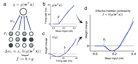
Figure 1: The effective Hebbian nonlinearity of plastic cortical networks. (a) Receptive field development between an input layer of neurons with activities $x_{i}$, connected by synaptic projections $w_{i}$ to a neuron with firing rate $y$, given by an f-I curve $y=g(\mathbf{w}^{T}\mathbf{x}))$. Synaptic connections change according to a Hebbian rule $\Delta w_{i}\propto x_{i}\ h(y)$. (b) f-I curve (blue) of a GIF model ²⁶ of a pyramidal neurons in response to step currents of 500 ms duration (dashed line: piece-wise linear fit, with slope $a=143$ Hz/nA and threshold $\theta=0.08$ nA). (c) Plasticity function of the triplet STDP model ²⁴ (blue), fitted to visual cortex plasticity data ²⁷, ²⁴, showing the weight change $\Delta w_{i}$ as a function of the post-synaptic rate $y$, under a constant pre-synaptic stimulation $x_{i}$ (dashed line: fit by quadratic function, with LTD factor $b=22.1$ Hz). (d) The combination of the f-I curve and plasticity function generates the effective Hebbian nonlinearity (dashed line: quadratic nonlinearity with LTD threshold $\theta_{1}=0.08$ nA, LTP threshold $\theta_{2}=0.23$ nA).

Sparse coding as nonlinear Hebbian learning

Beyond phenomenological modeling, normative principles that explain receptive fields development have been one of the goals of theoretical neuroscience ³¹. Sparse coding ⁶ starts from the assumptions that V1 aims at maximizing the sparseness of the activity in the sensory representation, and became a well-known normative model to develop orientation selective receptive fields ⁹, ¹², ¹³. We demonstrate that the algorithm implemented in the sparse coding model is in fact a particular example of nonlinear Hebbian learning.

The sparse coding model aims at minimizing an input reconstruction error $E=\frac{1}{2}||\mathbf{x}-\mathbf{W}\mathbf{y}||^{2}+\lambda S(\mathbf{y})$, under a sparsity constraint $S$ with relative importance $\lambda>0$. For $K$ hidden neurons $y_{j},$ such a model implicitly assumes that the vector $\mathbf{w_{j}}$ of feed-forward weights onto neuron $j$ are mirrored by hypothetical "reconstruction weights", $\mathbf{W}=[\mathbf{w}_{1}\dots\mathbf{w}_{K}]$. The resulting encoding algorithm can be recast as a neural model ³², if neurons are embedded in a feedforward model with lateral inhibition, $\mathbf{y}=g(\mathbf{w}^{T}\mathbf{x}-\mathbf{v}^{T}\mathbf{y})$, where $v$ are inhibitory recurrent synaptic connections (see Methods). In the case of a single output neuron, its firing rate is simply $y=g(\mathbf{w}^{T}\mathbf{x})$. The nonlinearity $g$ of the f-I curve is threshold-like, and determined by the choice of the sparsity constraint ³², such as the Cauchy, $L_{0}$ , or $L_{1}$ constraints (Fig 2a, see Methods).

If weights are updated through gradient descent so as to minimize $E$, the resulting plasticity rule is Oja’s learning rule ³³, $\Delta\mathbf{w}\propto\mathbf{x}\ y-\mathbf{w}\ y^{2}$. The second term $-\mathbf{w}\ y^{2}$ has a multiplicative effect on the strength of synapses projecting onto the same neuron (weight rescaling), but does not affect the receptive field shape, whereas the first term $\mathbf{x}\ y$ drives feature selectivity and receptive field formation. Together, these derivations imply that the one-unit sparse coding algorithm can be implemented by an effective nonlinear Hebbian rule combined with weight normalization. Although the plasticity mechanism is linear, $\Delta\mathbf{w}\propto\mathbf{x}\ y$, a nonlinearity arises from the f-I curve, $y=g(\mathbf{w}^{T}\mathbf{x})$, so that the effective plasticity is

$$\Delta\mathbf{w} \propto\mathbf{x}\ g(\mathbf{w}^{T}\mathbf{x})$$ (2)

This analysis reveals an equivalence between sparse coding models and neural networks with linear plasticity mechanisms, where the sparsity constraint is determined by the f-I curve $g$.

Similarly, algorithms performing independent component analysis (ICA), a model class closely related to sparse coding, also perform effective nonlinear Hebbian learning, albeit inversely, with linear neurons and a nonlinear plasticity rule ³⁴. For variants of ICA based on information maximization ⁷ or kurtosis ³⁴ different nonlinearities arise (Fig. 2a), but Eq. 2 applies equally well. Hence, various instantiations of sparse coding and ICA models not only relate to each other in their normative assumptions ³⁵, but when implemented as iterative gradient update rules, they all employ nonlinear Hebbian learning.

Simple cell development for a large class of nonlinearities

Since the models described above can be implemented by similar plasticity rules, we hypothesized nonlinear Hebbian learning to be a general principle that explains the development of receptive field selectivity. Nonlinear Hebbian learning with an effective nonlinearity $f$ is linked to an optimization principle with a function $F=\int f$ ¹⁹, ²⁰. For an input ensemble $\mathbf{x}$, optimality is achieved by weights $\tilde{\mathbf{w}}$ that maximize $\langle F(\tilde{\mathbf{w}}{}^{T}\mathbf{x})\rangle$, where angular brackets denote the average over the input statistics. Nonlinear Hebbian learning is a stochastic gradient ascent implementation of this optimization process, called projection pursuit ¹⁸, ¹⁹, ²⁰:

$$\tilde{\mathbf{w}}=max_{\mathbf{w}}\langle F(\mathbf{w}^{T}\mathbf{x})\rangle\implies\Delta\mathbf{w}\propto\mathbf{x}\ f(\mathbf{w}^{T}\mathbf{x})$$ (3)

Motivated by results from ICA theory ³⁶ and statistical properties of whitened natural images ⁵, we selected diverse Hebbian nonlinearities $f$ (Fig. 2a) and calculated the corresponding optimization value $\langle F(\mathbf{w}^{T}\mathbf{x})\rangle$ for different features of interest that we consider as candidate RF shapes, with a whitened ensemble of patches extracted from natural images as input (see Methods). These include a random connectivity pattern, a non-local oriented edge (as in principal components of natural images) and localized oriented edges (as in cat and monkey simple cells in the visual cortex), shown in Fig. 2b. The relative value of $\langle F(\mathbf{w}^{T}\mathbf{x})\rangle$ between one feature and another was remarkably consistent across various choices of the nonlinearity $f$, with localized orientation-selective receptive fields as maxima (Fig. 2b). Furthermore, we also searched for the maxima through gradient ascent, so as to confirm that the maxima are orientation selective (Fig. 2c, left). Our results indicate that receptive field development of simple cells is mainly governed by the statistical properties of natural images, while robust to specific model assumptions.

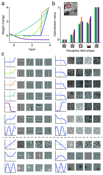
Figure 2: Simple cell development from natural images regardless of specific effective Hebbian nonlinearity. (a) Effective nonlinearity of five common models (arbitrary units): quadratic rectifier (green, as in cortical and BCM models, $\theta_{1}=1.$, $\theta_{2}=2.$), linear rectifier (dark blue, as in $L_{1}$ sparse coding or networks with linear STDP, $\theta=3.$), Cauchy sparse coding nonlinearity (light blue, $\lambda=3.$), $L_{0}$ sparse coding nonlinearity (orange, $\lambda=3.$), and negative sigmoid (purple, as in ICA models). (b) Relative optimization value $\langle F(\mathbf{w}^{T}\mathbf{x})\rangle$ for each of the five models in a, for different preselected features $\mathbf{w}$, averaged over natural image patches $\mathbf{x}$. Candidate features are represented as two-dimensional receptive fields. For all models, the optimum is achieved at the localized oriented receptive field. Inset: Example of natural image and image patch (red square) used as sensory input. (c) Receptive fields learned in four trials for ten effective Hebbian functions $f$ (from top: the five functions considered above, $u^{3}$, $-sin(u)$, $u$, $(|u|-2)_{+}$, $-cos(u)$) (left column), and their opposites $-f$ (right column). The first seven functions (above the dashed line) lead to localized oriented filters, while a sign-flip leads to random patterns. Linear or symmetric functions are exceptions and do not develop oriented filters (bottom rows).

The relevant property of natural image statistics is that the distribution of a feature derived from typical localized oriented patterns has high kurtosis ⁵, ⁶, ³⁷. Thus to establish a quantitative measure whether a nonlinearity is suitable for feature learning, we define a selectivity index (SI), which measures the relative value of $\langle F(.)\rangle$ between a variable $l$ with a Laplacian distribution and a variable $g$ with Gaussian distribution ³⁶: $SI=(\langle F(l)\rangle-\langle F(g)\rangle)/\sigma_{F}$ (see Methods). The Laplacian variable has higher kurtosis than the Gaussian variable, serving as a prototype of a kurtotic distribution. Since values obtained by filtering natural images with localized oriented patterns have a distribution with longer tails than other patterns ⁵, as does the Laplacian variable compared to the Gaussian, positive values $SI>0$ indicate good candidate functions for learning simple cell-like receptive fields from natural images. We find that each model has an appropriate parameter range where $SI>0$ (Fig. 3). For example the quadratic rectifier nonlinearity needs an LTP threshold $\theta_{2}$ below some critical level, so as to be useful for feature learning (Fig. 3a).

A sigmoidal function with threshold at zero has negative SI, but a negative sigmoid, as used in ICA studies ⁷, has $SI>0$. More generally, whenever an effective nonlinearity $f$ is not suited for feature learning, its opposite $-f$ should be, since its $SI$ will have the opposite sign (Fig. 2c). This implies that, in general, half of the function space could be suitable for feature learning ³⁶, i.e. it finds weights $w$ such that the distribution of the feature $\mathbf{w}^{T}\mathbf{x}$ has a long tail, indicating high kurtosis ("kurtotic feature"). The other half of the function space learns the least kurtotic features (e.g. random connectivity patterns for natural images, Fig. 2b,c).

This universality strongly constrains the possible shape of receptive fields that may arise during development for a given input dataset. For whitened natural images, a learnable receptive field is in general either a localized edge detector or a non-localized random connectivity pattern.

An important special case is an effective linear curve, $f(u)=u$, which arises when both f-I and plasticity curves are linear ²¹. Because the linear model maximizes variance $\langle(\mathbf{w}^{T}\mathbf{x})^{2}\rangle$, it can perform principal component analysis ³³, but does not have any feature selectivity on whitened input datasets, where variance is constant (Fig. 2c).

Symmetric effective nonlinearities, $f(u)=f(-u)$, are also exceptions, since their corresponding optimization functions are asymmetric, $F(u)=-F(-u)$, so that for datasets with symmetric statistical distributions, $P(\mathbf{x})=P(-\mathbf{x})$, the optimization value will be zero, $\langle F_{asym.}(\mathbf{w}^{T}\mathbf{x}_{sym.})\rangle=0$. As natural images are not completely symmetric, localized receptive fields do develop, though without orientation selectivity, as illustrated by a cosine function and a symmetric piece-wise linear function as effective nonlinearities (Fig. 2c, bottom rows).

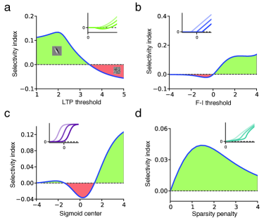
Figure 3: Selectivity index for different effective nonlinearities. (a) Quadratic rectifier (small graphic, three examples with different LTP thresholds) with LTD threshold at $\theta_{1}=1$: LTP threshold must be below $3.5$ to secure positive selectivity index (green region, main Fig) and learn localized oriented receptive fields (inset). A negative selectivity index (red region) leads to a random connectivity pattern (inset) (b) Linear rectifier: activation threshold must be above zero. (c) Sigmoid: center must be below $a=-1.2$ or, for a stronger effect, above $a=+1.2$. The opposite conditions apply to the negative sigmoid. (d) Cauchy sparse coding nonlinearity: positive but weak feature selectivity for any sparseness penalty $\lambda>0$. Insets show the nonlinearities for different choices of parameters.

Receptive field diversity

Sensory neurons display a variety of receptive field shapes ³⁸, and recent modeling efforts ⁹, ¹² have attempted to understand the properties that give rise to the specific receptive fields seen in experiments. We show here that the shape diversity of a model can be predicted by our projection pursuit analysis, and is primarily determined by the statistics of input representation, while relatively robust to the specific effective nonlinearity.

We studied a model with multiple neurons in the second layer, which compete with each other for the representation of specific features of the input. Each neuron had a piece-wise linear f-I curve and a quadratic rectifier plasticity function (see Methods) and projected inhibitory connections $v$ onto all others. These inhibitory connections are learned by anti-Hebbian plasticity and enforce decorrelation of neurons, so that receptive fields represent different positions, orientations and shapes ³⁹, ⁴⁰, ⁴¹. For 50 neurons, the resulting receptive fields became diversified (Fig. 4a-c, colored dots). In an overcomplete network of 1000 neurons, the diversity further increased (Fig. 4d-f, colored dots).

For the analysis of the simulation results, we refined our inspection of optimal oriented receptive fields for natural images by numerical evaluation of the optimality criterion $\langle F(\mathbf{w}^{T}\mathbf{x})\rangle$ for receptive fields $\mathbf{w}=\mathbf{w}_{Gabor}$, described as Gabor functions of variable length, width and spatial frequency. For all tested nonlinearities, the optimization function for single-neuron receptive fields varies smoothly with these parameters (Fig 4, grey-shaded background). The single-neuron optimality landscape was then used to analyze the multi-neuron simulation results. We found that receptive fields are located in the area where the single-neuron optimality criterion is near its maximum, but spread out so as to represent different features of the input (Fig. 4). Thus the map of optimization values, calculated from the theory of effective nonlinearity, enables us to qualitatively predict the shape diversity of receptive fields.

Although qualitatively similar, there are differences in the receptive fields developed for each model, such as smaller lengths for the $L_{0}$ sparse coding model (Fig. 4c). While potentially significant, these differences across models may be overwhelmed by differences due to other model properties, including different network sizes or input representations. This is illustrated by observing that receptive field diversity for a given model differ substantially across network sizes (Fig. 4), and the difference is even greater from simulations with an input that is not completely white (Fig. 5c). Thus our results suggests that efforts to model receptive field shapes observed experimentally ³⁸, ⁹, ¹² should focus on network size and input representation, which potentially have a stronger effect than the nonlinear properties of the specific model under consideration.

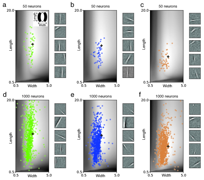
Figure 4: Optimal receptive field shapes in model networks induce diversity. (a-f) Gray level indicates the optimization value for different lengths and widths (see inset in a) of oriented receptive fields for natural images, for the quadratic rectifier (left, see Fig. 2a), linear rectifier (middle) and $L_{0}$ sparse coding (right). Optima marked with a black cross. (a-c) Colored circles indicate the receptive fields of different shapes developed in a network of 50 neurons with lateral inhibitory connections. Insets on the right show example receptive fields developed during simulation. (d-f) Same for a network of 1000 neurons.

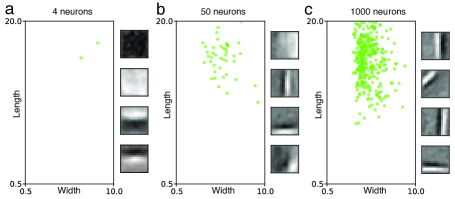
Figure 5: Receptive fields for non-whitened natural images.Images were preprocessed as in the original sparse coding study ³⁵. We simulated linear rectifier neurons ($\theta=0.5)$ with a quadratic plasticity nonlinearity ($b=0.5$). (a) Multiple-neuron simulations, with 4 neurons. The principal components dominate the optimization and receptive fields are not local, since they extend over most of the image patch. With 50 (b) and 1000 (c) neurons, lateral inhibition promotes diversity, and more localized receptive field are formed. (insets) Sample receptive fields developed for each simulation.

We also studied the variation of receptive field position and orientation. For all five nonlinearities considered, the optimization value is equal for different positions of the receptive field centers, confirming the translation invariance in the image statistics, as long as the receptive field is not too close to the border of the anatomically allowed fan-in of synaptic connections (Fig. 6b). Also, all nonlinearities reveal the same bias towards the horizontal and vertical orientations (Fig. 6c). These optimality predictions are confirmed in single neuron simulations, which lead mostly to either horizontal or vertical orientations, at random positions (Fig. 6d). When the network is expanded to 50 neurons, recurrent inhibition forces receptive fields to cover different positions, though excluding border positions, and some neurons have non-cardinal orientations (Fig. 6e). With 1000 neurons, receptive fields diversify to many possible combinations of position, orientation and length (Fig. 6f).

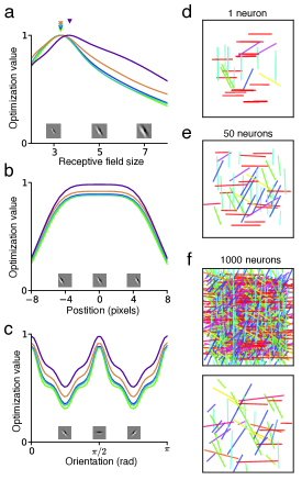
Figure 6: Diversity of receptive field size, position and orientation. (a) The optimization value of localized oriented receptive fields, within a 16x16 pixel patch of sensors, as a function of size (see Methods), for five nonlinearities (colors as in Fig. 2a). Optimal size is a receptive field of width around 3 to 4 pixels (filled triangles). (b) The optimization value as a function of position of the receptive field center, for a receptive field width of 4 pixels, indicates invariance to position within the 16x16 patch, except near the borders. (c) The optimization value as a function of orientation shows preference toward horizontal and vertical directions, for all five nonlinearities. (d) Receptive field position, orientation and length (colored bars) learned for 50 single-neuron trials. The color code indicates different orientations. (e) Receptive field positions and orientations learned in a 50 neuron network reveal diversification of positions, except at the borders. (f) With 1000 neurons, positions and orientations cover the full range of combinations (top). Selecting 50 randomly chosen receptive fields highlights the diversification of position, orientation and size (bottom). Receptive fields were learned through the quadratic rectifier nonlinearity ($\theta_{1}=1.$, $\theta_{2}=2.$).

Beyond V1 simple cells

Nonlinear Hebbian learning is not limited to explaining simple cells in V1. We investigated if the same learning principles apply to receptive field development in other visual or auditory areas or under different rearing conditions.

For auditory neurons ¹⁴, we used segments of speech as input (Fig. 7a) and observed the development of spectrotemporal receptive fields localized in both frequency and time ² (Fig. 7d). The statistical distribution of input patterns aligned with the learned receptive fields had longer tails than for random or non-local receptive fields, indicating temporal sparsity of responses (Fig. 7d). Similar to our simple cell results, the learned receptive fields show higher optimization value for all five effective nonlinearities (Fig 7g).

For a study of receptive field development in the secondary visual cortex (V2) ¹⁶, we used natural images and the standard energy model ⁴² of V1 complex cells to generate input to V2 (Fig. 7b). The learned receptive field was selective to a single orientation over neighboring positions, indicating a higher level of translation invariance. When inputs were processed with this receptive field, we found longer tails in the feature distribution than with random features or receptive fields without orientation coherence (Fig 7e), and the learned receptive field had a higher optimization value for all choices of nonlinearity (Fig 7h).

Another important constraint for developmental models are characteristic deviations, such as strabismus, caused by abnormal sensory rearing. Under normal binocular rearing conditions, the fan-in of synaptic input from the left and right eyes overlap in visual space (Fig 7c). In this case, binocular receptive fields with similar features for left and right eyes develop. In the strabismic condition, the left and right eyes are not aligned, modeled as binocular rearing with non-overlapping input from each eye (Fig. 7c). In this scenario, a monocular simple cell-like receptive field developed (Fig. 7f), as observed in experiments and earlier models ⁴³. The statistical distributions confirm that for disparate inputs the monocular receptive field is more kurtotic than a binocular one, explaining its formation in diverse models ⁴⁴ (Fig 7f,i).

Our results demonstrate the generality of the theory across multiple cortical areas. Selecting a relevant feature space for an extensive analysis, as we have done with simple cells and natural images, may not be possible in general. Nonetheless, nonlinear Hebbian learning helps to explain why some features (and not others) are learnable in network models ¹⁵.

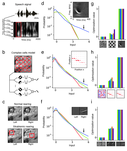
Figure 7: Nonlinear Hebbian learning across sensory modalities. (a) The auditory input is modeled as segments over time and frequency (red) of the spectrotemporal representation of speech signals. (b) The V2 input is assembled from the output of modeled V1 complex cells at different positions and orientations. Receptive fields are represented by bars with size proportional to the connection strength to the complex cell with the respective position and orientation. (c) Strabismic rearing is modeled as binocular stimuli with non-overlapping left and right eye input patches (red). (d-f) Statistical distribution (log scale) of the input projected onto three different features for speech (d), V2 (e) and strabismus (f). In all three cases, the learned receptive field (blue, inset) is characterized by a longer tailed distribution (arrows) than the random (red) and comparative (green) features. (g-i) Relative optimization value for five nonlinearities (same as in Fig. 2), for the three selected patterns (insets). The receptive fields learned with the quadratic rectifier nonlinearity ($\theta_{1}=1.$, $\theta_{2}=2.$) are the maxima among the three patterns, for all five nonlinearities, for all three datasets.

Discussion

Historically, a variety of models have been proposed to explain the development and distribution of receptive fields. We have shown that nonlinear Hebbian learning is a parsimonious principle which is implicitly or explicitly present in many developmental models ⁶, ⁷, ⁸, ⁹, ¹⁰, ¹¹, ¹², ²⁴, ³⁶, ³⁹, ⁴⁴. The fact that receptive field development is robust to the specific nonlinearity highlights a functional relation between different models. It also unifies feature learning across sensory modalities: receptive fields form around features with a long-tailed distribution.

Relation to previous studies

Earlier studies have already placed developmental models side by side, comparing their normative assumptions, algorithmic implementation or receptive fields developed. Though consistent with their findings, our results lead to revised interpretations and predictions.

The similarities between sparse coding and ICA are clear from their normative correspondence ³⁵. Nevertheless, the additional constraint in ICA, of having at most as many features as inputs, makes it an easier problem to solve, allowing for a range of suitable algorithms ³⁴. These differ from algorithms derived for sparse coding, in which the inference step is difficult due to overcompleteness. We have shown that regardless of the specific normative assumptions, it is the common implementation of nonlinear Hebbian learning that explains similarities in their learning properties.

In contrast to the idea that in sparse coding algorithms overcompleteness is required for development of localized oriented edges ³⁵, we have demonstrated that a sparse coding model with a single neuron is mathematically equivalent to nonlinear Hebbian learning and learns localized filters in a setting that is clearly "undercomplete". Thus differences observed in receptive field shapes between sparse coding and ICA models ³⁸ are likely due to differences in network size and input preprocessing. For instance, the original sparse coding model ³⁵ applied a preprocessing filter that did not completely whiten the input, leading to larger receptive fields (Fig. 5).

Studies that derive spiking models from normative theories often interpret the development of oriented receptive fields as a consequence of its normative assumptions ¹¹, ¹². In a recent example, a spiking network has been related to the sparse coding model ¹², using neural properties defined ad hoc. Our results suggest that many other choices of neural activations would have given qualitatively similar receptive fields, independent of the sparse coding assumption. While in sparse coding the effective nonlinearity derives from a linear plasticity rule combined with a nonlinear f-I curve, our results indicate that a nonlinear plasticity rule combined with a linear neuron model would give the same outcome.

In order to distinguish between different normative assumptions, or particular neural implementations, the observation of "oriented filters" is not sufficient and additional constraints are needed. Similarly receptive shape diversity, another important experimental constraint, should also be considered with care, since it cannot easily distinguish between models either. Studies that confront the receptive field diversity of a model to experimental data ⁹, ¹², ³⁸ should also take into account input preprocessing choices and how the shape changes with an increasing network size, since we have observed that these aspects may have a larger effect on receptive field shape than the particulars of the learning model.

Empirical studies of alternative datasets, including abnormal visual rearing ⁴⁴, tactile and auditory stimuli ¹⁵, have also observed that different unsupervised learning algorithms lead to comparable receptive fields shapes. Our results offer a plausible theoretical explanation for these findings.

Past investigations on nonlinear Hebbian learning ²⁰, ³⁶ demonstrated that many nonlinearities were capable of solving the cocktail party problem. Since it is a specific toy model, that asks for the unmixing of linearly mixed independent features, it is not clear a priori whether the same conclusions would hold in other settings. We have shown that the results of Fyfe and Baddeley ²⁰ and Hyvarinen and Oja ³⁶ generalize in two directions. First, the effective nonlinear Hebbian learning mechanism is also behind other models beyond ICA, such as sparse coding models and plastic spiking networks. Second, the robustness to the choice of nonlinearity is not limited to a toy example, but also holds in multiple real world data. Together, these insights explain and predict the outcome of many developmental models, in diverse applications.

Robustness to normative assumptions

Many theoretical studies start from normative assumptions ⁷, ⁹, ¹¹, ³⁵, such as a statistical model of the sensory input or a functional objective, and derive neural and synaptic dynamics from them. Our claim of universality of feature learning indicates that details of normative assumptions may be of lower importance.

For instance, in sparse coding one assumes features with a specific statistical prior ⁹, ³⁵. After learning, this prior is expected to match the posterior distribution of the neuron’s firing activity ⁹, ³⁵. Nevertheless, we have shown that receptive field learning is largely unaffected by the choice of prior. Thus, one cannot claim that the features were learned because they match the assumed prior distribution, and indeed in general they do not. For a coherent statistical interpretation, one could search for a prior that would match the feature statistics. However, since the outcome of learning is largely unaffected by the choice of prior, such a statistical approach would have limited predictive power. Generally, kurtotic prior assumptions enable feature learning, but the specific priors are not as decisive as one might expect. Because normative approaches have assumptions, such as independence of hidden features, that are not generally satisfied by the data they are applied to, the actual algorithm that is used for optimization becomes more critical than the formal statistical model.

The concept of sparseness of neural activity is used with two distinct meanings. The first one is a single-neuron concept and specifically refers to the long-tailed distribution statistics of neural activity, indicating a "kurtotic" distribution. The second notion of sparseness is an ensemble concept and refers to the very low firing rate of neurons, observed in cortical activity ⁴⁵, which may arise from lateral competition in overcomplete representations. Overcompleteness of ensembles makes sparse coding different from ICA ³⁵. We have shown here that competition between multiple neurons is fundamental for receptive field diversity, whereas it is not required for simple cell formation per se. Kurtotic features can be learned even by a single neuron with nonlinear Hebbian learning, and with no restrictions on the sparseness of its firing activity.

Interaction of selectivity with preprocessing and homeostasis

The concept of nonlinear Hebbian learning also clarifies the interaction of feature selectivity with preprocessing mechanisms. We have assumed whitened data throughout the study, except Fig. 5. Since after whitening second-order correlations are uninformative, neurons can develop sensitivity to higher order features. While whitened data is formally not required for our analysis, second-order correlations may dominate the optimization for non-white input, so that principal components will be learned (Fig. 5a). Only when multiple neurons are added and receptive fields diversify, are localized simple cells formed with an input that is not completely white ³⁵ (Fig. 5c).

In studies of spiking networks, the input is restricted to positive rates, possibly through an on/off representation, as observed in the LGN ⁴⁶. While the center-surround properties of LGN contributes to a partial decorrelation of neuronal activity ⁴⁷, in such alternative representations, trivial receptive fields may develop, such as a single non-zero synapse, and additional mechanisms, such as hard bounds on each synaptic strength, $a\leq w_{j}\leq b$, may be necessary to restrict the optimization space to desirable features ¹⁰.

Instead of constraining the synaptic weights, one may implement a synaptic decay as in Oja’s plasticity rule ³³, $\Delta w\propto x\cdot y-w\cdot y^{2}$ (see also ⁴⁸). Because of its multiplicative effect, the decay term does not alter the receptive field, but only scales its strength. Thus, it is equivalent to rescaling the input in the f-I curve, so as to shift it to the appropriate range (Fig. 3). Similar scaling effects arise from f-I changes due to intrinsic plasticity ¹¹, ²⁸, ⁴⁹. The precise relation between nonlinear Hebbian learning, spiking representations and homeostasis in the cortex is an important topic for further studies.

Universality supports biological instantiation

The principle of nonlinear Hebbian learning has a direct correspondence to biological neurons and is compatible with a large variety of plasticity mechanisms. It is not uncommon for biological systems to have diverse implementations with comparable functional properties ⁵⁰. Different species, or brain areas, could have different neural and plasticity characteristics, and still have similar feature learning properties ⁵¹, ⁵². The generality of the results discussed in this paper reveals learning simple cell-like receptive fields from natural images to be much easier than previously thought. It implies that a biological interpretation of models is possible even if some aspects of a model appear simplified or even wrong in some biological aspects. Universality also implies that the study of receptive field development is not sufficient to distinguish between different models.

The relation of nonlinear Hebbian learning to projection pursuit endorses the interpretation of cortical plasticity as an optimization process. Under the rate coding assumptions considered here, the crucial property is an effective synaptic change linear in the pre-synaptic rate, and nonlinear in the post-synaptic input. Pairing experiments with random firing and independently varying pre- and post-synaptic rates would be valuable to investigate these properties ²⁷, ⁵³, ⁵⁴. Altogether, the robustness to details in both input modality and neural implementation suggests nonlinear Hebbian learning as a fundamental principle underlying the development of sensory representations.

Methods

Spiking model. A generalized leaky integrate-and-fire neuron ²⁶ was used as spiking model, which includes power-law spike-triggered adaptation and stochastic firing, with parameters ²⁶ fitted to pyramidal neurons. The f-I curve $g(I)$ was estimated by injecting step currents and calculating the trial average of the spike count over the first $500$ ms. The minimal triplet-STDP model²⁴ was implemented, in which synaptic changes follow

$$\frac{d}{dt}w(t)=A^{+}y(t)\bar{y}^{+}(t)\bar{x}^{+}(t)-A^{-}x(t)\bar{y}^{-}(t)$$ (4)

where $y(t)$ and $x(t)$ are the post- and pre-synaptic spike trains, respectively: $y(t)=\sum_{f}\delta(t-t^{f})$, where $t^{f}$ are the firing times and $\delta$ denotes the Dirac $\delta$-function; $x(t)$ is a vector with components $x_{i}(t)=\sum_{f}\delta(t-t_{i}^{f})$, where $t_{i}^{f}$ are the firing times of pre-synaptic neuron $i$; $w$ is a vector comprising the synaptic weights $w_{i}$ connecting a pre-synaptic neuron $i$ to a post-synaptic cell. $A^{+}=6.5\cdot 10^{-3}$ and $A^{-}=5.3\cdot 10^{-3}$ are constants, and $\bar{y}^{+}$, $\bar{x}^{+}$ and $\bar{y}^{-}$ are moving averages, implemented by integration (e.g. $\tau\frac{\partial\bar{{y}}}{\partial t}=-\bar{y}+y$), with time scales $114.0$ ms, $16.8$ ms and $33.7$ ms, respectively ²⁴. For estimating the nonlinearity $h(y)$ of the plasticity, pre- and post-synaptic spike trains were generated as Poisson processes, with the pre-synaptic rate set to $20$ Hz.

A linear rectifier $g(x)=a(x-b)_{+}$ was fitted to the f-I curve of the spiking neuron model by squared error optimization. Similarly, a quadratic function $h(x)=a(x^{2}-bx)$ was fitted to the nonlinearity of the triplet STDP model. The combination of these two fitted functions was plotted as fit for the effective nonlinearity $f(x)=h(g(x))$.

Sparse coding analysis. A sparse coding model, with $K$ neurons $y_{1},\dots,y_{K}$, has a nonlinear Hebbian learning formulation. The sparse coding model minimizes a least square reconstruction error between the vector of inputs $\mathbf{x}$ and the reconstruction vector $\mathbf{W}\mathbf{y},$ where $\mathbf{W}=[\mathbf{w}_{1}\dots\mathbf{w}_{K}]$, and $\mathbf{y}=(y_{1},\dots,y_{K})$ is the vector of neuronal activities, with $y_{j}\geq 0$ for $1\leq j\leq K$. The total error $E$ combines a sparsity constraint $S$ with weight $\lambda$ and the reconstruction error, $E=\frac{1}{2}||\mathbf{x}-\mathbf{W}\mathbf{y}||^{2}+\lambda\sum S(y_{k})$. $E$ has to be minimal, averaged across all input samples, under the constraint $y_{j}\geq 0$ for all $j$.

The minimization problem is solved by a two-step procedure. In the first step, for each input sample, one minimizes $E$ with respect to all hidden units $y_{j}$

$$\frac{d}{dy_{j}}E=0 \iff\mathbf{w}_{j}(\mathbf{x}-\mathbf{W}\mathbf{y})-\lambda S^{\prime}(y_{j})=0$$ (5)

$$\iff\mathbf{w}_{j}\mathbf{x}-\sum_{k\neq j}(\mathbf{w}_{j}^{T}\mathbf{w}_{k})y_{k}-||\mathbf{w}_{j}||^{2}y_{j}-\lambda S^{\prime}(y_{j})=0$$

$$\iff y_{j}+\lambda S^{\prime}(y_{j})=\mathbf{w}_{j}^{T}\mathbf{x}-\sum_{k\neq j}(\mathbf{w}_{j}^{T}\mathbf{w}_{k})y_{k}$$

$$\iff y_{j}=g(\mathbf{w}_{j}^{T}\mathbf{x}-\sum_{k\neq j}v_{jk}y_{k})$$

where we constrained the vector $\mathbf{w}_{j}$ of synapses projecting onto unit $y_{j}$ by $||\mathbf{w}_{j}||^{2}=1$, defined the activation function $g(.)=T^{-1}(.)$, the inverse of $T(y)=(y+\lambda S^{\prime}(y))$, and defined recurrent synaptic weights $v_{jk}=\mathbf{w}_{j}^{T}\mathbf{w}_{k}$. For each input sample $\mathbf{x}$, this equation shall be iterated until convergence. The equation can be interpreted as a recurrent neural network, where each neuron has an activation function $g$, and the input is given by the sum of the feedforward drive $\mathbf{w}_{j}^{T}\mathbf{x}$ and a recurrent inhibition term $-\sum_{k\neq j}v_{jk}y_{k}$. To avoid instability, we implement a smooth membrane potential $u_{j}$, which has the same convergence point ³²

$$\tau_{u}\frac{d}{dt}u_{j}(t)=-u_{j}(t)+(\mathbf{w}_{j}^{T}\mathbf{x}-\sum_{k\neq j}v_{jk}y_{k}(t))$$ (6)

$$y_{j}(t)=g(u_{j}(t))$$

initialized with $u_{j}(t)=0$.

The second step is a standard gradient descent implementation of the least square regression optimization, leading to an learning rule

$$\Delta w_{j}\propto\frac{d}{dw_{j}}E=(\mathbf{x}-\mathbf{W}^{T}\mathbf{y})\ y_{j}=\mathbf{x}\ y_{j}-\mathbf{w}_{j}\ y_{j}^{2}-\sum_{k\neq j}\mathbf{w}_{k}y_{k}y_{j}$$

The decay term $\mathbf{w}_{j}\ y_{j}^{2}$ has no effect, since the norm is constrained to $||\mathbf{w}_{j}||=1$ at each step. For a single unit $y,$ the model simplifies to a nonlinear Hebbian formulation, $\Delta\mathbf{w}\propto\mathbf{x}\ g(\mathbf{w}_{j}^{T}\mathbf{x})$. For multiple units, it can be interpreted as projection pursuit on an effective input, not yet represented by other neurons, $\tilde{\mathbf{x}_{j}}=\mathbf{x}-\sum_{k\neq j}\mathbf{w}_{k}y_{k}$, which simplifies to $\Delta\mathbf{w}_{j}\propto\tilde{\mathbf{x}}_{j}\cdot g(\mathbf{w}_{j}^{T}\tilde{\mathbf{x}_{j}})$ .

There are two non-local terms that need to be implemented by local mechanisms so as to be biologically plausible. First, the recurrent weights depend on the overlap between receptive fields, $\mathbf{w}_{j}^{T}\mathbf{w}_{k}$, which is non-local. The sparse coding model assumes independent hidden neurons, which implies that after learning neurons should be pair-wise uncorrelated, $cov(y_{j},y_{k})=0$. As an aside we note that the choice $v_{jk}=\mathbf{w}_{j}^{T}\mathbf{w}_{k}$ does not automatically guarantee decorrelation. Decorrelation may be enforced through plastic lateral connections, following an anti-Hebbian rule ³⁹, ¹², $\Delta v_{jk}\propto(y_{j}-\langle y_{j}\rangle)\cdot y_{k}$, where $\langle y_{j}\rangle$ is a moving average (we use $\tau=1000$ input samples). Thus by substituting fixed recurrent connections by anti-Hebbian plasticity, convergence $\Delta v_{jk}=0$ implies $cov(y_{j},y_{k})=0$. While this implementation does not guarantee $v_{jk}=\mathbf{w}_{j}^{T}\mathbf{w}_{k}$ after convergence, neither does $v_{jk}=\mathbf{w}_{j}^{T}\mathbf{w}_{k}$ guarantee decorrelation $cov(y_{j},y_{k})=0$, it does lead to optimal decorrelation, which is the basis of the normative assumption. Additionally we constrain $v_{jk}\geq 0$ to satisfy Dale’s law. Although some weights would converge to negative values otherwise, most neuron pairs have correlated receptive fields, and thus positive recurrent weights.

Second, we ignore the non-local term $\sum_{k\neq j}\mathbf{w}_{k}y_{k}y_{j}$ in the update rule. Although this approximation is not theoretically justified, we observed in simulations that receptive fields do not qualitatively differ when this term is removed.

The resulting Hebbian formulation can be summarized as

$$y_{j}=g(\mathbf{w}_{j}^{T}\mathbf{x}-\sum_{k\neq j}v_{jk}y_{k})$$ (7)

$$\Delta\mathbf{w}_{j}\propto\mathbf{x\ }y_{j}$$

$$\Delta v_{jk}\propto(y_{j}-\langle y_{j}\rangle)\cdot y_{k}$$

This derivation unifies previous results on the biological implementation of sparse coding: the relation of the sparseness constraint to a specific activation function ³², the derivation of a Hebbian learning rule from quadratic error minimization ³³, and the possibility of approximating lateral interaction terms by learned lateral inhibition ³⁹, ¹².

Nonlinearities and optimization value. The optimization value for a given effective nonlinearity $f$, synaptic weights $w$, and input samples $x$, is given by $R=\langle F(\mathbf{w}^{T}\mathbf{x})\rangle$, where $F=\int f$ and angular brackets indicate the ensemble average over $x$. Relative optimization values in Figs. 2b and 6 were normalized to $[0,1]$, relative to the minimum and maximum values among the considered choice of features $w$, $R^{*}=(R-R_{min})/(R_{max}-R_{min})$. The selectivity index of a nonlinearity $f$ is defined as $SI=(\langle F(l)\rangle-\langle F(g)\rangle)/\sigma_{F}$, where $l$ and $g$ are Laplacian and Gaussian variables respectively, normalized to unit variance. $\sigma_{F}=\sqrt{\sigma_{F(l)}\sigma_{F(g)}}$ is a normalization factor, with $\sigma_{F(.)}=\sqrt{\langle F(.)^{2}\rangle}$. The selectivity of an effective nonlinearity $f$ is not altered by multiplicative scaling, $\tilde{f}(u)=\alpha f(u)$, neither by additive constants when the input distribution is symmetric, $\tilde{f}(u)=\alpha f(u)+\beta$. The effective nonlinearities in Fig. 2 included the linear rectifier $f(u)=\begin{cases}0,&if\ u<\theta\\ u-\theta,&if\ u\geq\theta\end{cases}$, the quadratic rectifier $f(u)=\begin{cases}0,&if\ u<\theta\\ (u-\theta)(u-\theta-b),&if\ u\geq\theta\end{cases}$, the $L_{0}$ sparse coding nonlinearity $f(u)=\begin{cases}0,&if\ u<\lambda\\ u,&if\ u\geq\lambda\end{cases}$, the Cauchy sparse coding nonlinearity $f=T^{-1}$, where $T(y)=\begin{cases}0,&if\ y<0\\ y+2\lambda y/(1+y^{2}),&if\ y\geq 0\end{cases}$, the negative sigmoid $f(u)=1-2/(1+e^{-2u})$, a polynomial function $f(u)=u^{3}$, trigonometric functions $sin(u)$ and $cos(u)$, a symmetric piece-wise linear function $f(u)=\begin{cases}0,&if\ |u|<\theta\\ |u|-\theta,&if\ |u|\geq\theta\end{cases}$, as well as, for comparison, a linear function $f(u)=u$.

Receptive field learning. Natural image patches (16 by 16 pixel windows) were sampled from a standard dataset ⁶ ($10^{6}$ patches). Patches were randomly rotated by $\pm 90{}^{\circ}$ degrees to avoid biases in orientation. The dataset was whitened by mean subtraction and a standard linear transformation $\mathbf{x}^{*}=\mathbf{M}\mathbf{x}$, where $\mathbf{M}=\mathbf{R}\mathbf{D}^{-1/2}\mathbf{R}^{T}$ and $\langle\mathbf{x}\mathbf{x}^{T}\rangle=\mathbf{R}\mathbf{D}\mathbf{R}^{T}$ is the eigenvalue decomposition of the input correlation matrix. In Fig. 5, we used images preprocessed as in Olshausen and Field ⁶, filtered in the spatial frequency domain by $M(f)=f\ e^{-(f/f_{0})^{4}}$. The exponential factor is a low-pass filter that attenuates high-frequency spatial noise, with $f_{0}=200$ cycles per image. The linear factor $f$ was designed to whiten the images by canceling the approximately $1/f$ power law spatial correlation observed in natural images ³⁷. But since the exponent of the power law for this particular dataset has an exponent closer to $1.2$, the preprocessed image exhibit higher variance at lower spatial frequencies.

Synaptic weights were initialized randomly (normal distribution with zero mean) and, for an effective nonlinearity $f$, evolved through $\mathbf{w}_{k+1}=\mathbf{w}_{k}+\eta\ \mathbf{x}\ f(\mathbf{w}_{k}^{T}\mathbf{x}_{k})$, for each input sample $x_{k}$, with a small learning rate $\eta$. We enforced normalized weights at each time step, $||\mathbf{w}||_{2}=1$, through multiplicative normalization, implicitly assuming rapid homeostatic mechanisms ²⁸, ⁵⁵. For multiple neurons, the neural version of the sparse coding model described in Eq 7 was implemented. In Fig 4 and 5, the learned receptive fields were fitted to Gabor filters by least square optimization. Receptive fields with less than $0.6$ variance explained were rejected (less than 5% of all receptive fields).

Receptive field selection. In Fig. 2b, the five selected candidate patterns are: random connectivity filter (weights sampled independently from the normal distribution with zero mean), high-frequency Fourier filter (with equal horizontal and vertical spatial periods, $T_{x}=T_{y}=8$ pixels), difference of Gaussians filter ($\sigma_{1}=3.$, $\sigma_{2}=4.$), low-frequency Fourier filter ($T_{x}=16$, $T_{y}=32$), and centered localized Gabor filter ($\sigma_{x}=1.5$, $\sigma_{y}=2.0$, $f=0.2$, $\theta=\pi/3$, $\phi=\pi/2$). Fourier filters were modeled as $w_{ab}=sin(2\pi a/T_{x})*cos(2\pi b/T_{y})$; difference of Gaussians filters as the difference between two centered 2D Gaussians with same amplitude and standard deviations $\sigma_{1}$ and $\sigma_{2}$; and we considered standard Gabor filters, with center $(x_{c},y_{c}),$ spatial frequency $f$, width $\sigma_{x}$, length $\sigma_{y},$ phase $\phi$ and angle $\theta$. In Fig 4 and 5 we define the Gabor width and length in pixels as 2.5 times the standard deviation of the respective Gaussian envelopes, $\sigma_{x}$ and $\sigma_{y}$. In Fig. 6a, a Gabor filter of size $s$ had parameters $\sigma_{x}=0.3\cdot s$, $\sigma_{y}=0.6\cdot s$, $f=1/s$ and $\theta=\pi/3$. In Fig. 6b-c, the Gabor filter parameters were $\sigma_{x}=1.2$, $\sigma_{y}=2.4$, $f=0.25$. All receptive fields were normalized to $||\mathbf{w}||_{2}=1$. In Fig. 4 and 5, the background optimization value was calculated for Gabor filters of different widths, lengths, frequencies, phases $\phi=0$ and $\phi=\pi/2$. For each width and length, the maximum value among frequencies and phases was plotted.

Additional datasets. For the strabismus model, two independent natural image patches were concatenated, representing non-overlapping left and right eye inputs, forming a dataset with 16 by 32 patches ⁴³. For the binocular receptive field in the strabismus statistical analysis (Fig. 7a), a receptive field was learned with a binocular input with same input from left and right eyes. As V2 input, V1 complex cell responses were obtained from natural images as in standard energy models ⁴², modeled as the sum of the squared responses of simple cells with alternated phases. These simple cells were modeled as linear neurons with Gabor receptive fields ($\sigma_{x}=1.2$, $\sigma_{y}=2.4$, $f=0.3$), with centers placed on a 8 by 8 grid (3.1 pixels spacing), with 8 different orientations at each position (total of 512 input dimensions). For the non-orientation selective receptive field in the V2 statistical analysis (Fig. 7d), the orientations of the input complex cells for the learned receptive field were randomized. As auditory input, spectrotemporal segments were sampled from utterances spoken by a US English male speaker (CMU US BDL ARCTIC database, Kominek and Black ⁵⁶). For the frequency decomposition ¹⁴, each audio segment was filtered by gammatone kernels, absolute and log value taken and downsampled to $50$ Hz. Each sample was 20 time points long ($400$ ms segment) and 20 frequency points wide (equally spaced between $0.2$ kHz and $4.0$ kHz). For the non-local receptive field in the auditory statistical analysis (Fig. 7g), a Fourier filter was used ($T_{t}=T_{f}=10$). For all datasets, the input ensemble was whitened after the preprocessing steps, by the same linear transformation described above for natural images, and all receptive fields were normalized to $||\mathbf{w}||_{2}=1$.

References

- Hubel and Wiesel 1959 David H. Hubel and Torsten N. Wiesel. Receptive fields of single neurones in the cat’s striate cortex. The Journal of physiology, 148(3):574, 1959.
- Miller et al. 2002 Lee M. Miller, Monty A. Escabi, Heather L. Read, and Christoph E. Schreiner. Spectrotemporal receptive fields in the lemniscal auditory thalamus and cortex. Journal of neurophysiology, 87(1):516–527, 2002.
- DiCarlo et al. 2012 James J. DiCarlo, Davide Zoccolan, and Nicole C. Rust. How does the brain solve visual object recognition? Neuron, 73(3):415–434, 2012.
- Freeman and Simoncelli 2011 Jeremy Freeman and Eero P Simoncelli. Metamers of the ventral stream. Nat Neurosci, 14(9):1195–1201, 2011.
- Field 1994 David Field. What is the goal of sensory coding? Neural computation, 6(4):559–601, 1994.
- Olshausen and Field 1996 Bruno A. Olshausen and David J. Field. Emergence of simple-cell receptive field properties by learning a sparse code for natural images. Nature, 381(6583):607–609, 1996.
- Bell and Sejnowski 1997 Anthony J. Bell and Terrence J. Sejnowski. The “independent components” of natural scenes are edge filters. Vision Research, 37(23):3327–3338, 1997.
- Law and Cooper 1994 C C Law and L N Cooper. Formation of receptive fields in realistic visual environments according to the bienenstock, cooper, and munro (BCM) theory. Proceedings of the National Academy of Sciences, 91(16):7797–7801, 1994.
- Rehn and Sommer 2007 M. Rehn and F. T Sommer. A network that uses few active neurones to code visual input predicts the diverse shapes of cortical receptive fields. Journal of Computational Neuroscience, 22(2):135–146, 2007.
- Clopath et al. 2010 C. Clopath, L. Busing, E. Vasilaki, and W. Gerstner. Connectivity reflects coding: a model of voltage-based STDP with homeostasis. Nature Neuroscience, 13(3):344–352, 2010.
- Savin et al. 2010 Cristina Savin, Prashant Joshi, and Jochen Triesch. Independent component analysis in spiking neurons. PLoS computational biology, 6(4):e1000757, 2010.
- Zylberberg et al. 2011 Joel Zylberberg, Jason Timothy Murphy, and Michael Robert DeWeese. A sparse coding model with synaptically local plasticity and spiking neurons can account for the diverse shapes of v1 simple cell receptive fields. PLoS Comput Biol, 7(10):e1002250, 2011.
- Olshausen and Field 2004 Bruno A Olshausen and David J Field. Sparse coding of sensory inputs. Current Opinion in Neurobiology, 14(4):481–487, 2004.
- Smith and Lewicki 2006 Evan C. Smith and Michael S. Lewicki. Efficient auditory coding. Nature, 439(7079):978–982, 2006.
- Saxe et al. 2011 Andrew Saxe, Maneesh Bhand, Ritvik Mudur, Bipin Suresh, and Andrew Y. Ng. Unsupervised learning models of primary cortical receptive fields and receptive field plasticity. Advances in neural information processing systems, pages 1971–1979, 2011.
- Lee et al. 2007 H. Lee, C. Ekanadham, and A. Ng. Sparse deep belief net model for visual area v2. Advances in neural information processing systems, 20, 2007.
- Yamins et al. 2014 Daniel LK Yamins, Ha Hong, Charles F. Cadieu, Ethan A. Solomon, Darren Seibert, and James J. DiCarlo. Performance-optimized hierarchical models predict neural responses in higher visual cortex. Proceedings of the National Academy of Sciences, 111(23):8619–8624, 2014.
- Friedman 1987 Jerome H. Friedman. Exploratory projection pursuit. Journal of the American Statistical Association, 82(397):249–66, 1987.
- Oja et al. 1991 E. Oja, H. Ogawa, and J. Wangviwattana. Learning in nonlinear constrained hebbian networks. Artificial Neural Networks, 1991.
- Fyfe and Baddeley 1995 Colin Fyfe and Roland Baddeley. Non-linear data structure extraction using simple hebbian networks. Biological Cybernetics, 72(6):533–541, 1995.
- Miller et al. 1989 K. D. Miller, J. B. Keller, and M. P. Stryker. Ocular dominance column development: analysis and simulation. Science, 245(4918):605–615, 1989.
- Bienenstock et al. 1982 E. L. Bienenstock, L. N. Cooper, and P. W. Munro. Theory for the development of neuron selectivity: orientation specificity and binocular interaction in visual cortex. The Journal of Neuroscience, 2(1):32–48, 1982.
- Gerstner et al. 2014 Wulfram Gerstner, Werner M. Kistler, Richard Naud, and Liam Paninski. Neuronal Dynamics: From Single Neurons to Networks and Models of Cognition. Cambridge University Press, 2014.
- Pfister and Gerstner 2006 J. P Pfister and W. Gerstner. Triplets of spikes in a model of spike timing-dependent plasticity. The Journal of Neuroscience, 26(38):9673–9682, 2006.
- Wiesel and Hubel 1963 Torsten N. Wiesel and David H. Hubel. Single-cell responses in striate cortex of kittens deprived of vision in one eye. J Neurophysiol, 26(6):1003–1017, 1963.
- Pozzorini et al. 2013 Christian Pozzorini, Richard Naud, Skander Mensi, and Wulfram Gerstner. Temporal whitening by power-law adaptation in neocortical neurons. Nature Neuroscience, 16(7):942–948, 2013.
- Sjostrom et al. 2001 P. J Sjostrom, G. G Turrigiano, and S. B Nelson. Rate, timing, and cooperativity jointly determine cortical synaptic plasticity. Neuron, 32(6):1149–1164, 2001.
- Turrigiano 2011 G. Turrigiano. Too many cooks? intrinsic and synaptic homeostatic mechanisms in cortical circuit refinement. Annual review of neuroscience, 34:89–103, 2011.
- Song et al. 2000 S. Song, K. D Miller, and L. F Abbott. Competitive hebbian learning through spike-timing-dependent synaptic plasticity. Nature Neuroscience, 3(9):919–926, 2000.
- Gerstner et al. 1996 W. Gerstner, R. Kempter, and J. L Van Hemmen. A neuronal learning rule for sub-millisecond temporal coding. Nature, 383(6595):76–78, 1996.
- Dayan and Abbott 2001 P. Dayan and L. F. Abbott. Theoretical neuroscience, volume 31. MIT press Cambridge, MA, 2001.
- Rozell et al. 2008 Christopher J. Rozell, Don H. Johnson, Richard G. Baraniuk, and Bruno A. Olshausen. Sparse coding via thresholding and local competition in neural circuits. Neural Computation, 20(10):2526–2563, 2008.
- Oja 1982 Erkki Oja. Simplified neuron model as a principal component analyzer. Journal of mathematical biology, 15(3):267–273, 1982.
- Hyvarinen and Oja 2000 A. Hyvarinen and E. Oja. Independent component analysis: algorithms and applications. Neural networks, 13(4-5):411–430, 2000.
- Olshausen and Field 1997 B. A Olshausen and D. J Field. Sparse coding with an overcomplete basis set: A strategy employed by v1? Vision research, 37(23):3311–3325, 1997.
- Hyvarinen and Oja 1998 Aapo Hyvarinen and Erkki Oja. Independent component analysis by general nonlinear hebbian-like learning rules. Signal Processing, 64(3):301–313, 1998.
- Ruderman and Bialek 1994 Daniel L. Ruderman and William Bialek. Statistics of natural images: Scaling in the woods. Physical Review Letters, 73(6):814–817, 1994.
- Ringach 2002 Dario L. Ringach. Spatial structure and symmetry of simple-cell receptive fields in macaque primary visual cortex. Journal of Neurophysiology, 88(1):455–463, 2002.
- Foldiak 1990 P. Foldiak. Forming sparse representations by local anti-hebbian learning. Biological cybernetics, 64(2):165–170, 1990.
- Vogels et al. 2011 T. P. Vogels, Henning Sprekeler, Friedemann Zenke, Claudia Clopath, and Wulfram Gerstner. Inhibitory plasticity balances excitation and inhibition in sensory pathways and memory networks. Science, 334(6062):1569–1573, 2011.
- King et al. 2013 Paul D. King, Joel Zylberberg, and Michael R. DeWeese. Inhibitory interneurons decorrelate excitatory cells to drive sparse code formation in a spiking model of v1. The Journal of Neuroscience, 33(13):5475–5485, 2013.
- Hyvarinen et al. 2009 A. Hyvarinen, J. Hurri, and P. O. Hoyer. Natural Image Statistics: A Probabilistic Approach to Early Computational Vision., volume 39. Springer, 2009.
- Cooper et al. 2004 Leon N. Cooper, Nathan Intrator, Brian S. Blais, and Harel Z. Shouval. Theory of Cortical Plasticity. World Scientific Pub Co Inc, 2004.
- Hunt et al. 2013 Jonathan J. Hunt, Peter Dayan, and Geoffrey J. Goodhill. Sparse coding can predict primary visual cortex receptive field changes induced by abnormal visual input. PLoS Comput Biol, 9(5):e1003005, 2013.
- Barth and Poulet 2012 Alison L. Barth and James F.A. Poulet. Experimental evidence for sparse firing in the neocortex. Trends in Neurosciences, 35(6):345–355, 2012.
- Miller 1994 Kenneth D. Miller. A model for the development of simple cell receptive fields and the ordered arrangement of orientation columns through activity-dependent competition between on-and off-center inputs. Journal of Neuroscience, 14:409–409, 1994.
- Dan et al. 1996 Yang Dan, Joseph J. Atick, and R. Clay Reid. Efficient coding of natural scenes in the lateral geniculate nucleus: Experimental test of a computational theory. The Journal of Neuroscience, 16(10):3351–3362, 1996.
- Chen et al. 2013 Jen-Yung Chen, Peter Lonjers, Christopher Lee, Marina Chistiakova, Maxim Volgushev, and Maxim Bazhenov. Heterosynaptic plasticity prevents runaway synaptic dynamics. The Journal of Neuroscience, 33(40):15915–15929, 2013.
- Elliott 2014 Terry Elliott. Sparseness, antisparseness and anything in between: The operating point of a neuron determines its computational repertoire. Neural computation, pages 1–49, 2014.
- Prinz et al. 2004 Astrid A. Prinz, Dirk Bucher, and Eve Marder. Similar network activity from disparate circuit parameters. Nature Neuroscience, 7(12):1345–1352, 2004.
- Sharma et al. 2000 Jitendra Sharma, Alessandra Angelucci, and Mriganka Sur. Induction of visual orientation modules in auditory cortex. Nature, 404(6780):841–847, 2000.
- Kaschube et al. 2010 Matthias Kaschube, Michael Schnabel, Siegrid Lowel, David M. Coppola, Leonard E. White, and Fred Wolf. Universality in the evolution of orientation columns in the visual cortex. Science, 330(6007):1113–1116, 2010.
- Sjostrom et al. 2008 P. Jesper Sjostrom, Ede A. Rancz, Arnd Roth, and Michael Hausser. Dendritic excitability and synaptic plasticity. Physiol. Rev., 88(2):769–840, 2008.
- Graupner and Brunel 2012 Michael Graupner and Nicolas Brunel. Calcium-based plasticity model explains sensitivity of synaptic changes to spike pattern, rate, and dendritic location. Proceedings of the National Academy of Sciences, 109(10):3991–3996, 2012.
- Zenke et al. 2013 Friedemann Zenke, Guillaume Hennequin, and Wulfram Gerstner. Synaptic plasticity in neural networks needs homeostasis with a fast rate detector. PLoS computational biology, 9(11):e1003330, 2013.
- Kominek and Black 2004 John Kominek and Alan W. Black. The CMU Arctic speech databases. 2004.