ACTIN AUTOMATA WITH MEMORY

Abstract

Actin is a globular protein which forms long polar filaments in eukaryotic. The actin filaments play roles of cytoskeleton, motility units , information processing and learning. We model actin filament as a double chain of finite state machines, nodes, which take states ‘0’ and ‘1’. The states are abstractions of absence and presence of a sub-threshold charge on an actin units corresponding to the nodes. All nodes update their state in parallel in discrete time. A node updates its current state depending on states of two closest neighbours in the node chain and two closest neighbours in the complementary chain. Previous models of actin automata considered momentary state transitions of nodes. We enrich the actin automata model by assuming that states of nodes depends not only on the current states of neighbouring node but also on their past states. Thus, we assess the effect of memory of past states on the dynamics of acting automata. We demonstrate in computational experiments that memory slows down propagation of perturbations, decrease entropy of space-time patterns generated, transforms travelling localisations to stationary oscillators, and stationary oscillations to still patterns.

1 Introduction

Actin is a globular protein presented as intracellular, cytoskeleton, filaments in eukariotic cells from unicellular organisms to plants and animals. Actin filaments, together with tubule microtubule filaments, are not only key components responsible for coordinated motility of cells but are ‘nervous system’ of the cells. The actin and tubule filaments process information and implement learning Hameroff [1988]; Rasmussen et al. [1990]; Ludin & Matus [1993]; Conrad [1996]; Tuszynski et al. [1998]; Priel et al. [2006]; Debanne [2004]; Priel et al. [2010]; Jaeken [2007]. Disfunction in actin assembly or the actin association with other intracellular components leads to psychiatric and neurological disorders Van Woerkom [1990]; Fiala et al. [2002]; Persico & Bourgeron [2006]; Sekino et al. [2007]; van Spronsen & Hoogenraad [2010]; Kojima & Shirao [2007]. Therefore, by uncovering ‘mechanics’ of signal/pertubartion propagation on actin filaments we can, in future, develop novel principles of information processing at sub-cellular level, and may be even contribute towards nano medicine based treatments of neurological disorders.

Computational models tubulin microtubules has been developed in 1990s and used to demonstrate that computation could be implemented in tubulin protofilaments by classical and quantum means Rasmussen et al. [1990]; Hameroff et al. [1992]; Janmey [1998]; Hameroff [1998]. Less attention was paid to actin double helix filaments, despite importance of the actin in learning and information pre-processing as might be hinted by pre-dominant presence of actin networks in synapses Fifková & Delay [1982]; Kim & Lisman [1999]; Dillon & Goda [2005]; Cingolani & Goda [2008]. Previously we proposed a model of actin filaments as two chains of one-dimensional binary-state semi-totalistic automaton arrays Adamatzky & Mayne [2014]. We analysed the complete rule space of actin automata using integral characteristics of space-time configurations generated by these rules and compute state transition rules that support travelling and mobile localizations. We found that some properties of actin automata rules may be predicted using Shannon entropy, activity and incoherence of excitation between the polymer chains. We also shown that it is possible to infer whether a given rule supports travelling or stationary localizations by looking at ratios of excited neighbours that are essential for generations of the localizations.

2 Automata with memory

Conventional CA are memoryless : i.e., the new state of a cell depends on the neighborhood configuration solely at the preceding time step. The standard framework of CA can be extended by implementing memory capabilities in cells  Alonso-Sanz [2011]; Alonso-Sanz & Martin [2006]; Alonso-Sanz & Bull [2003] :

$$\sigma^{(T+1)}_{i}=\phi\big{(}\{{s}^{(T)}_{j}\}\in\mathcal{N}_{i}{\big{)}},$$

with $s^{(T)}_{j}$ being a state function of the series of states of the cell $j$ up to T :

$${s}^{(T)}_{j}={s}\big{(}\sigma^{(1)}_{j},\ldots,\sigma^{(T-1)}_{j},\sigma^{(T)}_{j}\big{)}$$ (1)

Thus in CA with memory, while the mappings $\phi$ remain unaltered, historic memory of all past iterations is retained by featuring each cell as a summary of its past states. So to say, cells $canalize$ memory to the map $\phi$.

Memory (1) may be implemented as majority memory, i.e., the most frequent (mode) state :

$$\,s^{(T)}_{i}=mode(\sigma^{(1)}_{i},\ldots,\sigma^{(T)}_{i})$$ (2)

with $~{}s^{(T)}_{i}$=$\sigma^{(T)}_{i}$ in case of a tie: $card\{1\}=card\{0\}$ .

At variance with the unlimited memory implementation in (2) , the length of the trailing memory may be limited to the last $\tau$ time-steps.

$$s^{(T)}_{i}=mode(\sigma^{(T-\tau+1)}_{i},\ldots,\sigma^{(T-2)}_{i},\sigma^{(T-1)}_{i},\sigma^{(T)}_{i})\,.$$ (3)

The shortest operative trailing length is that of $\tau=3$ :

$$s^{(T)}_{i}=mode(\sigma^{(T-2)}_{i},\sigma^{(T-1)}_{i},\sigma^{(T)}_{i})\,.$$ (4)

with initial assignations : $~{}s^{(1)}_{i}$=$\sigma^{(1)}_{i}$, $~{}s^{(2)}_{i}$=$\sigma^{(2)}_{i}$ .

Keeping track of the states of the last $\tau$ time-steps demands $\tau$ extra bits per cell to store their corresponding state values. To avoid this drawback, past state values can be weighted in such a way that only the accumulated memory charge needs to be stored. Thus, for example, historic memory can be weighted by applying a geometric discounting process in which the state $\sigma^{(T-\tau)}_{i}$, obtained $\tau$ time steps before the last round, is actualized to $\alpha^{\tau}\sigma^{(T-\tau)}_{i}$, $\alpha$ being the memory factor lying in the [0,1] interval. This well known mechanism fully takes into account the last round $(\alpha^{0}=1)$, and tends to forget the older rounds. Thus,

$$\omega^{(T)}_{i}(\sigma^{(1)}_{i},\ldots,\sigma^{(T)}_{i})=\sigma^{(T)}_{i}+\displaystyle{\sum^{T-1}_{\tau=0}\alpha^{\tau}\sigma^{(T-\tau)}_{i}}=\sigma^{(T)}_{i}+\alpha\omega^{(T-1)}_{i}$$ (5)

Consequently, only one number per cell ($\omega_{i}$) needs to be stored. This positive property is accompanied by the drawback that it computes with real numbers, which is not in the realm of CA, that claims for integer arithmetics.

Every cell will be featured first by the weighted mean ($m$) of all its past states, so the memory charge at time-step $T$ is :

$$m^{(T)}_{i}={\displaystyle\frac{{{\omega^{(T)}_{i}}}}{\Omega(T)}}\hskip 4.26773pt\,,\hskip 7.11317pt~{}~{}\hbox{with}~{}~{}\Omega{(T)}={1+\displaystyle\sum^{T-1}_{t=1}\alpha^{T-t}}$$ (6)

The trait state s is obtained by comparing $m$ to the landmark 0.5 (if $\sigma\in\{0,1\}$), assigning the last state in case of an equality to this value, so that  :

$$s^{(T)}_{i}={\cal H}(m_{i}^{(T)})=\left\{\begin{array}[]{lll}1&if&m^{(T)}_{i}>0.5\\ \sigma^{(T)}_{i}&if&m^{(T)}_{i}=0.5\\ 0&if&m^{(T)}_{i}<0.5\end{array}\equiv\begin{array}[]{lll}2\omega^{(T)}_{i}>\Omega{(T)}\\ 2\omega^{(T)}_{i}=\Omega{(T)}\\ 2\omega^{(T)}_{i}<\Omega{(T)}\,.\end{array}\right.$$ (7)

The choice of the memory factor $\alpha$ tunes the memory effect: the limit case $\alpha=1$ corresponds to a memory with equally weighted records ($full$ memory, equivalent to unlimited trailing majority memory), whereas $\alpha\ll 1$ intensifies the contribution of the most recent states and diminishes the contribution of the more remote states (short-term memory). The choice $\alpha=0$ leads to the ahistoric model. Due to the rounding (7) , $\alpha$-memory is not effective if $\alpha\leq 0.5$ .

3 Actin automata with memory

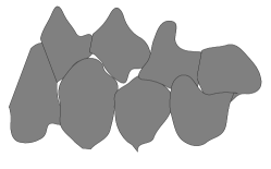
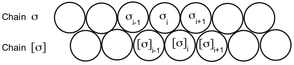
Figure 1: Schematic digram of F-actin strands. (a) Structure of actin detected by X-ray fiber diffraction. Adapted from Oda et al. [2009]. (b) Actin automata.

Each G-actin molecule (except those at the ends of F-actin strands) has four neighbours, as demonstrated in Fig. 1. An actin automaton consists of two chains $\sigma$ and $[\sigma]$ of semi-totalistic binary-state automata. Each automaton takes two states ‘0’ (resting) and ‘1’ (excited).

Conventional (Markovian) actin CA rules have been proposed to be implemented in two coupled layers (noted $\sigma$ and $[\sigma]$) with semitotalistic rules Adamatzky & Mayne [2014] :

$$\sigma^{(T+1)}_{i}=\left\{\begin{array}[]{lll}\vspace{0.25cm}\phi(\sigma^{(T)}_{i-1}+\sigma^{(T)}_{i+1}+[\sigma^{(T)}_{i}]+[\sigma^{(T)}_{i-1}])&if&\sigma^{(T)}_{i}=0\\ \psi(\sigma^{(T)}_{i-1}+\sigma^{(T)}_{i+1}+[\sigma^{(T)}_{i}]+[\sigma^{(T)}_{i-1}])&if&\sigma^{(T)}_{i}=1\end{array}\right.$$ (8c)

$$\vspace{0.5cm}[\sigma^{(T+1)}_{i}]=\left\{\begin{array}[]{lll}\vspace{0.25cm}\phi([\sigma^{(T)}_{i-1}]+[\sigma^{(T)}_{i+1}]+\sigma^{(T)}_{i}+\sigma^{(T)}_{i+1})&if&[\sigma^{(T)}_{i}]=0\\ \psi([\sigma^{(T)}_{i-1}]+[\sigma^{(T)}_{i+1}]+\sigma^{(T)}_{i}+\sigma^{(T)}_{i+1})&if&[\sigma^{(T)}_{i}]=1\end{array}\right.$$ (8f)

With the subrules $(\phi,\psi)$ expressed in binary and decimal forms as $\phi=(\beta_{0}\beta_{1}\beta_{2}\beta_{3}\beta_{4})\equiv\displaystyle{\sum^{4}_{i=0}2^{4-i}\beta_{i}}$ , and $\psi=(\gamma_{0}\gamma_{1}\gamma_{2}\gamma_{3}\gamma_{4})\equiv\displaystyle{\sum^{4}_{i=0}2^{4-i}\gamma_{i}}$ .

Actin CA rules with memory will be implemented from (8) as :

$$\sigma^{(T+1)}_{i}=\left\{\begin{array}[]{lll}\vspace{0.25cm}\phi(s^{(T)}_{i-1}+s^{(T)}_{i+1}+[s^{(T)}_{i}]+[s^{(T)}_{i-1}])&if&s^{(T)}_{i}=0\\ \psi(s^{(T)}_{i-1}+s^{(T)}_{i+1}+[s^{(T)}_{i}]+[s^{(T)}_{i-1}])&if&s^{(T)}_{i}=1\end{array}\right.$$ (9c)

$$\vspace{0.5cm}[\sigma^{(T+1)}_{i}]=\left\{\begin{array}[]{lll}\vspace{0.25cm}\phi([s^{(T)}_{i-1}]+[s^{(T)}_{i+1}]+s^{(T)}_{i}+s^{(T)}_{i+1})&if&[s^{(T)}_{i}]=0\\ \psi([s^{(T)}_{i-1}]+[s^{(T)}_{i+1}]+s^{(T)}_{i}+s^{(T)}_{i+1})&if&[s^{(T)}_{i}]=1\end{array}\right.$$ (9f)

Figure 2 shows the effect of memory up to $T=150$ in two actin rules when starting at random, i.e., the values of sites are initially uncorrelated and chosen at random to be 0 (blank) or 1 (black) with probability 1/2 in layers of size $n=300$ . The pictures show also the differences in patterns resulting from reversing the initial center site value. The perturbed region is enhanced with red pixels, corresponding to the site values that differed among the patterns generated with the two initial configurations. In the top frame of Fig. 2 , the actin rule R(10,10) is shown with ahistoric (left), $\tau=3$ and $\tau=100$-majority memory models. In the bottom frame, the rule R(14,9) is considered, with ahistoric (left), $\alpha=0.51$ and $\alpha=0.9$ memory models. The inertial (or conservative) effect that memory exerts tends to slow down propagation of growing patterns (perturbations, excitations). This is ‘slowing down’ is manifested by apparent ‘shrinking of patterns’ no the space-time configurations. This is so even with low memory charge, either in the form $\tau=3$ or as $\alpha=0.51$, but becomes fully appreciable with high memory (either $\tau=100$, or $\alpha=0.90$). In correspondence, the perturbation spreading in Fig. 2 becomes highly restrained as the memory charge increases, so that with high memory charge it remains confined to the proximity of its initial seed.

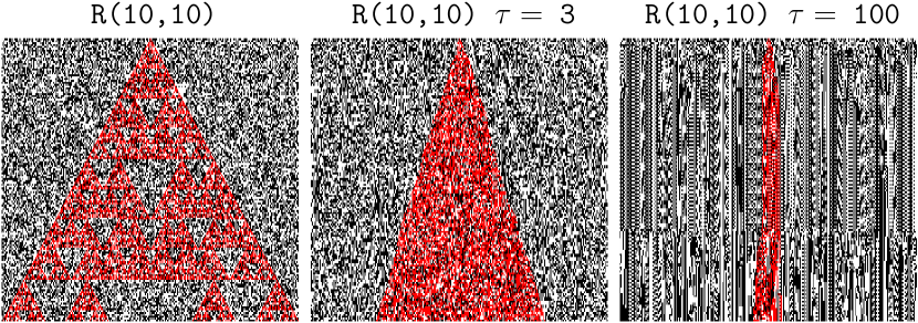
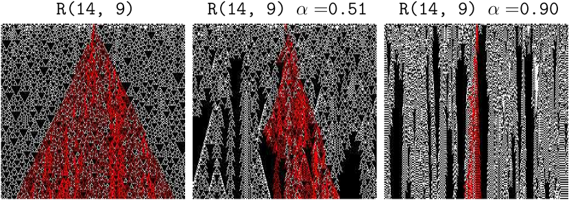
Figure 2: Dynamics in two actin rules up to $T=150$ . Top : Rule R(10,10). Ahistoric (left) and majority memory models. Bottom : Rule R(14,9). Ahistoric (left) and $\alpha$-memory models.

Figure 3 shows the effect of memory up to $T=1000$ in the actin rule (14,9) when starting at random in layers of size 1500 . In the $\alpha$ memory type (top snapshots), even the very low memory charge $\alpha=0.51$ dramatically alters the conventional (ahistoric) spatio-temporal patterns, with stationary localisations becoming dominating, whereas when $\alpha$ increases to 0.6 a sophisticated spatio-temporal pattern emerges where travelling glider guns produce gliders, and gliders reflect or annihilate in their collisions. With majority memory (bottom snapshots), the low memory charge $\tau=$ induces a monotonous transition between from enormous amount of gliders generated (so many that space is almost completely filled with them), to situation when few stationary glider guns generate gliders with low frequency, gliders collide and in most cases annihilate. When $\tau$ reaches 8 only stationary (breathing) localisations persist.

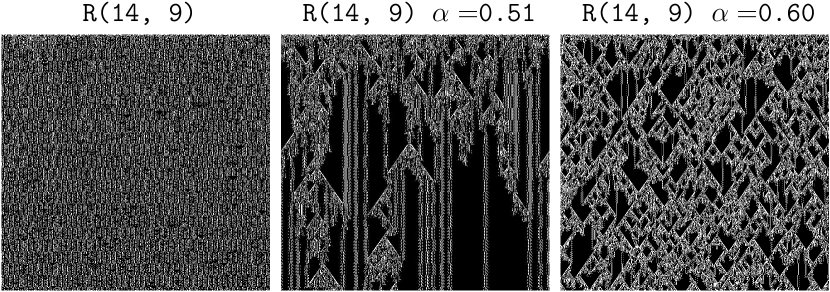
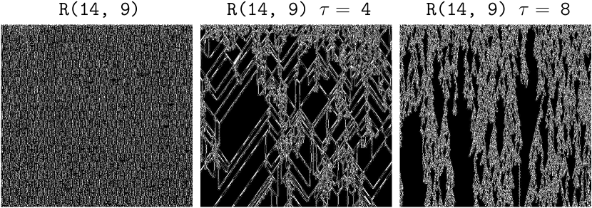
Figure 3: Dynamics in the rule R(14,9). Top : $\alpha$-memory, Bottom : majority memory.

The richness of the effect of memory may be envisaged in Fig .4 , where rule R(14,9) starts from one site active seed. Sophisticated patterns emerge bith the $\alpha$ and majority scenarios shown in Fig .4 .

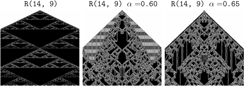
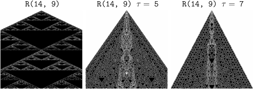
Figure 4: Dynamics in the rule R(14,9) starting from one site active seed. Top : $\alpha$-memory, Bottom : majority memory.

4 Global characteristics

Following the reference Adamatzky & Mayne [2014], the following integral measures are calculated on the spatio-temporal pattern $M=(m_{ti})$, where $m_{ti}$ is the state of the cell $i$ at time-step $t$ :

• Shannon entropy : $H=-\displaystyle\sum_{w\in W}\nu(w)/\eta\ln(\nu(w)/\eta)$

  Where $\eta$ is the sum of the $W$ possible kinds of $3\times 3$ configurations found in $M$ , and $\nu(w)$ is the number of times that the configuration $w$ is found in $M$ .

• Simpson diversity : $D=1-\displaystyle\sum_{w\in W}(\nu(w)/\eta)^{2}$

Figure 5 shows the entropy ($H$) versus diversity ($D$) in the left frames, and the distribution of the number of rules ($\#$) of given entropy. Ahistoric (black-marked) and $\tau$-majority memory (red-marked) models are in runs up to $T=1000$ are considered in Fig. 5 : Top : $\tau=3$, Middle : $\tau=100$, Bottom : $\tau=1000$ . Memory seems not to dramatically alter the form of the $H$-$D$ plots, at least at a first visual glance in the left panels of Fig. 5 , where the data from the ahistoric and memory simulations appear rather masked. At variance with this, memory appears to notably modify the distribution of the number of rules corresponding to the different levels of entropy in the right panels. Thus, comparing the ahistoric (or even the low level $\tau=3$ memory charge) to the full memory implementation in the bottom-right panel, it becomes apparent that the highest levels of entropy, close to 6.0, become with no rules filling them in the full memory implementation, whereas most of the rules correspond to the middle level H-interval [2.5,3.5] , an interval fairly low represented in the ahistoric scenario. Let us take the example of rule R(10,10). In the ahistoric model, R(10,10) achieves the entropy $H=6.233$, very close to the maximum attainable $H^{*}=\ln 2^{9}=6.238$ . With $\tau=3$ majority memory the entropy of R(10,10) is lowered to $H=6.005$, and with full memory to $H=5.335$ . In the scenarios of Fig. 5  the actin rule R(14,9) achieves in ahistoric model the entropy 3.342, which atypically increases, albeit very little, to 3.835 with $\tau=3$, then decreases to 3.199 with full memory.

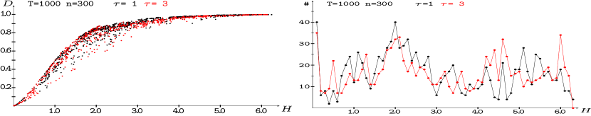
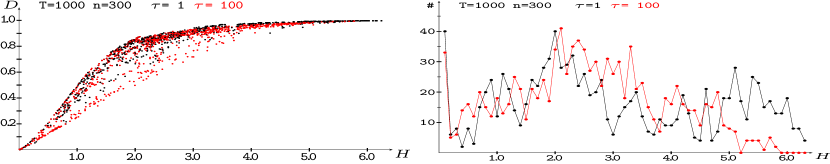
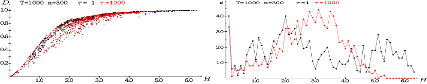
Figure 5: Entropy ($H$) versus diversity ($D$) (left) and entropy ($H$) versus number of rules ($\#$) (right) plots. Ahistoric (black) and $\tau$- majority (red) memory models. Top : $\tau=3$; Middle : $\tau=100$; Bottom : $\tau=1000$ .

5 Localizations

We provide additional section on localisations in acting automata with memory for the following reasons. Actin filaments are polyelectrolytes surrounded by counter-ions, the filaments therefore possess the capacity of transmitting signals or sustaining ionic conductances Cantiello et al. [1991]; Tuszyński et al. [2004]. Actin filaments, being rod-like polymers, are particularly likely to have counter-ions adsorbed to their surface at high ionic concentrations, such as those in the intra-neuronal environment, ions would be expected to densely adsorb to the surface of actin filaments due to complementary charges Priel et al. [2010]. The actin filaments are also capable for supporting propagation of discrete breathers (non-linear localised modes of excitation) as a consequence of nonlinearity in pure, translationally invariant systems of any dimensionality (similar to intrinsic localized modes in anharmonic crystals) Flach & Willis [1998]; Kavitha et al. [2013]; Kovaleva & Manevitch [2012]. The solitonic signals propagating on actin networks are capable of realising collision-based logical circuits Adamatzky [2001, 2000, 2004].

We consider three types of localisations:

• glider: travelling localisation, analogues to voltage solitons in cable equation model of actin Tuszyński et al. [2004], and discrete travelling breathers Flach & Willis [1998].

• still life: still stationary patterns, which repeats itself in every time, analogues to a standing wave, or localised excitation in vibrating granular material Umbanhowar et al. [1996]

• oscillator: oscillating stationary localisation, a pattern which repeats itself in a finite number of evolution steps; a glider also repeated itself but it is not stationary), stationary breather Flach & Willis [1998] or immobile voltage soliton Tuszyński et al. [2004].

Glider and still life are oscillators as well: a glider is translating oscillator and a still life is stationary oscillator period 1. We compare localisations generated by seeds of five scells in automata without memory and with memory. Given a rule $\mathcal{R}$ we say ‘glider becomes oscillator’ if an automaton governed by rule $\mathcal{R}$ evolves seed $s$ into a glider when it does not have memory and the automaton evolves the seed $s$ into a breather when the rule $\mathcal{R}$ is enriched with memory.

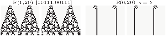
Figure 6: Spreading pattern is localised into a still life. Transformation of localisations by majority memory. In each subfigure we see space-time configurations of both actin chains in automata without memory (left) and with memory (right). Times goes down. Rules are indicated above the space-time configurations. Seeds are indicated in the label of the left (ahistoric) simulation.

As we discussed before, introduction of memory typically ‘shrinks’ patterns. In some rules, e.g. $R(6,20)$ the spreading pattern is shrunk to a still life occupying just one cell (Fig. 6).

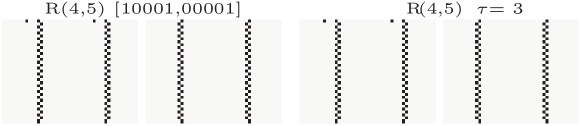
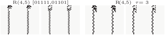
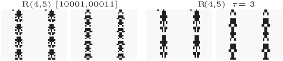
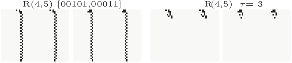
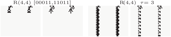
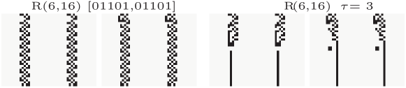
Figure 7: Transformation of oscillators by $\tau=3$ majority memory. In each subfigure we see space-time configurations of both actin chains in automata without memory (left) and with memory (right). Times goes down. Rules are indicated above the space-time configurations. (a) Oscillator is preserved. (b ) Oscillator remains yet frequency of its oscillation (breathing) decreases. (c ) Pattern of oscillations changes. (d) Oscillator is annihilated by memory. (e) Oscillator emerges assisted by memory. (f) Oscillator is transformed into still life. Seeds are indicated in the label of the left (ahistoric) simulation.

Oscillating stationary localisation is preserved (Fig. 7a), sometimes with decrease of oscillation frequency (Fig. 7b) or change of the oscillations pattern (Fig. 7c) or annihilated (Fig. 7d). In some rules oscillators can emerge, when state-transition rules are enriched with memory, e.g. in (Fig. 7d) a seed produces an extinguishing pattern in memoryless automaton yet it produces oscillator when majority memory is introduced. In rule $R(6,16)$ introduction of memory converts oscillator into a still life.

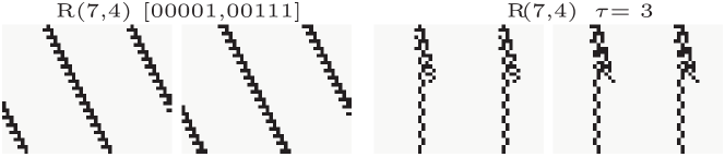
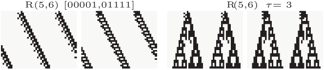
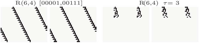
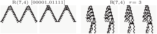
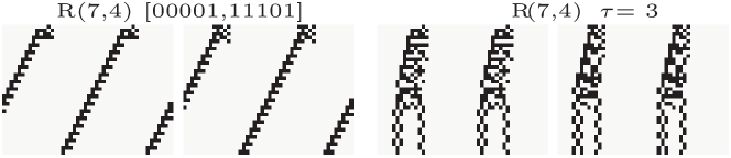
Figure 8: Transformation of gliders by $\tau=3$ majority memory. In each subfigure we see space-time configurations of both actin chains in automata without memory (left) and with memory (right). Times goes down. Rules are indicated above the space-time configurations. (a) Glider becomes oscillator. (b) Glider becomes a propagating and expanding pattern (Sierpinski gasket in this particular example). (c ) Glider is annihilated. (d) Glider propagating left is transformed into larger slow moving glider and glider propagating right becomes a oscillator. (e) Glider ‘splits’ into two breathers.

Gliders are transformed as follows (Fig. 8). Glider can be transformed to a oscillator (Fig. 8a), or expanding pattern (we can say that the glider was exploded by memory, Fig. 8b), or annihilated (Fig. 8c). In some cases, where a seed generates two gliders – one travels left and another travels right – one of the gliders becomes larger and slow moving glider while another glider is transformed into an oscillator (Fig. 8d); or, a single gliders is transformed into two oscillators with different patterns of oscillations (Fig. 8e).

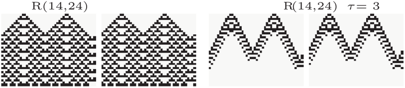
Figure 9: Initial configurations not of the 5-seed type. A spreading pattern is trimmed to gliders. Transformation of gliders by majority memory. In each subfigure we see space-time configurations of both actin chains in automata without memory (left) and with $\tau=3$-memory (right). Times goes down. Rules are indicated above the space-time configurations. Seeds :[00110000000000000000000110 , 01100000000000000000001100]

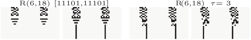
Figure 10: Entrainment. Dynamics of actin chains is asynchronous in rules without memory: still life persists only one chain. When memory is introduced both chains host still lifes. In each subfigure we see space-time configurations of both actin chains in automata without memory (left) and with $\tau=3$-memory (right). Times goes down. Rules are indicated above the space-time configurations.

In rare cases, e.g. rule $R(14,24)$ a spreading pattern is converted to two gliders, propagating to the left and to the right. The gliders annihilate when collide (Fig. 9). We can also observe an entrainment phenomenon (Fig. 10) where a localisation ‘inhabiting’ only one chain in a rule without memory, spreads to the second chain when memory is introduced.

Figure 11: Memory-induced transformations of localisation.

By undertaking exhaustive analysis of the rules we found that only the following transformations of localisations are possible when state transition rules are enriched with memory (Fig. 11). A glider is transformed to an oscillator. An oscillator is transformed to a still life. In some cases memory preserved gliders, oscillators and still life. Transformations of still lifes to oscillators or glider, and oscillations to gliders have not been observed so far. Notably, in elementary cellular automata with memory transitions from glider to oscillation to still life, induced by memory, could be found DBLP:journals/fuin/MartinezAA15; martinez2010make; martinez2012complex. We did not such transitions in actin automata with memory, this could be due to the fact interaction between two one-dimensional automata forming acting filament leads to ‘inhibition’ of glider dynamics and prevents formation of mobile localisations when memory is introduced to node state-transition rules.

6 Discussion

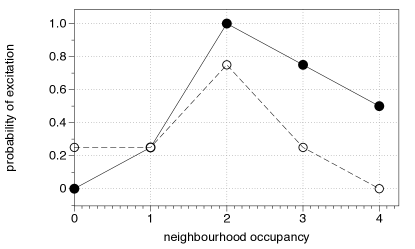
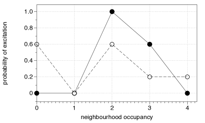
Figure 12: Dependence of a probability of excitation of a node in actin automaton (a) supporting travelling localizations and (b) supporting stationary localizations on a number of excited neighbours of the node. The plots are calculated for rules R(7,4), R(5,6), R(6,4), R(12,24), which support travelling localisations shown in Figs. 8, 9, 13, and rules R(6,20), R(4,5), R(4,4), R(6,16), R(6,18), which support stationary localisations shown in Fig. 6, 7, 10. Solid discs, connected by solid line, show probability of excitation of a resting node, circles, connected by dashed line, show probability of excitation of an excited node, i.e. of an excited node to remain excited.

In our original studies of actin automata (without memory) Adamatzky & Mayne [2015] we demonstrated, by exhaustive search of localisations over the whole rule space, that rule supports travelling localizations if a resting node excites if it has two or four excited neighbours and an excited node remains excited if it has no excited neighbours (there are indeed additional modes of excitability necessary to support propagation of the gliders). We also found that a rule supports stationary localizations if a resting node excites if it has three excited neighbours and an excited node remains excited if it has less than four excited neighbours. Analysing the rules of actin automat with majority, which we used to illustrate transformation of travelling and stationary localisations, we found that two excited neighbours is a necessary prerequisite for a resting node to be excited and for an excited node to remain excited for a rule to support travelling (Fig. 12a) and stationary (Fig. 12b) localisations. Second most common occupancy for these rules is three excited neighbours.

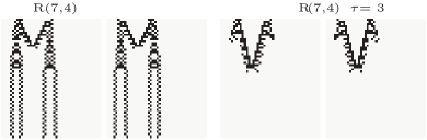
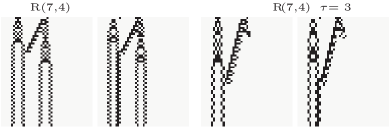
Figure 13: Initial configurations not of the 5-seed type. Interactions of localizations of rule R(7,4) with (right) and without (left) $\tau=3$ majority memory. (a) Two gliders collide and annihilate in the result of the collision. (b) Glider is stopped by oscillator. In each subfigure we see space-time configurations of both actin chains in automata. Seeds : (a) [0011100000000000001,0100000000000001110]  (b) [11100000000000001,00000010000000111]

By enriching actin automata with memory we demonstrated that when local transitions rules are enriched with memory they generate slower propagation or expanding patterns, generate less ‘complex’, as measured by entropies, space-time configurations. The memory enrichment also leads to transformation of gliders to oscillatory stationary localisations to still stationary localisations. These results well complement our previous findings in abstract analysis of intracellular acting filaments and complement parallel developments, such as extensions of actin automata to quantum actin automata Siccardi & Adamatzky [2015] and cable equations models of voltage solitons in actin Siccardi et al. [2015]. Gliders are propagating signals. Stationary localisation are memory — in a sense of volatile computer memory. So by varying depth of actin units memory we can force actin filaments either to produce signals — which compute when collide — or to act as a memory device. Basic computing properties of the quantum actin automata — Boolean logic gates and binary adder Siccardi & Adamatzky [2015], and three valued logic operations Adamatzky [2011] — have not yet been matched in the actin automata memory. These will topics of our further studies.

Right now we can just demonstrate interactions which can be interpreted in terms of collision-based computing: presence of a localisation indicate logical True and absence — logical False. A ‘classical’ annihilation gate $\langle x,y\rangle\rightarrow\langle\overline{x}y,x\overline{y}\rangle$ is shown in Fig. 13a for inputs $x=$True and $y=$False. When $x=$True there is a glider travelling right, when $y=$True there is a glider travelling left. If just one glider present in the gate, it continue it movement undisturbed. The trajectory of undisturbed movement of the glider travelling right represents $x\overline{y}$ and the trajectory of undisturbed movement of the glider travelling left represents $\overline{x}y$. Travelling localisations, representing data and result of computation can be stopped via stationary oscillators. An example is shown in Fig. 13b. Glider travels left. It collides into a oscillator. The oscillator changes its states in the result of collision. Thus travelling data are re-written into stationary data.

Figure 14: Emergence of localisation induced by memory, rule R(12,24). Distance between glider seeds is (a) 48 nodes and (b) 51 nodes. In each subfigure we see space-time configurations of both actin chains in automata without memory (left) and with $\alpha=0.55$-memory (right). Initially just single node is in state ‘1’. Times goes down. Rules are indicated above the space-time configurations.

Another example of memory-induced emergence of collision-based gates is illustrated in Fig. 14. In actin automata rule R(14,24) seeds of a single node in state ‘1’ develop into propagating patterns of regular ‘excitations’ of the actin filaments. When memory is introduced the interior of the propagating patterns is ‘filtered out’ and only wave-fronts, i.e. gliders, remain. The gliders reflect and change their phases when a distance between seeds is 48 nodes (Fig. 14a) and the gliders annihilate when the distance between seeds is 51 nodes (Fig. 14b).

References

- Adamatzky [2000] Adamatzky, A. [2000] “Collision-based computing in biopolymers and their automata models.” International Journal of Modern Physics C 11, 1321–1346.
- Adamatzky [2001] Adamatzky, A. [2001] Computing in nonlinear media and automata collectives (CRC Press).
- Adamatzky [2004] Adamatzky, A. [2004] “Collision-based computing in belousov–zhabotinsky medium,” Chaos, Solitons & Fractals 21, 1259–1264.
- Adamatzky [2011] Adamatzky, A. [2011] “Topics in reaction-diffusion computers.” Journal of Computational and Theoretical Nanoscience 8, 295–303.
- Adamatzky & Mayne [2014] Adamatzky, A. & Mayne, R. [2014] “Actin automata: Phenomenology and localizations,” arxiv .
- Adamatzky & Mayne [2015] Adamatzky, A. & Mayne, R. [2015] “Actin automata: Phenomenology and localizations,” International Journal of Bifurcation and Chaos 25, 1550030, 10.1142/S0218127415500303, URL http://www.worldscientific.com/doi/abs/10.1142/S0218127415500303.
- Alonso-Sanz [2011] Alonso-Sanz, R. [2011] Discrete systems with memory, Vol. 75 (World Scientific).
- Alonso-Sanz & Bull [2003] Alonso-Sanz, R. & Bull, L. [2003] “One-dimensional coupled cellular automata with memory: Initial investigations.” J. Cellular automata 5, 29–49.
- Alonso-Sanz & Martin [2006] Alonso-Sanz, R. & Martin, M. [2006] “Elementary cellular automata with elementary memory rules in cells: The case of linear rules.” J. Cellular Automata 1, 71–87.
- Cantiello et al. [1991] Cantiello, H., Patenaude, C. & Zaner, K. [1991] “Osmotically induced electrical signals from actin filaments.” Biophysical journal 59, 1284.
- Cingolani & Goda [2008] Cingolani, L. A. & Goda, Y. [2008] “Actin in action: the interplay between the actin cytoskeleton and synaptic efficacy,” Nature Reviews Neuroscience 9, 344–356.
- Conrad [1996] Conrad, M. [1996] “Cross-scale information processing in evolution, development and intelligence,” BioSystems 38, 97–109.
- Debanne [2004] Debanne, D. [2004] “Information processing in the axon,” Nature Reviews Neuroscience 5, 304–316.
- Dillon & Goda [2005] Dillon, C. & Goda, Y. [2005] “The actin cytoskeleton: integrating form and function at the synapse,” Annu. Rev. Neurosci. 28, 25–55.
- Fiala et al. [2002] Fiala, J. C., Spacek, J. & Harris, K. M. [2002] “Dendritic spine pathology: cause or consequence of neurological disorders?” Brain Research Reviews 39, 29–54.
- Fifková & Delay [1982] Fifková, E. & Delay, R. J. [1982] “Cytoplasmic actin in neuronal processes as a possible mediator of synaptic plasticity.” The Journal of Cell Biology 95, 345–350.
- Flach & Willis [1998] Flach, S. & Willis, C. R. [1998] “Discrete breathers,” Physics reports 295, 181–264.
- Hameroff [1988] Hameroff, S. [1988] “Coherence in the cytoskeleton: Implications for biological information processing,” Biological coherence and response to external stimuli (Springer), pp. 242–265.
- Hameroff [1998] Hameroff, S. [1998] “Quantum computation in brain microtubules? the penrose-hameroff ‘orch or’ model of consciousness.” Philosophical Transactions of the Royal Society of London A 356, 1869–1896.
- Hameroff et al. [1992] Hameroff, S. R., Dayhoff, J. E., Lahoz-Beltra, R., Samsonovich, A. V. & Rasmussen, S. [1992] “Models for molecular computation: conformational automata in the cytoskeleton,” Computer 25, 30–39.
- Jaeken [2007] Jaeken, L. [2007] “A new list of functions of the cytoskeleton,” IUBMB life 59, 127–133.
- Janmey [1998] Janmey, P. [1998] “The cytoskeleton and cell signalling: component localization and mechanical coupling.” Physiological Reviews 78, 763–781.
- Kavitha et al. [2013] Kavitha, L., Muniyappan, A., Prabhu, A., Zdravković, S., Jayanthi, S. & Gopi, D. [2013] “Nano breathers and molecular dynamics simulations in hydrogen-bonded chains,” Journal of biological physics 39, 15–35.
- Kim & Lisman [1999] Kim, C.-H. & Lisman, J. E. [1999] “A role of actin filament in synaptic transmission and long-term potentiation,” The Journal of neuroscience 19, 4314–4324.
- Kojima & Shirao [2007] Kojima, N. & Shirao, T. [2007] “Synaptic dysfunction and disruption of postsynaptic drebrin–actin complex: a study of neurological disorders accompanied by cognitive deficits,” Neuroscience research 58, 1–5.
- Kovaleva & Manevitch [2012] Kovaleva, N. & Manevitch, L. [2012] “Analytical study of discrete optical breathers in spiral polymer chain,” Macromolecular Theory and Simulations 21, 516–528.
- Ludin & Matus [1993] Ludin, B. & Matus, A. [1993] “The neuronal cytoskeleton and its role in axonal and dendritic plasticity,” Hippocampus 3, 61–71.
- Oda et al. [2009] Oda, T., Iwasa, M., Aihara, T., Maéda, Y. & Narita, A. [2009] “The nature of the globular-to fibrous-actin transition,” Nature 457, 441–445.
- Persico & Bourgeron [2006] Persico, A. M. & Bourgeron, T. [2006] “Searching for ways out of the autism maze: genetic, epigenetic and environmental clues,” Trends in neurosciences 29, 349–358.
- Priel et al. [2006] Priel, A., Tuszynski, J. A. & Cantiello, H. F. [2006] “The dendritic cytoskeleton as a computational device: an hypothesis,” The Emerging Physics of Consciousness (Springer), pp. 293–325.
- Priel et al. [2010] Priel, A., Tuszynski, J. A. & Woolf, N. J. [2010] “Neural cytoskeleton capabilities for learning and memory,” Journal of biological physics 36, 3–21.
- Rasmussen et al. [1990] Rasmussen, S., Karampurwala, H., Vaidyanath, R., Jensen, K. S. & Hameroff, S. [1990] “Computational connectionism within neurons: A model of cytoskeletal automata subserving neural networks,” Physica D: Nonlinear Phenomena 42, 428–449.
- Sekino et al. [2007] Sekino, Y., Kojima, N. & Shirao, T. [2007] “Role of actin cytoskeleton in dendritic spine morphogenesis,” Neurochemistry international 51, 92–104.
- Siccardi & Adamatzky [2015] Siccardi, S. & Adamatzky, A. [2015] “Actin quantum automata: Communication and computation in molecular networks,” Nano Communication Networks 6, 15–27.
- Siccardi et al. [2015] Siccardi, S., Tuszynski, J. A. & Adamatzky, A. [2015] “Boolean gates on actin filaments,” arXiv preprint arXiv:1506.09044 .
- Tuszynski et al. [1998] Tuszynski, J., Brown, J. & Hawrylak, P. [1998] “Dielectric polarization, electrical conduction, information processing and quantum computation in microtubules. are they plausible?” Philosophical Transaction Royal Society of London. Series A: Mathematical, Physical and Engineering Sciences , 1897–1925.
- Tuszyński et al. [2004] Tuszyński, J., Portet, S., Dixon, J., Luxford, C. & Cantiello, H. [2004] “Ionic wave propagation along actin filaments,” Biophysical journal 86, 1890–1903.
- Umbanhowar et al. [1996] Umbanhowar, P. B., Melo, F. & Swinney, H. L. [1996] “Localized excitations in a vertically vibrated granular layer,” Nature 382, 793–796.
- van Spronsen & Hoogenraad [2010] van Spronsen, M. & Hoogenraad, C. C. [2010] “Synapse pathology in psychiatric and neurologic disease,” Current neurology and neuroscience reports 10, 207–214.
- Van Woerkom [1990] Van Woerkom, A. [1990] “The major hallucinogens and the central cytoskeleton: an association beyond coincidence? towards sub-cellular mechanisms in schizophrenia,” Medical hypotheses 31, 7–15.