Higgs boson production in the $U(1)_{B-L}$ model at the ILC

Abstract

In the framework of the minimal $U(1)_{B-L}$ extension of the Standard Model, we investigate the Higgs boson production processes $e^{+}e^{-}\rightarrow ZH$, $e^{+}e^{-}\rightarrow\nu_{e}\bar{\nu_{e}}H$, $e^{+}e^{-}\rightarrow t\bar{t}H$, $e^{+}e^{-}\rightarrow ZHH$ and $e^{+}e^{-}\rightarrow\nu_{e}\bar{\nu_{e}}HH$ at the International Linear Collider (ILC). We present the production cross sections, the relative corrections and compare our results with the expected experimental accuracies for Higgs decay channel $H\rightarrow b\bar{b}$. In the allowed parameter space, we find that the effects of the three single Higgs boson production processes might approach the observable threshold of the ILC. But the Higgs signal strengths $\mu_{b\bar{b}}$ of the two double Higgs boson production processes are all out of the observable threshold so that these effects will be difficult to be observed at the ILC.

I Introduction

In the summer of 2012, a bosonic resonance with a mass around 125 GeV was found at the Large Hadron Collider (LHC) by the ATLAS and CMS Collaborations ATLAS-H ; CMS-H . So far, its properties are compatible with the predictions of the Standard Model (SM) Higgs boson. Meanwhile, the current LHC data is limited, there are still large uncertainties about the couplings between the Higgs boson and the other SM particles LHC-1 ; LHC-2 ; LHC-3 ; LHC-4 ; LHC-5 . Due to the complicated background, the precision measurements of the properties of the Higgs boson at the LHC are severely challenged. By contrast, the Higgs factories beside the LHC, such as the International Linear Collider (ILC) ILC-1 ; ILC-2 ; ILC-3 , can measure the Higgs boson with high accuracy. In many cases, the ILC can significantly improve the LHC measurements due to its clean environment.

The ILC technical design report has pointed that it is planed to measure Higgs boson at three center-of-mass (c.m.) energy: 250 GeV, 500 GeV and 1000 GeV. In the first stage for $\sqrt{s}=250$ GeV, the precision Higgs program will start at the Higgs-strahlung process $e^{+}e^{-}\rightarrow ZH$, the cross section for this process is dominant at the low energy and has the maximum cross section at around $\sqrt{s}=250$ GeV. In the second stage for $\sqrt{s}=500$ GeV, the two very important processes $e^{+}e^{-}\rightarrow t\bar{t}H$ and $e^{+}e^{-}\rightarrow ZHH$ are become accessible. For the process $e^{+}e^{-}\rightarrow t\bar{t}H$, in which the top Yukawa coupling appears at the tree-level for the first time at the ILC, it will play an important role for the precision measurements of the top quark Yukawa coupling. For the process $e^{+}e^{-}\rightarrow ZHH$, to which the triple Higgs boson coupling contributes at the tree-level, it will be crucial to understand the Higgs self-coupling and the electroweak symmetry breaking. In the third stage for $\sqrt{s}=1000$ GeV, the processes $e^{+}e^{-}\rightarrow t\bar{t}H$, $e^{+}e^{-}\rightarrow\nu_{e}\bar{\nu_{e}}H$ and $e^{+}e^{-}\rightarrow\nu_{e}\bar{\nu_{e}}HH$ are involved. In such energy stages, the channels $t\bar{t}H$ and $\nu_{e}\bar{\nu_{e}}H$ have large cross section, and the channel $\nu_{e}\bar{\nu_{e}}HH$ can be used together with the $ZHH$ process to improve the measurement of the Higgs self-coupling. So far, many relevant works mentioned above have been extensively studied in the context of the SM SM-zh-vvh-eeh-1 ; SM-zh-vvh-eeh-2 ; SM-zh-vvh-eeh-3 ; SM-zh-vvh-eeh-4 ; SM-zh-vvh-eeh-5 ; SM-zh-vvh-eeh-6 ; SM-zh-vvh-eeh-7 and some new physics models np-1 ; np-2 ; np-3 ; np-4 ; np-5 ; np-6 ; np-7 ; np-8 ; np-9 ; np-10 ; np-11 ; np-12 ; np-13 ; np-14 ; np-15 ; np-16 ; np-17 ; np-18 ; np-19 ; np-20 .

The minimal $B-L$ extension of the SM is based on the structure $SU(3)_{C}\times SU(2)_{L}\times U(1)_{Y}\times U(1)_{B-L}$ gauge symmetry, in which the SM gauge has a further $U(1)_{B-L}$ group related to the Baryon minus Lepton $(B-L)$ gauged number B-L-1 ; B-L-2 . It was known that this model is in agreement with the current experimental results of the light neutrino masses and their large mixing. The $B-L$ model predicted some new particles beyond the SM, such as the new heavy gauge bosons, the heavy neutrino and the heavy neutral Higgs boson. In addition, some couplings of the Higgs boson in the $B-L$ model are modified with respect to the SM. These new effects will alter the property of the SM Higgs boson and influence various SM Higgs boson processes, making the model phenomenologically rich and testable at the LHC and the ILC B-L-2 ; B-L-LHC-ILC-1 ; B-L-LHC-ILC-2 ; B-L-LHC-ILC-3 ; B-L-LHC-ILC-4 ; B-L-LHC-ILC-5 ; B-L-LHC-ILC-6 ; B-L-LHC-ILC-7 ; B-L-LHC-ILC-8 ; B-L-LHC-ILC-9 ; B-L-LHC-ILC-10 . In this paper, we mainly study the single Higgs boson production processes $e^{+}e^{-}\rightarrow ZH$, $e^{+}e^{-}\rightarrow\nu_{e}\bar{\nu_{e}}H$, $e^{+}e^{-}\rightarrow e^{+}e^{-}H$, $e^{+}e^{-}\rightarrow t\bar{t}H$ and the double Higgs boson production processes $e^{+}e^{-}\rightarrow ZHH$, $e^{+}e^{-}\rightarrow\nu_{e}\bar{\nu_{e}}HH$ in the $B-L$ model at the ILC.

The paper is organized as follows. In Sec.II we briefly review the basic content of the $B-L$ model related to our work. In Sec.III and Sec.IV we respectively investigate the Higgs boson production processes and the Higgs signal strengths in the $B-L$ model at the ILC. Finally, we give a summary in Sec.V.

II A brief review of the B-L model

Here we will briefly review the ingredients relevant to our calculations, the detailed description of the $B-L$ model can be found in Refs. B-L-LHC-ILC-1 ; B-L-LHC-ILC-4 . The $B-L$ model is the minimal extensions of the SM B-L-extension-1 ; B-L-extension-2 ; B-L-extension-3 ; B-L-extension-4 ; B-L-extension-5 with the classical conformal symmetry, and based on the gauge group $SU(3)_{C}\times SU(2)_{L}\times U(1)_{Y}\times U(1)_{B-L}$. The Lagrangian for the fermionic and kinetic sectors are given by

$$\mathcal{L}_{B-L} = i~{}\bar{l}D_{\mu}\gamma^{\mu}l+i~{}\bar{e}_{R}D_{\mu}\gamma^{\mu}e_{R}+i~{}\bar{\nu}_{R}D_{\mu}\gamma^{\mu}\nu_{R}$$ (1)

$$-\frac{1}{4}W_{\mu\nu}W^{\mu\nu}-\frac{1}{4}B_{\mu\nu}B^{\mu\nu}-\frac{1}{4}C_{\mu\nu}C^{\mu\nu}.$$

The covariant derivative $D_{\mu}$ is different from the SM one by the term $ig^{\prime}Y_{B-L}C_{\mu}$, where $g^{\prime}$ is the $U(1)_{B-L}$ gauge coupling constant, $Y_{B-L}$ is the $B-L$ charge, and $C_{\mu\nu}=\partial_{\mu}C_{\nu}-\partial_{\nu}C_{\mu}$ is the field strength of the $U(1)_{B-L}$.

The Lagrangian for the Higgs and Yukawa sectors are given by

$$\mathcal{L}_{B-L} = (D^{\mu}\phi)(D_{\mu}\phi)+(D^{\mu}\chi)(D_{\mu}\chi)-V(\phi,\chi)$$ (2)

$$-\Big{(}\lambda_{e}\bar{l}\phi e_{R}+\lambda_{\nu}\bar{l}\tilde{\phi}{\nu}_{R}+\frac{1}{2}\lambda_{\nu_{R}}\bar{\nu^{c}}_{R}\chi\nu_{R}+h.c.\Big{)}.$$

The $U(1)_{B-L}$ and $SU(2)_{L}\times U(1)_{Y}$ gauge symmetries can be spontaneously broken by a SM singlet complex scalar field $\chi$ and a complex $SU(2)$ doublet of scalar fields $\phi$, respectively.

The scalar potential $V(\phi,\chi)$ is given by

$$V(\phi,\chi) = m_{1}^{2}\phi^{\dagger}\phi+m_{2}^{2}\chi^{\dagger}\chi+\lambda_{1}(\phi^{\dagger}\phi)^{2}+\lambda_{2}(\chi^{\dagger}\chi)^{2}+\lambda_{3}(\chi^{\dagger}\chi)(\phi^{\dagger}\phi).$$ (3)

To determine the condition for the potential to be bounded from below, the couplings $\lambda_{1},\lambda_{2}$ and $\lambda_{3}$ should be related with $4\lambda_{1}\lambda_{2}-\lambda_{3}>0,\lambda_{1}\geq 0,\lambda_{2}\geq 0$. The vev’s, $|\langle\phi\rangle|=v/\sqrt{2}$ and $|\langle\chi\rangle|=v^{\prime}/\sqrt{2}$, are then given by

$$v^{2}=\frac{4\lambda_{2}m_{1}^{2}-2\lambda_{3}m_{2}^{2}}{\lambda_{3}^{2}-4\lambda_{1}\lambda_{2}},~{}\ \ \ \ ~{}~{}v^{\prime 2}=\frac{-2(m_{1}^{2}+\lambda_{1}v^{2})}{\lambda_{3}}.$$ (4)

where $v$ and $v^{\prime}$ are the electroweak symmetry breaking scale and the $B-L$ symmetry breaking scale, respectively.

After the electroweak symmetry breaking, one obtains the mass of the gauge bosons

$$m_{\gamma} =0,$$

$$m_{W^{\pm}} =\frac{1}{2}vg,$$

$$m_{Z} =\frac{v}{2}\sqrt{g^{2}+g_{1}^{2}},$$

$$m_{Z^{\prime}} =2v^{\prime}g^{\prime}.$$ (5)

where $g$ and $g_{1}$ are the $SU(2)_{L}$ and $U(1)_{Y}$ gauge couplings. The $Z^{\prime}$ boson mass is constrained from the most recent limit at LEP LEP-constrain

$$m_{Z^{\prime}}/g^{\prime}>7~{}{\rm TeV}.$$ (6)

The mixing between the SM complex $SU(2)_{L}$ doublet and complex scalar singlet is controlled by the coupling $\lambda_{3}$ as shown in Eq. (3). This mixing can be expressed by the mass matrix $\phi$ and $\chi$

$$\frac{1}{2}m^{2}(\phi,\chi)=\left(\begin{array}[]{cc}\lambda_{1}v^{2}&\frac{\lambda_{3}}{2}vv^{\prime}\\ \frac{\lambda_{3}}{2}vv^{\prime}&\lambda_{2}v^{\prime 2}\end{array}\right).$$ (7)

Therefore, the mass eigenstates fields $H$ and $H^{\prime}$ are given by

$$\left(\begin{array}[]{c}H\\ H^{\prime}\end{array}\right)=\left(\begin{array}[]{cc}\cos\alpha&-\sin\alpha\\ \sin\alpha&\cos\alpha\end{array}\right)\left(\begin{array}[]{c}\phi\\ \chi\end{array}\right),$$ (8)

where the mixing angle $\alpha$ is defined by

$$\tan 2\alpha=\frac{|\lambda_{3}|vv^{\prime}}{\lambda_{1}v^{2}-\lambda_{2}v^{\prime 2}}.$$ (9)

The masses of $H$ and $H^{\prime}$ are given by

$$m_{H,H^{\prime}}^{2}=\lambda_{1}v^{2}+\lambda_{2}v^{\prime 2}\mp\sqrt{(\lambda_{1}v^{2}-\lambda_{2}v^{\prime 2})^{2}+\lambda_{3}^{2}v^{2}v^{\prime 2}}.$$ (10)

Here, $H$ and $H^{\prime}$ are light and heavy Higgs bosons, respectively.

From Eqs. (9) and (10), it is straightforward to have:

$$\lambda_{1} = \frac{m_{H}^{2}}{2v^{2}}\cos^{2}{\alpha}+\frac{m_{H^{\prime}}^{2}}{2v^{2}}\sin^{2}{\alpha},$$

$$\lambda_{2} = \frac{m_{H}^{2}}{2{v^{\prime}}^{2}}\sin^{2}{\alpha}+\frac{m_{H^{\prime}}^{2}}{2{v^{\prime}}^{2}}\cos^{2}{\alpha},$$

$$\lambda_{3} = \frac{\left(m_{H^{\prime}}^{2}-m_{H}^{2}\right)}{2vv^{\prime}}\sin{(2\alpha)}.$$ (11)

Because of the mixing between the two Higgs bosons $H$ and $H^{\prime}$, the usual couplings among the SM-like Higgs $H$ boson and the SM particles are modified. Additionally, there are new couplings among the extra Higgs $H^{\prime}$ and the SM particles, which will lead to a different Higgs phenomenology from the SM. Notice that the scalar mixing angle $\alpha$ is a free parameter of the model, and the light(heavy) Higgs boson couples to the new matter content proportionally to sin$\alpha$ (cos$\alpha$). The relevant Feynman rules involved in our calculations are given in Table A.1 of App. A, which can be found in Refs. B-L-2 ; B-L-LHC-ILC-7 .

III Higgs productions in the B-L model at ILC

In our numerical calculations, we take the SM parameters as: $m_{t}=$172.4 GeV, ${\sin}^{2}\theta_{W}=$0.23126, $m_{Z}=$91.187 GeV, $m_{H}=$125 GeV, $\alpha(m_{Z})$=1/128 PDG-2014 . For the $B-L$ parameters, the mixing angle $\alpha$, the gauge coupling constant $g^{\prime}$, the mixing gauge coupling $\tilde{g}$, the masses $m_{Z^{\prime}}$, $m_{H^{\prime}}$ and $m_{\nu_{H}}$ are involved. The Ref.B-L-consition-1 has discussed the constraints on these parameters from experiment and theory, and points out that ${\rm sin}\alpha\leq 0.36$, $m_{Z^{\prime}}\geq 1830$ GeV, $m_{\nu_{H}}\sim 500~{}{\rm GeV}$, $m_{H^{\prime}}\geq 125~{}{\rm GeV}$. In the following calculations, we vary ${\rm sin}\alpha$ in the range of $0.05\leq{\rm sin}\alpha\leq 0.4$, and take $m_{Z^{\prime}}=2500~{}{\rm GeV}$, $m_{\nu_{H}}=500~{}{\rm GeV}$, $m_{H^{\prime}}=500~{}{\rm GeV}$, $g^{\prime}=0.3$, $\tilde{g}=-0.1$. All the numerical results are done by using CalcHEP 3.6.25 package calchep .

III.1 Single Higgs boson productions

In Fig.1 and Fig.2, we show the lowest-order Feynman diagrams of the single Higgs boson production processes $e^{+}e^{-}\rightarrow ZH$, $e^{+}e^{-}\rightarrow\nu_{e}\bar{\nu_{e}}H$ and $e^{+}e^{-}\rightarrow t\bar{t}H$ in the $B-L$ model. In comparison with the SM, we can see that these three processes receive the additional contributions from the heavy gauge boson $Z^{\prime}$ and the modified couplings of $HXX$ at the tree-level.

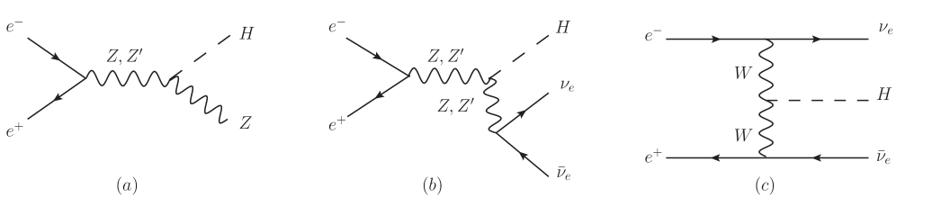
Figure 1: Lowest-order Feynman diagrams for $e^{+}e^{-}\rightarrow ZH$(a) and $e^{+}e^{-}\rightarrow\nu_{e}\bar{\nu_{e}}H$(b,c) in the $B-L$ model.

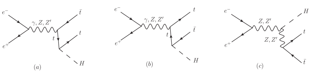
Figure 2: Lowest-order Feynman diagrams for $e^{+}e^{-}\rightarrow t\bar{t}H$ in the $B-L$ model.

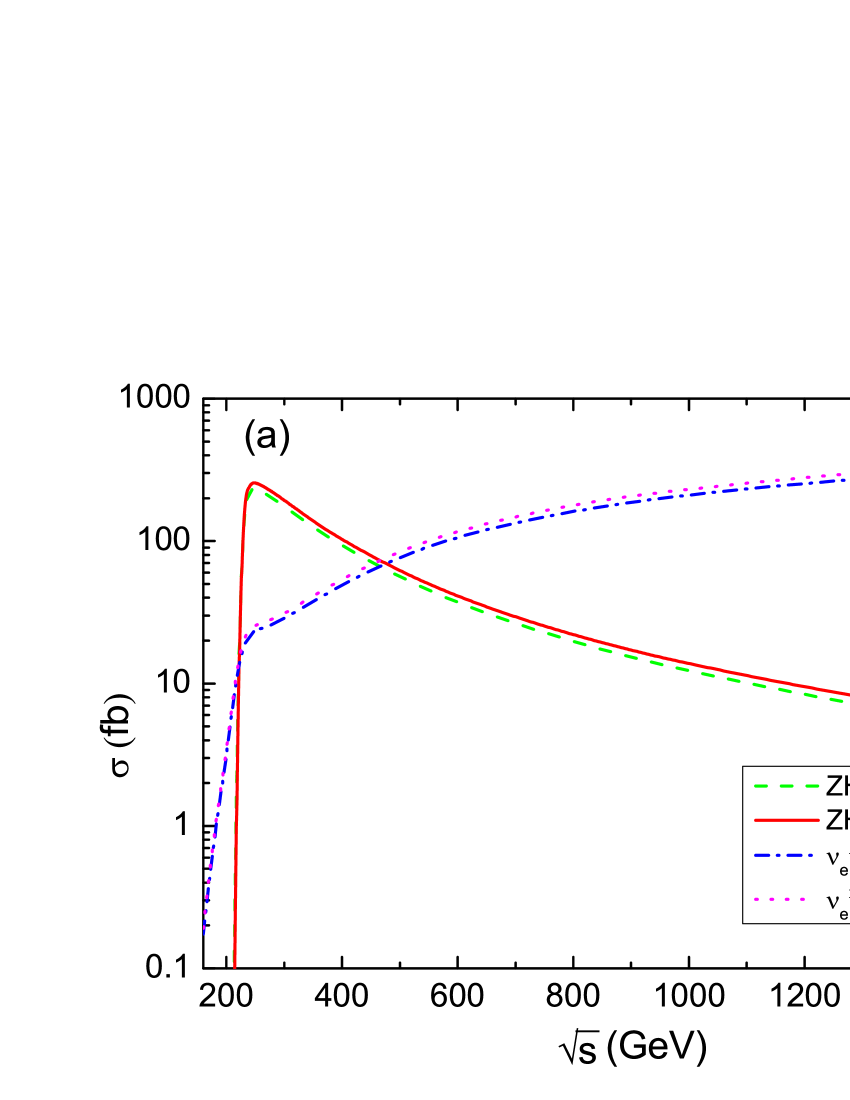
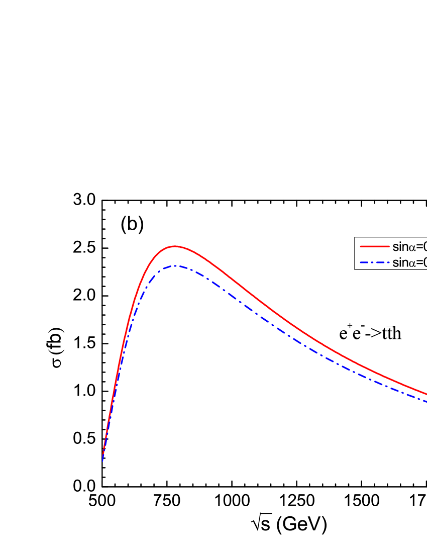
Figure 3: The production cross section $\sigma$ for the process $e^{+}e^{-}\rightarrow ZH$, $e^{+}e^{-}\rightarrow\nu_{e}\bar{\nu_{e}}H$ (a) and $e^{+}e^{-}\rightarrow t\bar{t}H$ (b) versus the c.m. energy $\sqrt{s}$ in the SM and $B-L$ model.

In Fig.3, we show the production cross sections $\sigma$ of these three processes versus the c.m. energy $\sqrt{s}$ in the SM and $B-L$ model, respectively. We can see that the process $e^{+}e^{-}\rightarrow ZH$ reaches its maximum at $\sim$ 250 GeV. The $\nu_{e}\bar{\nu_{e}}H$ production cross sections increase with the $\sqrt{s}$ and can take over that of the $ZH$ process at $\sqrt{s}\geq 500$ GeV. Similar to the process $e^{+}e^{-}\rightarrow ZH$, the $t\bar{t}H$ production cross sections increase firstly and then decrease with the $\sqrt{s}$ and reaches its maximum at $\sim$ 800 GeV. The cross sections of these three production processes in the $B-L$ model are all lower than their SM values.

Considering the polarization of the initial electron and positron beams, the cross section of a process can be expressed as polarization-1 ; polarization-2

$$\sigma(P_{e^{-}},P_{e^{+}}) = \frac{1}{4}[(1+P_{e^{-}})(1+P_{e^{+}})\sigma_{RR}+(1-P_{e^{-}})(1-P_{e^{+}})\sigma_{LL}$$ (12)

$$+(1+P_{e^{-}})(1-P_{e^{+}})\sigma_{RL}+(1-P_{e^{-}})(1+P_{e^{+}})\sigma_{LR}],$$

where $P_{e^{-}}$ and $P_{e^{+}}$ are the polarization degree of the electron and positron beam, respectively. As in Ref. ILC-2 , we assume $P(e^{-},e^{+})=(-0.8,0.3)$ at $\sqrt{s}$=250, 500 GeV and $P(e^{-},e^{+})=(-0.8,0.2)$ at $\sqrt{s}$=1000 GeV in our calculations.

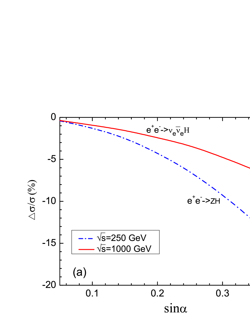
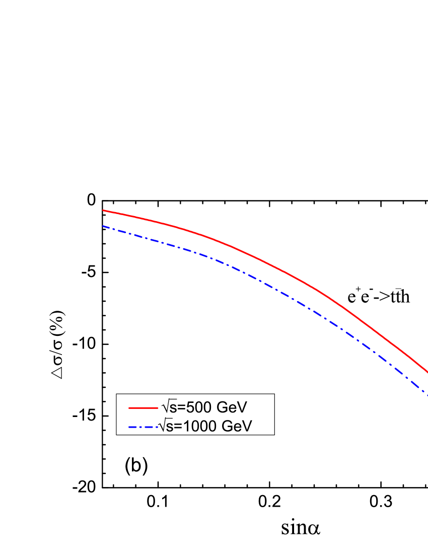
Figure 4: The relative correction $\Delta\sigma/\sigma$ for the process $e^{+}e^{-}\rightarrow ZH$, $e^{+}e^{-}\rightarrow\nu_{e}\bar{\nu_{e}}H$ (a) and $e^{+}e^{-}\rightarrow t\bar{t}H$ (b) versus ${\rm sin}\alpha$ for different c.m. energy $\sqrt{s}$ in the $B-L$ model.

In Fig.4, we show the relative corrections $\Delta\sigma/\sigma$=$(\sigma_{B-L}-\sigma_{SM})/\sigma_{SM}$ of the three single Higgs boson production channels versus the mixing angle ${\rm sin}\alpha$ for $\sqrt{s}=250,500,1000$ GeV at the ILC with polarized beams. For these three processes, we can see that the values of the relative corrections are all negative and increase with the ${\rm sin}\alpha$ increasing, the $\Delta\sigma/\sigma$ of processes $ZH$, $\nu_{e}\bar{\nu_{e}}H$, $t\bar{t}H$ can respectively reach $-16.2\%,-8.2\%,-16.4\%$. Due to the fact that the effects of the heavy gauge boson $Z^{\prime}$ decouple, the relative corrections $\Delta\sigma/\sigma$ are insensitive to the $m_{Z^{\prime}}$, so we do not show the dependence of the relative corrections on $m_{Z^{\prime}}$ here.

At the ILC with $\sqrt{s}$ = 250 GeV, the total SM electroweak correction for the $ZH$ production process is about 5% sm1 ; sm2 . Meanwhile, the ILC can measure the cross section for $ZH$ and $\nu_{e}\bar{\nu_{e}}H$ to a relative accuracy of $2.0-2.6\%$ and $2.2-11\%$ ILC-2 . At the ILC with $\sqrt{s}$ = 1000 GeV, the expected accuracies for $t\bar{t}H$ process may achieve an even more remarkable precision of 6.3%ILC-2 . Thus, the $B-L$ model effects on these three processes might be observed at the ILC for the large sin$\alpha$.

III.2 Double Higgs boson productions

At the ILC, the main triple Higgs boson coupling can be studied through the double Higgs-strahlung off $Z$ boson process $e^{+}e^{-}\rightarrow ZHH$ and double Higgs fusion process $e^{+}e^{-}\rightarrow\nu_{e}\bar{\nu_{e}}HH$. The relevant Feynman diagrams are shown in Fig.5 and Fig.6.

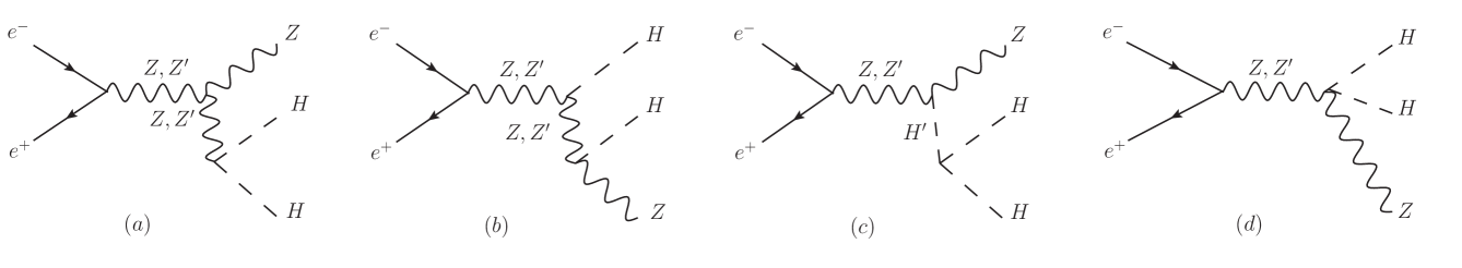
Figure 5: Lowest-order Feynman diagrams for $e^{+}e^{-}\rightarrow ZHH$ in the $B-L$ model.

In Fig.7(a), we show the cross sections for the two processes versus the c.m. energy $\sqrt{s}$ in the SM and the $B-L$ model for sin$\alpha$ = 0.3. We can see that the cross section for the process $e^{+}e^{-}\rightarrow ZHH$ reaches its maximum at around 500 GeV. It is noteworthy that the process $e^{+}e^{-}\rightarrow\nu_{e}\bar{\nu_{e}}HH$ will become sizable at $\sqrt{s}$ = 1000 GeV and can be used together with the $e^{+}e^{-}\rightarrow ZHH$ process to improve the measurement of the Higgs self-coupling. Furthermore, we can see that the two processes have a similar trend in the SM and the $B-L$ model.

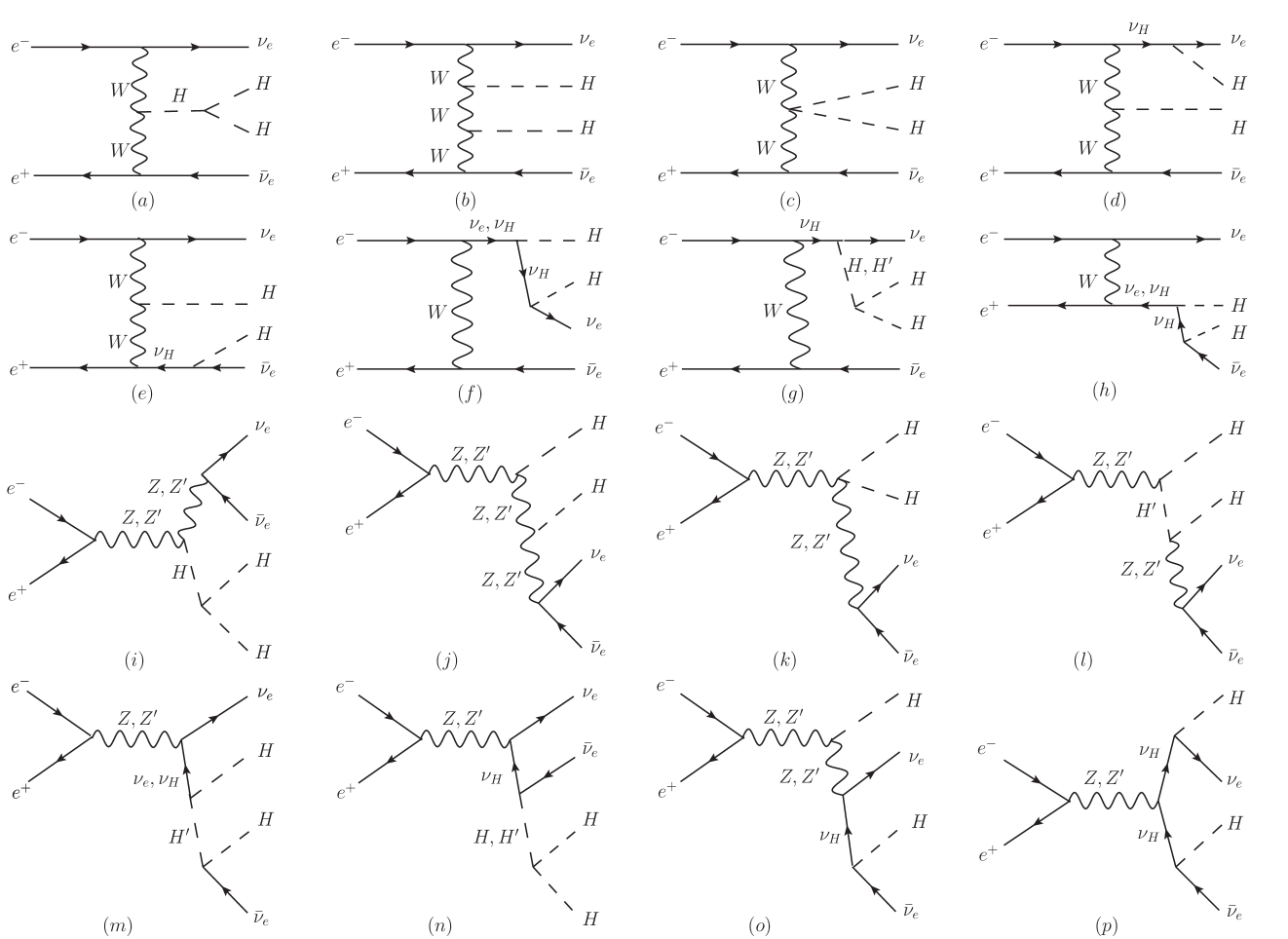
Figure 6: Lowest-order Feynman diagrams for $e^{+}e^{-}\rightarrow\nu_{e}\bar{\nu_{e}}HH$ in the $B-L$ model.

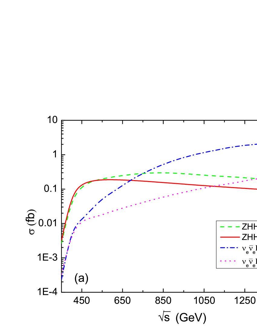
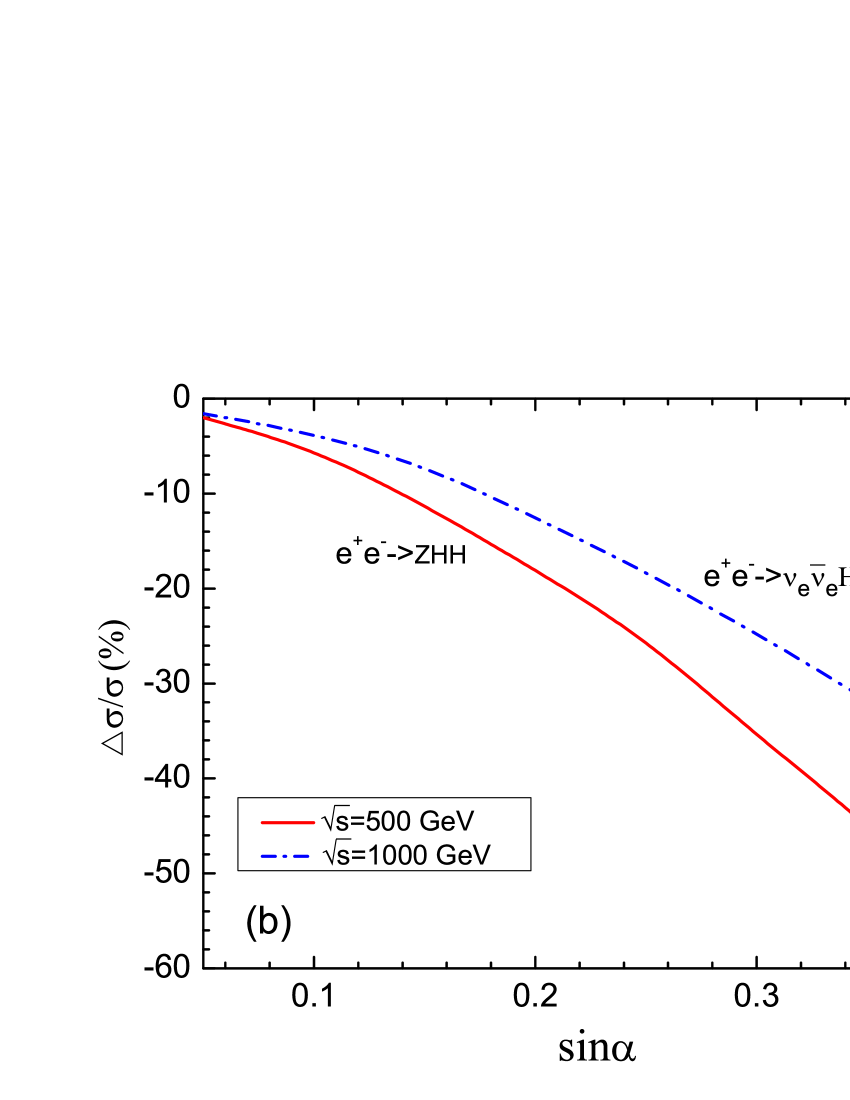
Figure 7: The production cross section $\sigma$ and the relative correction $\Delta\sigma/\sigma$ for the processes $e^{+}e^{-}\rightarrow ZHH$ and $e^{+}e^{-}\rightarrow\nu_{e}\bar{\nu_{e}}HH$ versus the c.m. energy $\sqrt{s}$ (a) and sin$\alpha$ (b) in the $B-L$ model.

In Fig.7(b), we show the relative corrections of these two double Higgs production processes versus ${\rm sin}\alpha$ for $\sqrt{s}=500,1000$ GeV with polarized beams at the ILC. We can see that the relative corrections are negative and the values become larger with the increasing of the ${\rm sin}\alpha$, which is similar to the behavior of the single Higgs production processes mentioned above. In the region of large sin$\alpha$, the $\Delta\sigma/\sigma$ of processes $ZHH$ and $\nu_{e}\bar{\nu_{e}}HH$ can reach $-56.4\%$ for $\sqrt{s}=500$ GeV and $-39.3\%$ for $\sqrt{s}=1000$ GeV, respectively. The Refs. LHC-1 ; LHC-2 ; LHC-5 ; HL-LHC-1 ; HL-LHC-2 ; HL-LHC-3 ; HL-LHC-4 ; HL-LHC-5 ; HL-LHC-6 suggest that the expected accuracy for the $HHH$ coupling could be reached 50% through $pp\rightarrow HH\rightarrow bb\gamma\gamma$ at the HL-LHC with $\mathcal{L}$=3000 fb^-1, and this accuracy may be further improved to be around 13% at the ILC with $\sqrt{s}$=1000 GeV LHC-1 ; LHC-2 ; LHC-5 ; HL-LHC-1 . By this token, the effects of the $B-L$ model might be observed through these two processes at the ILC.

IV The Higgs signal strengths in the B-L model

In order to provide more information for probing the Higgs boson processes, we give the Higgs signal strengths in the $B-L$ model. Considering the Higgs boson decay mode, the signal strengths can be defined as

$$\mu_{i}=\frac{\sigma_{B-L}\times BR(H\rightarrow i)_{B-L}}{\sigma_{SM}\times BR(H\rightarrow i)_{SM}},$$ (13)

where $i$ denotes a possible final state of the SM fermion and boson pairs.

Table 1: Expected accuracies for cross section times branching ratio measurements for the 125 GeV Higgs boson ILC-2 .

	$\Delta(\sigma\cdot BR)/(\sigma\cdot BR)$
$\mathcal{L}$ and $\sqrt{s}$	250 fb-1 at 250 GeV		500 fb-1 at 500 GeV				1000 fb-1 at 1000 GeV
$(P_{e^{-}},P_{e^{+}})$	(-0.8, +0.3)		(-0.8, +0.3)				(-0.8, +0.2)
mode	$ZH$	$\nu_{e}\bar{\nu_{e}}H$	$ZH$	$\nu_{e}\bar{\nu_{e}}H$	$t\bar{t}H$	$ZHH$	$\nu_{e}\bar{\nu_{e}}H$	$t\bar{t}H$	$\nu_{e}\bar{\nu_{e}}HH$
$H\rightarrow b\bar{b}$	$1.1\%$	$10.5\%$	$1.8\%$	$0.66\%$	$35\%$	$64\%$	$0.47\%$	$8.7\%$	$38\%$
$H\rightarrow c\bar{c}$	$7.4\%$	-	$12\%$	$6.2\%$	-	-	$7.6\%$	-	-
$H\rightarrow gg$	$9.1\%$	-	$14\%$	$4.1\%$	-	-	$3.1\%$	-	-
$H\rightarrow WW^{\ast}$	$9.1\%$	-	$9.2\%$	$2.6\%$	-	-	$3.3\%$	-	-
$H\rightarrow\tau^{+}\tau^{-}$	$4.2\%$	-	$5.4\%$	$14\%$	-	-	$3.5\%$	-	-
$H\rightarrow ZZ^{\ast}$	$19\%$	-	$25\%$	$8.2\%$	-	-	$4.4\%$	-	-
$H\rightarrow\gamma\gamma$	29-38%	-	29-38%	20-26%	-	-	7-10%	-	-

The expected accuracies for $\Delta(\sigma\cdot BR)/(\sigma\cdot BR)$ measurements for $m_{H}=125$ GeV at the ILC are shown in Table 1. Due to the $b\bar{b}$ decay mode is more easily achievable than other modes ILC-1 ; ILC-2 , we only consider this decay mode in the following section. The expected precision limits of the $b\bar{b}$ mode respectively correspond to the blue dash-dot lines in the numerical figures.

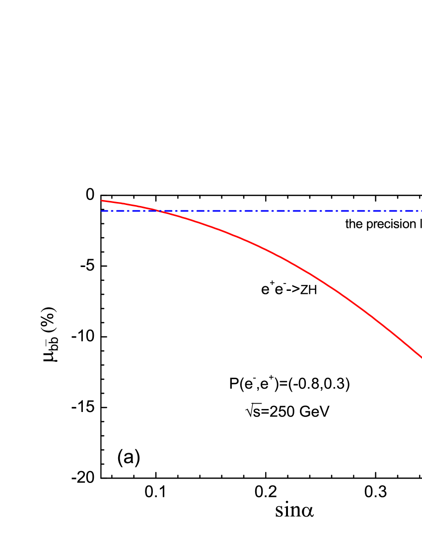
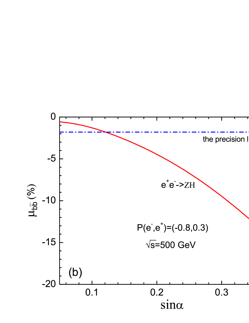
Figure 8: Higgs signal strengths $\mu_{b\bar{b}}$ for the process $e^{+}e^{-}\rightarrow ZH$ versus ${\rm sin}\alpha$ for $\sqrt{s}=250$ GeV (a) and $\sqrt{s}=500$ GeV (b) in the $B-L$ model.

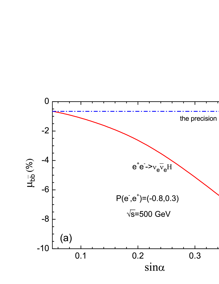
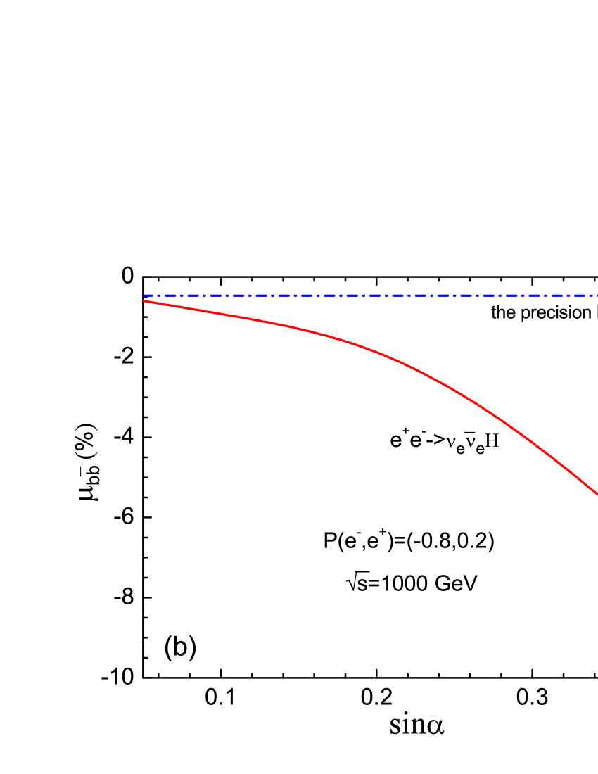
Figure 9: Higgs signal strengths $\mu_{b\bar{b}}$ for the process $e^{+}e^{-}\rightarrow\nu_{e}\bar{\nu_{e}}H$ versus ${\rm sin}\alpha$ for $\sqrt{s}=500$ GeV (a) and $\sqrt{s}=1000$ GeV (b) in the $B-L$ model.

In Fig.8, we show the dependence of the Higgs signal strengths $\mu_{b\bar{b}}$ on the parameter sin$\alpha$ for the process $e^{+}e^{-}\rightarrow ZH$ with polarized beams. From Table 1, we can see that the 1.1(1.8)% accuracy for this mode are expected at $\sqrt{s}$ = 250(500) GeV, and the contributions of the $B-L$ model might be detected by the measurement of the $b\bar{b}$ signal rate in the future ILC experiments for sin$\alpha>0.1$.

In Fig.9, we show the dependence of the Higgs signal strengths $\mu_{b\bar{b}}$ on the parameter sin$\alpha$ for the processes $e^{+}e^{-}\rightarrow\nu_{e}\bar{\nu_{{e}}}H$ with polarized beams. From Table 1, we can see that the 0.66(0.47)% accuracy for the processes $e^{+}e^{-}\rightarrow\nu_{e}\bar{\nu_{{e}}}H$ are expected at $\sqrt{s}$ = 500(1000) GeV. This accuracy is so high that almost any deviation from the SM prediction can be detected by the measurement of the $b\bar{b}$ signal rate. Conversely, the ILC measurement will give strong bound on the $B-L$ parameter if this effect can not be detected.

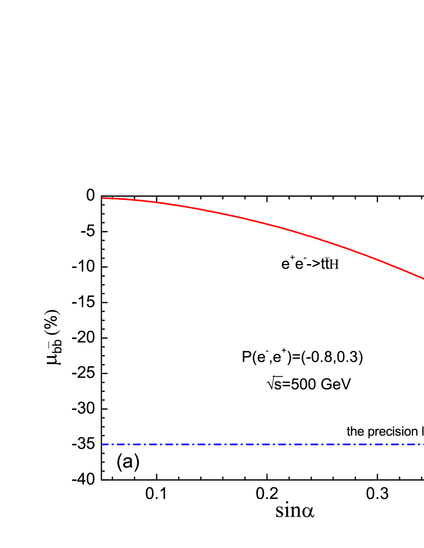
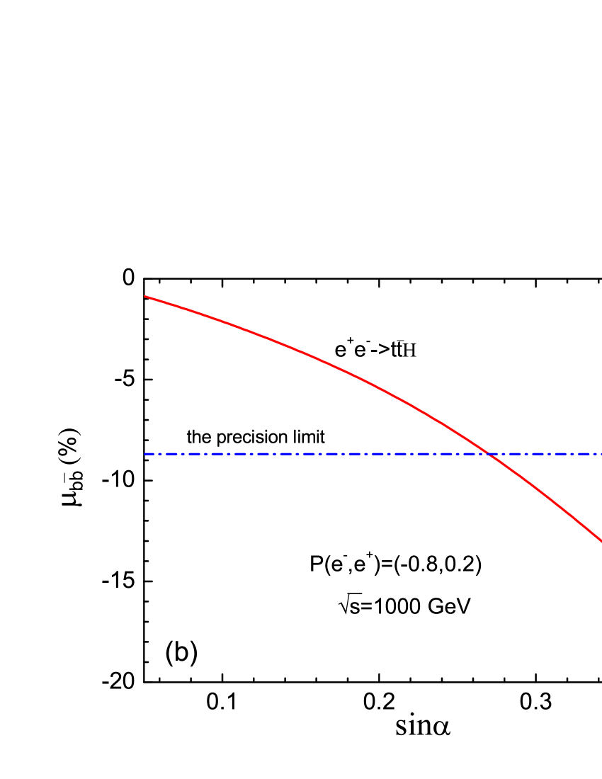
Figure 10: Higgs signal strengths $\mu_{b\bar{b}}$ for the process $e^{+}e^{-}\rightarrow t\bar{t}H$ versus ${\rm sin}\alpha$ for $\sqrt{s}=500$ GeV (a) and $\sqrt{s}=1000$ GeV (b) in the $B-L$ model.

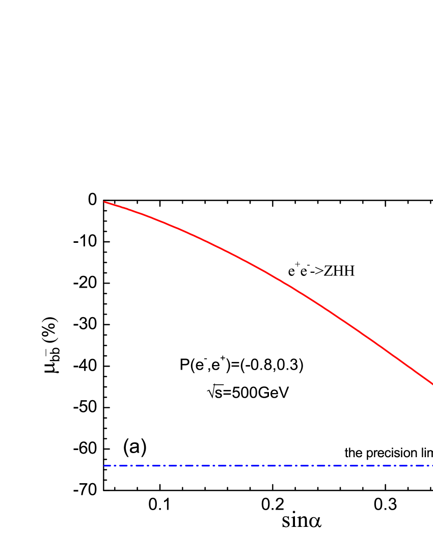
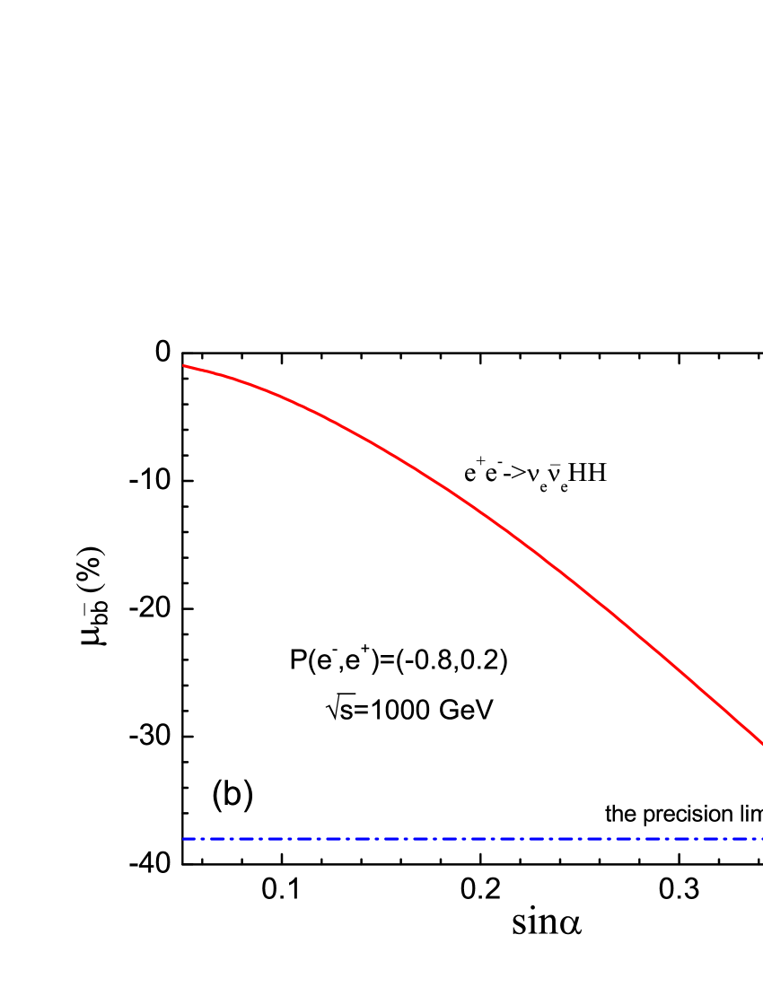
Figure 11: Higgs signal strengths $\mu_{b\bar{b}}$ for the process $e^{+}e^{-}\rightarrow ZHH$ at $\sqrt{s}=500$ GeV (a) and $e^{+}e^{-}\rightarrow\nu_{e}\bar{\nu_{e}}HH$ at $\sqrt{s}=1000$ GeV (b) versus ${\rm sin}\alpha$ in the $B-L$ model.

In Fig.10, we show the dependence of the Higgs signal strengths $\mu_{b\bar{b}}$ on the parameter sin$\alpha$ for the processes $e^{+}e^{-}\rightarrow t\bar{t}H$ with polarized beams. From Table 1, we can see that the accuracy for top Yukawa coupling is about 35% at $\sqrt{s}$ = 500 GeV, which is difficult to observe the $B-L$ effect on the process $e^{+}e^{-}\rightarrow t\bar{t}H$ via the $b\bar{b}$ channel. However, this accuracy can be improved to 8.7% at $\sqrt{s}$ = 1000 GeV so that the $B-L$ effect of this process may be detected at the high energy ILC for sin$\alpha\geq 0.3$.

In Fig.11, we show the dependence of the Higgs signal strengths $\mu_{b\bar{b}}$ on the parameter sin$\alpha$ for the double Higgs production processes $e^{+}e^{-}\rightarrow ZHH$ and $e^{+}e^{-}\rightarrow\nu_{e}\bar{\nu_{e}}HH$ with polarized beams, respectively. We can see that the Higgs signal strengths $\mu_{b\bar{b}}$ of these two processes are both below the expected precision limits so that these effects will be hard to be observed at the ILC.

V summary

Under current constraints, we investigated the single and double Higgs boson production processes $e^{+}e^{-}\rightarrow ZH$, $e^{+}e^{-}\rightarrow\nu_{e}\bar{\nu_{e}}H$, $e^{+}e^{-}\rightarrow t\bar{t}H$, $e^{+}e^{-}\rightarrow ZHH$ and $e^{+}e^{-}\rightarrow\nu_{e}\bar{\nu_{e}}HH$ in the $B-L$ model at the ILC. We calculated the production cross sections and the relative corrections with the polarized beams for $\sqrt{s}$=250 GeV, 500 GeV, 1000 GeV. We also studied the signal rates with the SM-like Higgs boson decaying to $b\bar{b}$, and performed a simulation by using the projected sensitivities given by the ILC. For the three single Higgs boson production processes, we found that the processes $e^{+}e^{-}\rightarrow ZH$ and $e^{+}e^{-}\rightarrow\nu_{e}\bar{\nu_{e}}H$ might approach the observable threshold of the ILC in the allowed parameter space. For the two double Higgs boson production processes, we found that the Higgs signal strengths $\mu_{b\bar{b}}$ of them are all out of the observed threshold of the ILC in most regions of parameter space so that the effects will be difficult to be observed at the ILC.

Appendix

Table 2: The relevant Feynman rules for single and double Higgs boson processes in the minimal $B-L$ model at the ILC.

vertices	Variational derivative of Lagrangian by fields
${H}$ - ${Z}_{\mu}$ - ${Z}_{\nu}$ -	$\frac{c_{\alpha}em_{W}}{c_{w}^{2}s_{w}}g^{\mu\nu}$
${H}$ - ${Z}_{\mu}$ - ${Z^{\prime}}_{\nu}$ -	$\frac{1}{c_{w}es_{w}}[s_{w}^{2}s_{p}s_{\alpha}c_{p}m_{W}\tilde{g}^{2}-s_{w}^{4}s_{p}c_{\alpha}c_{p}m_{W}\tilde{g}^{2}$
	$-s_{w}c_{w}c_{\alpha}em_{w}\tilde{g}+2s_{w}s_{p}^{2}c_{w}c_{\alpha}em_{w}\tilde{g}-s_{p}c_{\alpha}c_{p}e^{2}m_{w}$
	$-8s_{w}s_{\alpha}s_{p}c_{p}eg^{\prime 2}v^{\prime}+8s_{w}^{3}s_{\alpha}s_{p}c_{p}eg^{\prime 2}v^{\prime}]g^{\mu\nu}$
${H}$ - ${Z^{\prime}}_{\mu}$ - ${Z^{\prime}}_{\nu}$ -	$-8s_{\alpha}g^{\prime}_{1}{}^{2}xg^{\mu\nu}$
${H}$ - $W^{+}_{\mu}$ - $W^{-}_{\nu}$ -	$\frac{c_{\alpha}em_{W}}{s_{w}}g^{\mu\nu}$
${H^{\prime}}$ - ${Z}_{\mu}$ - ${Z}_{\nu}$ -	$\frac{em_{W}s_{\alpha}}{c_{w}^{2}s_{w}}g^{\mu\nu}$
$\bar{t}{}$    - $t{}$   - ${H}$ -	$-\frac{1}{2}\frac{c_{\alpha}em_{t}}{m_{W}s_{w}}$
$\bar{t}{}$    -$t{}$   - ${Z}_{\mu}$ -	$-\frac{1}{6}\frac{e}{c_{w}s_{w}}\gamma^{\mu}\big{(}(3-4s_{w}^{2}){(1-\gamma^{5})\over 2}-4s_{w}^{2}{(1+\gamma^{5})\over 2}\big{)}$
$\bar{t}{}$   - $t{}$   - ${Z^{\prime}}_{\mu}$ -	$-\frac{1}{3}g^{\prime}_{1}\gamma^{\mu}$
${\nu l}^{i}_{a}$ - ${\nu l}^{i}_{b}$ - ${Z}_{\mu}$ -	$\frac{1}{2}\frac{c_{ai}^{2}e}{c_{w}s_{w}}\gamma_{ac}^{\mu}\gamma_{cb}^{5}$
${\nu l}^{i}_{a}$ - ${\nu l}^{i}_{b}$ -${Z^{\prime}}_{\mu}$ -	$-(1-2s_{ai}^{2})g^{\prime}_{1}\gamma_{ac}^{\mu}\gamma_{cb}^{5}$
${\nu l}^{i}_{a}$ - ${\nu h}^{1}_{b}$ -$~{}{H}$ -	$-\frac{1}{2}\frac{1}{v^{\prime}}\big{(}(1-2s_{ai}^{2})c_{\alpha}\sqrt{2}v^{\prime}y^{\nu}_{i}\delta_{ab}+2s_{\alpha}s_{ai}c_{ai}m_{\nu_{i}}\delta_{ab}\big{)}$
${\nu l}^{i}_{a}$ - ${\nu h}^{1}_{b}$ -${H^{\prime}}$ -	$-\frac{1}{2}\frac{1}{v^{\prime}}\big{(}(1-2s_{ai}^{2})s_{\alpha}\sqrt{2}v^{\prime}y^{\nu}_{i}\delta_{ab}-2s_{ai}c_{\alpha}c_{ai}m_{\nu_{i}}\delta_{ab}\big{)}$
${H}$  - ${H}$ - ${H}$ -	$-3\frac{1}{e}\big{(}4c_{\alpha}^{3}s_{w}m_{W}\lambda_{1}-2s_{\alpha}^{3}e\lambda_{2}v^{\prime}-c_{\alpha}^{2}s_{\alpha}e\lambda_{3}v^{\prime}$
	$+2s_{w}s_{\alpha}^{2}c_{\alpha}m_{W}\lambda_{3}\big{)}$
${H}$ -  ${H}$  - ${H^{\prime}}$ -	$-\frac{1}{e}\big{(}12c_{\alpha}^{2}s_{w}s_{\alpha}m_{W}\lambda_{1}+6s_{\alpha}^{2}c_{\alpha}e\lambda_{2}v^{\prime}+(1-3s_{\alpha}^{2})c_{\alpha}e\lambda_{3}v^{\prime}$
	$-2(2-3s_{\alpha}^{2})s_{w}s_{\alpha}m_{W}\lambda_{3}\big{)}$
${H}$ - ${H}$ - $W^{+}_{\mu}$ - $W^{-}_{\nu}$ -	$\frac{1}{2}\frac{c_{\alpha}^{2}e^{2}}{s_{w}^{2}}g^{\mu\nu}$
${H}$ - ${H}$ - ${Z}_{\mu}$ - ${Z}_{\nu}$ -	$\frac{1}{2}\frac{c_{\alpha}^{2}e^{2}}{c_{w}^{2}s_{w}^{2}}g^{\mu\nu}$

Here, $e$ is the electric charge, $s_{w}$($c_{w}$) $\Rightarrow$ $\sin{\theta_{W}}$($\cos{\theta_{W}}$), $s_{\alpha}$($c_{\alpha}$) $\Rightarrow$ $\sin{\alpha}$($\cos{\alpha}$), $s_{\alpha i}$($c_{\alpha i}$) is the sinus(cosinus) of the “see-saw” mixing of the $i^{th}$ neutrino generation, $s_{p}=\frac{1}{2}{\rm sin(arcsin}(s_{n}/\sqrt{s_{n}^{2}+c_{n}^{2}}))$, $c_{p}=\sqrt{1-s_{p}^{2}}$, $s_{n}=2\tilde{g}\sqrt{(\frac{e}{s_{w}})^{2}+(\frac{e}{c_{w}})^{2}}$, $c_{n}=\tilde{g}^{2}+16g^{\prime 2}(\frac{v^{\prime}}{v})^{2}-(\frac{e}{s_{w}})^{2}-(\frac{e}{c_{w}})^{2}$.

References

- (1) ATLAS Collaboration (G. Aad et al.), Phys. Lett. B 716, 1-29 (2012).
- (2) CMS Collaboration (S. Chatrchyan et al.), Phys. Lett. B 716, 30-61 (2012).
- (3) T. Han, Z. Liu and J. Sayre, Phys. Rev. D 89, 113006 (2014).
- (4) P. Bechtle, S. Heinemeyer, O. Stal, T. Stefaniak and G. Weiglein, JHEP 1411, 039 (2014).
- (5) C. Englert, A. Freitas, M. Muhlleitner et al., J. Phys. G 41, 113001 (2014).
- (6) M. E. Peskin, arXiv:1312.4974 [hep-ph].
- (7) S. Dawson, A. Gritsan, H. Logan et al., arXiv:1310.8361 [hep-ex].
- (8) T. Behnke, J. E. Brau, B. Foster et al., arXiv:1306.6327 [acc-ph].
- (9) H. Baer, T. Barklow, K. Fujii et al., arXiv:1306.6352 [hep-ph].
- (10) D. M. Asner, T. Barklow, C. Calancha et al., arXiv:1310.0763 [hep-ph].
- (11) B. A. Kniehl, Int. J. Mod. Phys. A 17, 1457-1476 (2002).
- (12) F. Jegerlehner, O. Tarasov, Nucl. Phys. Proc. Suppl. 116, 83-87 (2003).
- (13) G. Belanger et al., Phys. Lett. B 559, 252-262 (2003).
- (14) F. Boudjema et al., Phys. Lett. B 600, 65-76 (2004).
- (15) A. Denner, S. Dittmaier, M. Roth and M. M. Weber, Phys. Lett. B 560, 196-203 (2003).
- (16) A. Denner, S. Dittmaier, M. Roth and M. M. Weber, Nucl. Phys. B 660, 289-321 (2003).
- (17) P. S. Bhupal Dev et al., Phys. Rev. Lett. 100, 051801 (2008).
- (18) H. Eberl, W. Majerotto and V. C. Spanos, Nucl. Phys. B 657, 378-396 (2003).
- (19) T. Hahn, S. Heinemeyer and G. Weiglein, Nucl. Phys. B 652, 229-258 (2003).
- (20) J. J. Cao, C. C. Han, J. Ren et al., arXiv:1410.1018 [hep-ph].
- (21) A. GutiLérrez-RodrLíguez and M. A. Hernández-Ruiz, Adv. High Energy Phys. 2015, 593898 (2015).
- (22) S. Banerjee et al., Phys. Rev. D 92, 075002 (2015).
- (23) C. -X. Yue, S. Z. Wang and D. Q. Yu, Phys. Rev. D 68, 115004 (2003).
- (24) C. -X. Yue, W. Wang, Z. J. Zong and F. Zhang, Eur. Phys. Jour. C 42, 331 (2005).
- (25) X. L. Wang, Y. -B. Liu, J. H. Chen and H. Yang, Eur. Phys. Jour. C 49, 593-597 (2007).
- (26) S. L. Hu, N. Liu, J. Ren and L. Wu, J. Phys. G 41, 125004 (2014).
- (27) N. Liu, J. Ren, L. Wu , P. W. Wu and J. M. Yang, JHEP 1404, 189 (2014).
- (28) B. F. Yang, J. Z. Han, S. H. Zhou and N. Liu, J. Phys. G 41, 075009 (2014).
- (29) S. Antusch, E. Cazzato and O. Fischer, JHEP 1604, 189 (2016).
- (30) L. Wang, W. Y. Wang, J. M, Yang and H. J. Zhang, Phys. Rev. D 75, 074006 (2007).
- (31) J. F. Shen, J. Cao and L. B. Yan, Europhys. Lett. 91, 51001 (2010).
- (32) N. Liu, S. L. Hu, B. F. Yang and J. Z. Han, JHEP 1501, 008 (2015).
- (33) B. F. Yang, Z. Y. Liu, N. Liu and J. Z. Han, Eur. Phys. Jour. C 74, 3203 (2014).
- (34) B. F. Yang, J. Z. Han and N. Liu, JHEP 1504, 148 (2015).
- (35) L. Wu, JHEP 1502, 061 (2015).
- (36) Y.-B. Liu and Z.-J. Xiao, J. Phys. G 42, 065005 (2015).
- (37) J. Z. Han, S. F. Li, B. F. Yan and N. Liu, Nucl. Phys. B 896, 200-211 (2015).
- (38) S. Khalil, J. Phys. G 35, 055001 (2008).
- (39) L. Basso, arXiv:1106.4462.
- (40) W. Emam and S. Khalil, Eur. Phys. Jour. C 52, 625-633 (2007).
- (41) L. Basso, A. Belyaev, S. Moretti and C. H. Shepherd-Themistocleous, Phys. Rev. D 80, 055030 (2009).
- (42) L. Basso, A. Belyaev, S. Moretti and G. M. Pruna, JHEP 0910, 006 (2009).
- (43) P. Fileviez Perez, T. Han, and T. Li, Phys. Rev. D 80, 073015 (2009).
- (44) L. Basso, S. Moretti, and G. M. Pruna, Eur. Phys. Jour. C 71, 1724 (2011).
- (45) L. Basso, S. Moretti and G. M. Pruna, Phys. Rev. D 83, 055014 (2011).
- (46) G. M. Pruna, arXiv:1106.4691 [hep-ph].
- (47) C. Englert, T. Plehn, D. Zerwas and P. M. Zerwas, Phys. Lett. B 703, 298-305 (2011).
- (48) V. V. Khoze and G. Ro, JHEP 1310, 075 (2013).
- (49) J. Hernández López and J. Orduz-Ducuara, J. Phys. Conf. Ser. 468, 012012 (2013).
- (50) R. Marshak and R. N. Mohapatra, Phys. Lett. B 91, 222-224 (1980).
- (51) R. N. Mohapatra and R. Marshak, Phys. Rev. Lett. 44, 1316-1319 (1980).
- (52) C. Wetterich, Nucl. Phys. B 187, 343-375 (1981).
- (53) A. Masiero, J. Nieves and T. Yanagida, Phys. Lett. B 116, 11-15 (1982).
- (54) R. N. Mohapatra and G. Senjanovic, Phys. Rev. D 27, 254 (1983).
- (55) G. Cacciapaglia, C. Csaki, G. Marandella and A. Strumia, Phys. Rev. D 74, 033011 (2006).
- (56) Particle Data Group collaboration (K. A. Olive et al.), Chin. Phys. C 38, 090001 (2014).
- (57) S. Banerjee, M. Mitra and M. Spannowsky, Phys. Rev. D 92, 055013 (2015).
- (58) A. Belyaev, N. D. Christensen and A. Pukhov, Comput. Phys. Commun. 184, 1729 (2013).
- (59) G. Moortgat-Pick, T. Abe, G. Alexander et al., Phys. Rept. 460, 131 (2008).
- (60) J. J. Cao, Z. X. Heng, L. Wu and J. M. Yang, Phys. Rev. D 81, 014016 (2010).
- (61) A. Denner, J. Kublbeck, R. Mertig and M. Bohm, Z. Phys. C 56, 261 (1992).
- (62) C. Englert and M. McCullough, JHEP 1307, 168 (2013).
- (63) M. E. Peskin, arXiv:1312.4974 [hep-ph].
- (64) F. Goertz, A. Papaefstathiou, L. L. Yang and J. Zurita, JHEP 1306, 016 (2013).
- (65) R. S. Gupta, H. Rzehak and J. D. Wells, Phys. Rev. D 88, 055024 (2013).
- (66) A. J. Barr, M. J. Dolan, C. Englert and M. Spannowsky, Phys. Lett. B 728, 308-313 (2014).
- (67) V. Barger, L. L. Everett, C. B. Jackson and G. Shaughnessy, Phys. Lett. B 728, 433 (2014).
- (68) D. E. F. de Lima, A. Papaefstathiou and M. Spannowsky, JHEP 1408, 030 (2014).