Non-standard charged Higgs decay at the LHC in Next-to-Minimal Supersymmetric Standard Model

Abstract

We consider next-to-minimal supersymmetric standard model (NMSSM) which has a gauge singlet superfield. In the scale invariant superpotential we do not have the mass terms and the whole Lagrangian has an additional $Z_{3}$ symmetry. This model can have light scalar and/or pseudoscalar allowed by the recent data from LHC and the old data from LEP. We investigate the situation where a relatively light charged Higgs can decay to such a singlet-like pseudoscalar and a $W^{\pm}$ boson giving rise to a final state containing $\tau$ and/or $b$-jets and lepton(s). Such decays evade the recent bounds on charged Higgs from the LHC, and according to our PYTHIA-FastJet based simulation can be probed with 10 fb^-1 at the LHC center of mass energy of 13 and 14 TeV.

1 Introduction

The recent discovery of the Higgs boson at the LHC, both by ATLAS ATLAS and CMS CMS ; CMS2 is the so-called ‘last key stone’ of the Standard Model (SM). The observation of the Higgs boson with mass around $125$ GeV has reached around or more than $5\sigma$ level for $WW^{*}$, $ZZ^{*}$ and $\gamma\gamma$ modes so far ATLAS ; CMS ; CMS2 . The fermionic modes are yet to reach the discovery level. Although this Higgs boson is believed to be responsible for the electroweak symmetry breaking (EWSB) mechanism in the SM, precise measurements of its properties (couplings etc.) are still required to prove this statement. However, the situation in the Higgs sector still remains open since various new physics models can explain the presence of the newly discovered Higgs boson.

Any scalar mass not protected by any symmetry leads to the so-called hierarchy problem hierarchy (i.e. problems in the stability of mass against large quantum corrections). One of the most popular solution to this problem is to extend the SM in a minimally supersymmetric way (called minimal supersymmetric standard model or MSSM). However, in the CP-conserving sector of the theory the lightest Higgs mass is bounded from above by the $Z$ mass ($m_{h_{1}}\lesssim M_{Z}$). LEP experiments searched for the supersymmetric Higgs and put a direct lower bound on its mass to around $93$ GeV LEPb . Thus to satisfy both the LEP bound and LHC discovery one needs to calculate Higgs boson mass at one-loop. All the particles that interact with the Higgs boson, contribute to its mass via virtual corrections and the dominant ones come from the third generation quark and squark sectors due to their large Yukawa coupling with the Higgs. In order to achieve $125$ GeV Higgs mass, loop corrections are required to be sizeable in MSSM. This, in turn, puts strong constraint on the SUSY mass scale. For the most constrained SUSY scenarios like mSUGRA, the required mass scale is above a few TeV cMSSMb . On the other hand, for the phenomenological SUSY scenarios, like pMSSM, one either needs large SUSY mass scale or larger mass splitting between the two scalar tops (stop squarks) cMSSM . This, in a sense, brings back the fine-tuning problem.

Extension of MSSM in a minimal way by adding a singlet scalar superfield is a natural remedy to the problem. This scenario is known as next-to-minimal supersymmetric standard model (NMSSM)Ellwanger:2009dp in which a singlet scalar contributes to the Higgs mass at the tree-level as well as at the loop-level. This naturally lifts the Higgs mass to the desired range of around $125$ GeV without the requirement of a high mass scale.

NMSSM is originally motivated by solving the $\mu$-problem in MSSM. The $\mu$-term ($\mu H_{u}H_{d}$) is the supersymmetric version of the Higgs mass term in SM and provides the mass term for the higgsino (the fermionic superpartner of Higgs). It also contributes to the $Z$ boson mass which is certainly at the electroweak scale. Therefore, one expects it to be of the order of electroweak scale ($\approx 10^{2}$ GeV to $1$ TeV). On the other hand, this term is supersymmetry conserving and it could be present at any scale, assuming practically any value. This leads to the famous $\mu$-problem in MSSM. Introduction of a singlet scalar superfield which couples to both the Higgs doublets can generate the $\mu$-term dynamically when the singlet field gets a vacuum expectation value (vev) nmssm . Still one can not make the $\mu$-term vanish arbitrarily unless some symmetry prohibits it. Generally, a discrete symmetry, named $Z_{3}$ symmetry (which corresponds to multiplication of all components of the chiral superfields by a phase $e^{2\pi i/3}$) is imposed on the NMSSM superpotential. This discrete symmetry forbids any bilinear term in chiral superfields, thereby, forcing the $\mu$-term to vanish. In this work we consider a $Z_{3}$ invariant NMSSM model. In addition, we can find a light pseudoscalar as a pseudo-Nambu-Goldstone boson (pNGB) in such a scenario. LEP searched for the Higgs bosons $h_{1}$ and $a_{1}$ via $e^{+}e^{-}\to Zh_{1}$ and $e^{+}e^{-}\to a_{1}h_{1}$ (in models with multiple Higgs bosons) and their fermionic decay modes, i.e. $h_{1}/a_{1}\to b\bar{b},\tau\bar{\tau}$ and $Z\to\ell\bar{\ell}$. Such light pNGB or otherwise light scalars (both CP even and odd) when mostly singlet couple to the fermions and gauge bosons only via the mixing with the doublet type Higgs bosons, and they can evade the LEP bounds LEPb . The singlet type light pseudoscalar is consistent with LHC data. Even if it is not directly produced at the collider, indirect bounds still exist on such hidden (often termed as “buried”) state from Higgs data at the LHC.

Apart from the decay of the discovered Higgs into the hidden scalar/pseudoscalar, the decays of other possible heavy Higgses can also be interesting. Among them the charged Higgs is very special as it would straightaway prove the existence of another Higgs doublet or, simpler, an extended Higgs sector. The masses of the other Higgs bosons in MSSM ($h_{2}$, $a$, $h^{\pm}$) are closely related to each other. For example, the masses of the CP-odd Higgs and charged Higgs bosons are given by the relation $m_{h^{\pm}}^{2}=m^{2}_{a}+m_{W^{\pm}}^{2}$ at tree-level. As a result, the decay $h^{\pm}\rightarrow aW^{\pm}$ is not typically possible. Even with loop corrections, this degeneracy is very unlikely to be broken. The additional Higgs singlet can play important role here to lift such degeneracy between the charged Higgs and the CP-odd Higgs. This means that NMSSM has one more CP-odd and one extra CP-even Higgs states compared to MSSM. The two CP-odd states mix among each other to give mass eigenstates, and thereby altering the mass relation. Therefore, the lightest CP-odd state ($a_{1}$) may become much lighter than the charged Higgs boson thus allowing the decay $h^{\pm}\rightarrow a_{1}W^{\pm}$. But kinematics, although an important factor, is not all. The charged Higgs, as we know, is mostly doublet-type. On the other hand, the lightest pseudoscalar has to have significant singlet component in order to avoid existing collider bounds. Hence, the coupling $h^{\pm}-a_{1}-W^{\pm}$ vanishes unless $a_{1}$ has got some doublet contribution via mixing.

The charged Higgs phenomenology is often considered by comparing its mass to top quark. The light charged Higgs scenario corresponds to $m_{t}>m_{h^{\pm}}$ and the rest is considered the heavy charged Higgs region. In the first case, the main production process of charged Higgs comes from $pp\rightarrow t\bar{t}$ with top decaying to $bh^{+}$. In the same region, the primary decay modes of the charged Higgs are $\tau\nu$ and $c\bar{s}$ (+ their h.c states). For a charged Higgs heavier than $m_{t}$, the primary production channel is $pp\rightarrow th^{\pm}$ and/or $tbh^{\pm}$ Bawa:1989pc ; Datta:2001qs , while the dominant decay mode of $h^{\pm}$ becomes $t\bar{b}$ (+ h.c). However, this region is overflowed by the SM processes $ttbb$ and $ttZ$ which are difficult to control Gunion:1993sv .

In this work, we are interested in studying the phenomenology of a relatively light charged Higgs (of mass just above $m_{t}$) scenario in the framework of NMSSM. We look for a hidden pseudoscalar via the search of the charged Higgs boson. In particular, our intention is to establish a probe for the charged Higgs boson decaying into a $W^{\pm}$ and a light singlet-like pesudoscalar which is otherwise difficult to produce at the LHC. Studies related to a light scalar/pseudoscalar have been discussed by many authors NMSSMps . If these hidden scalars/pseudoscalars have masses $\leq m_{h_{125}}/2$, they can be explored by the decay channel $h_{125}\to h_{1}h_{1}/a_{1}a_{1}$. On the other hand, when the masses are $>m_{h_{125}}/2$, the decay channel is no more kinematically allowed. In that case a light charged Higgs decaying to $a_{1}/h_{1}W^{\pm}$ may be the next possible option to look for.

For $m_{h^{\pm}}>m_{t}$, $bg\rightarrow th^{+}$ is the best channel to produce charged Higgses. We focus on a rather non-standard decay modes of the charged Higgs: $a_{1}/h_{1}W^{\pm}$, where the hidden scalars further decay into $b$ and/or $\tau$ pairs. We carefully look for different final states based on these non-standard decay modes and try to probe such possibilities. Charged Higgs decays to $a_{1}/h_{1}W^{\pm}$ have previously been considered in the literature Rathsman:2012dp ; chargedhiggs-pheno . Particularly, the authors in Rathsman:2012dp consider a similar scenario with light charged Higgs decaying to $a_{1}W^{\pm}$ in NMSSM. They take the usual approach to produce a $h^{\pm}$ via $t\bar{t}$ production (with one of top quark decaying to $h^{+}$ and a bottom) and keep their focus on the region of parameter space where the $a_{1}$ mass is above the $b\bar{b}$ threshold but still close to it so that the two b-quarks fragment into a single $b\bar{b}$-jet.

We organise our paper as follows. In Section 2 we give a brief introduction to the model. In Section 3 we scan the parameter space considering various theoretical and experimental bounds and select some benchmark points in Section 4. We perform the collider simulation and present our results in Section 5. Finally we conclude in Section 6.

2 The Model

In NMSSM, an $SU(2)_{L}\otimes U(1)_{Y}$ singlet complex scalar field $S$ is added to the MSSM Higgs sector. The extra singlet couples only to the MSSM Higgs doublet. The superpotential contains a new singlet interacting with the Higgs doublets along with the well-known Yukawa interactions of the up and down-type Higgs with the fermions as in the superpotential in MSSM. Other dimensionful couplings are forbidden by the imposition of the $Z_{3}$ symmetry on the superpotential which is given as

$$W_{NMSSM}=W_{MSSM}^{\mu=0}+\lambda_{S}SH_{u}\cdot H_{d}+\frac{1}{3}\kappa S^{3}.$$ (1)

The dot product denotes the usual $SU(2)_{L}$ product: $H_{u}\cdot H_{d}=H_{u}^{\alpha}\epsilon_{\alpha\beta}H_{d}^{\beta}$ with $\epsilon$ being the anti-symmetric matrix with elements off-diag$(1,-1)$. Note that the bilinear $\mu$-term is generated dynamically once the singlet acquires a vev which breaks the $Z_{3}$ symmetry. The effective term $\mu_{\text{eff}}=\lambda\langle S\rangle$ is naturally of the order of electroweak scale thus solving the supersymmetric $\mu$-problem.

The tree level scalar potential is given by Ellwanger:2009dp

$$\begin{split}V={}&\left(m_{H_{u}}^{2}+\lambda^{2}|S|^{2}\right)H_{u}^{2}+\left(m^{2}_{H_{d}}+\lambda^{2}|S|^{2}\right)H_{d}^{2}+|\lambda H_{u}\cdot H_{d}+\kappa S^{2}|^{2}\\ &+\frac{g^{\prime 2}}{8}\left(H_{u}^{2}-H_{d}^{2}\right)^{2}+\frac{g^{2}}{8}\Big{[}\left(H_{u}^{2}+H_{d}^{2}\right)^{2}-4|H_{u}\cdot H_{d}|^{2}\Big{]}\\ &+m_{S}^{2}|S|^{2}+\Big{[}\lambda A_{\lambda}SH_{u}\cdot H_{d}+\frac{1}{3}\kappa A_{\kappa}S^{3}+h.c.\Big{]},\end{split}$$ (2)

where $g^{{}^{\prime}}$ and $g$ are the $U(1)_{Y}$ and $SU(2)_{L}$ coupling constants, respectively. $m_{H_{u}}^{2}$, $m_{H_{d}}^{2}$, $m_{S}^{2}$, $A_{\kappa}$ and $A_{\lambda}$ are the soft breaking parameters. We also denote the vev of $H_{u}$, $H_{d}$ and $S$ by $v_{u}$, $v_{d}$ and $v_{s}$, respectively, with the definition $\tan\beta=v_{u}/v_{d}$. However, $M_{Z}$ and $\tan\beta$ define $v_{u}$ and $v_{d}$. Thus at the tree-level, the Higgs sector in NMSSM has the following nine parameters:

$$\lambda,\leavevmode\nobreak\ \kappa,\leavevmode\nobreak\ \tan\beta,\leavevmode\nobreak\ \mu_{\text{eff}},\leavevmode\nobreak\ A_{\lambda},\leavevmode\nobreak\ A_{\kappa},\leavevmode\nobreak\ m_{H_{u}}^{2},\leavevmode\nobreak\ m_{H_{d}}^{2},\leavevmode\nobreak\ m_{S}^{2}.$$

Three minimization conditions corresponding to three scalar superfields in $V$ can fix any three of the parameters. Usually the soft breaking mass parameters $m_{H_{u}}^{2}$, $m_{H_{d}}^{2}$, $m_{S}^{2}$ are solved, which leaves six independent parameters. Out of the ten real degrees of freedom in the fields, three have been used to give masses to the weak gauge bosons after electroweak symmetry breaking. The other seven become the physical Higgs states with three CP even ($h^{\prime}_{1}$, $h^{\prime}_{2}$, $h^{\prime}_{3}$ with any one being the $h_{125}$), two CP odd states ($a^{\prime}_{1}$, $a^{\prime}_{2}$) and two charged Higgs states ($h^{\pm}$). The neutral CP even Higgs states are given as

$$h^{\prime}_{1} =\sqrt{2}\left(\left(Re\leavevmode\nobreak\ H_{d}^{0}-v_{d}\right)\cos\beta-\left(Re\leavevmode\nobreak\ H_{u}^{0}-v_{u}\right)\sin\beta\right),$$

$$h^{\prime}_{2} =\sqrt{2}\left(\left(Re\leavevmode\nobreak\ H_{d}^{0}-v_{d}\right)\sin\beta+\left(Re\leavevmode\nobreak\ H_{u}^{0}-v_{u}\right)\cos\beta\right),$$ (3)

$$h^{\prime}_{3} =\sqrt{2}\left(Re\leavevmode\nobreak\ S-v_{s}\right).$$

The mass matrix may still not be diagonal with these rotations. After diagonalization of the mass matrix, three mass eigenstates, conventionally listed in the order of increasing mass as $h_{1}$, $h_{2}$, $h_{3}$ for CP-even and $a_{1}$, $a_{2}$ for CP-odd, are mixtures of the gauge (weak) eigenstates. $h_{1}$ usually behaves closely like the scalar discovered at the LHC. Similarly, the neutral CP odd Higgses and charged Higgs states can be written as,

$$a_{1} =\sqrt{2}\left(\left(Im\leavevmode\nobreak\ H_{d}^{0}\right)\sin\beta+\left(Im\leavevmode\nobreak\ H_{u}^{0}\right)\cos\beta\right)$$

$$a_{2} =\sqrt{2}\left(Im\leavevmode\nobreak\ S\right),$$ (4)

and

$$h^{\pm}=H_{d}^{\pm}\sin\beta+H_{u}^{\pm}\cos\beta.$$ (5)

Charged Higgs states are always purely $SU(2)_{L}$ doublet states as in MSSM. The compositions of the CP even and odd Higgs states depend on the parameters. Particularly, $\lambda$ is the main parameter which infuses singlet mixing in the CP even and odd Higgses.

3 Parameter space scan

We scan the NMSSM parameter space using the publicly available code NMSSMTools v4.7.0 nmssmtools . We focus only on the Higgs sector and try to achieve a light pseudoscalar and a relatively light charged Higgs with mass just above the top mass ($\approx 200-250$ GeV) satisfying the LHC Higgs results. We consider the parameter region where BR($h^{\pm}\to W^{\pm}a_{1}$) is significant. Usually the BR($h^{\pm}\to W^{\pm}a_{1}$) is close to other branching ratios, like BR($h^{\pm}\to t\bar{b}$, $\tau\nu$).
Here we do not vary the soft mass parameters in the stop sector in order to avoid complicated parameter dependence, but the loop corrections in Higgs mass arising from the third generation squarks have been taken into account. We have fixed values for the other slepton and squark masses. Soft SUSY breaking gaugino masses are also held to a constant value as they are barely connected to the Higgs sector. Though, their values are important while considering decays. The soft-breaking terms are as follows:

$$M_{1}=100\leavevmode\nobreak\ \text{GeV,}\leavevmode\nobreak\ \leavevmode\nobreak\ M_{2}=200\leavevmode\nobreak\ \text{GeV,}\leavevmode\nobreak\ \leavevmode\nobreak\ M_{3}=1.5\leavevmode\nobreak\ \text{TeV,}$$

$$M_{L_{1,2}}=500\leavevmode\nobreak\ \text{GeV}=M_{E_{1,2}}\text{,}\leavevmode\nobreak\ \leavevmode\nobreak\ M_{L_{3}}=500\leavevmode\nobreak\ \text{GeV}=M_{E_{3}},$$

$$M_{Q_{1,2}}=1.0\leavevmode\nobreak\ \text{TeV}=M_{{U,D_{1,2}}},$$

$$M_{Q_{3}}=700\leavevmode\nobreak\ \text{GeV,}\leavevmode\nobreak\ M_{U_{3}}=900\leavevmode\nobreak\ \text{GeV,}\leavevmode\nobreak\ M_{D_{3}}=800\leavevmode\nobreak\ \text{GeV},$$

$$A_{b,\tau}=100\leavevmode\nobreak\ \text{GeV},$$

where $M_{i=1,2,3}$ are the three gaugino masses, $M_{L},M_{E}$ are the doublet and singlet slepton masses, $M_{Q},M_{U},M_{D}$ are the doublet and singlet type squark masses where $i=1,2,3$ stands for three generations. $A_{b,\tau}$ are trilinear couplings for bottom and tau.

Since our primary goal is to study the Higgs sector, particularly the charged Higgs, we scan over the following parameter region ($\mu,\,M_{A},\,A_{\kappa},\,A_{t}$ are in GeV):

$$2.0\leavevmode\nobreak\ \leavevmode\nobreak\ \leavevmode\nobreak\ \leq \leavevmode\nobreak\ \tan\beta \leq\leavevmode\nobreak\ \leavevmode\nobreak\ \leavevmode\nobreak\ 40.0$$

$$-1000.0\leavevmode\nobreak\ \leavevmode\nobreak\ \leavevmode\nobreak\ \leq \mu \leq\leavevmode\nobreak\ \leavevmode\nobreak\ \leavevmode\nobreak\ 1000.0$$

$$0.01\leavevmode\nobreak\ \leavevmode\nobreak\ \leavevmode\nobreak\ \leq \lambda,\kappa \leq\leavevmode\nobreak\ \leavevmode\nobreak\ \leavevmode\nobreak\ 1.0$$

$$0\leavevmode\nobreak\ \leavevmode\nobreak\ \leavevmode\nobreak\ \leq M_{A} \leq\leavevmode\nobreak\ \leavevmode\nobreak\ \leavevmode\nobreak\ 400.0$$

$$-1000.0\leavevmode\nobreak\ \leavevmode\nobreak\ \leavevmode\nobreak\ \leq A_{\kappa} \leq\leavevmode\nobreak\ \leavevmode\nobreak\ \leavevmode\nobreak\ 1000.0$$

$$-2000.0\leavevmode\nobreak\ \leavevmode\nobreak\ \leavevmode\nobreak\ \leq A_{t} \leq\leavevmode\nobreak\ \leavevmode\nobreak\ \leavevmode\nobreak\ 2000.0$$ (6)

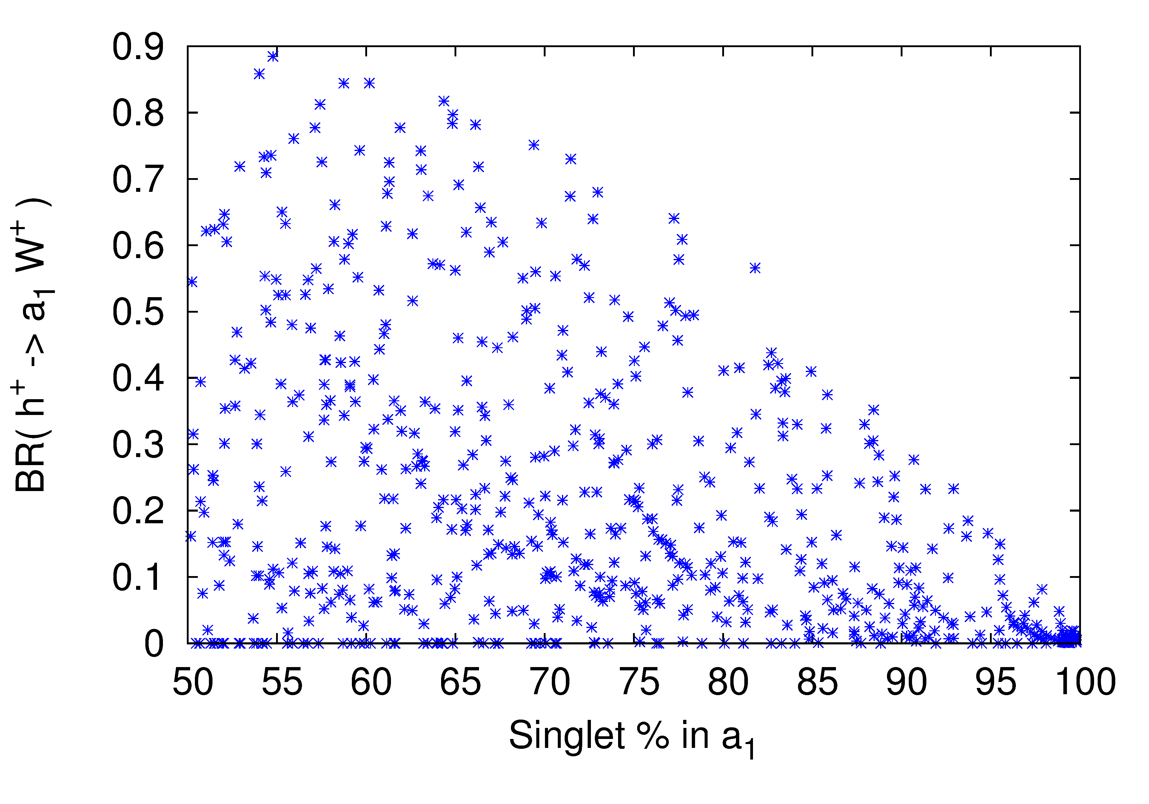
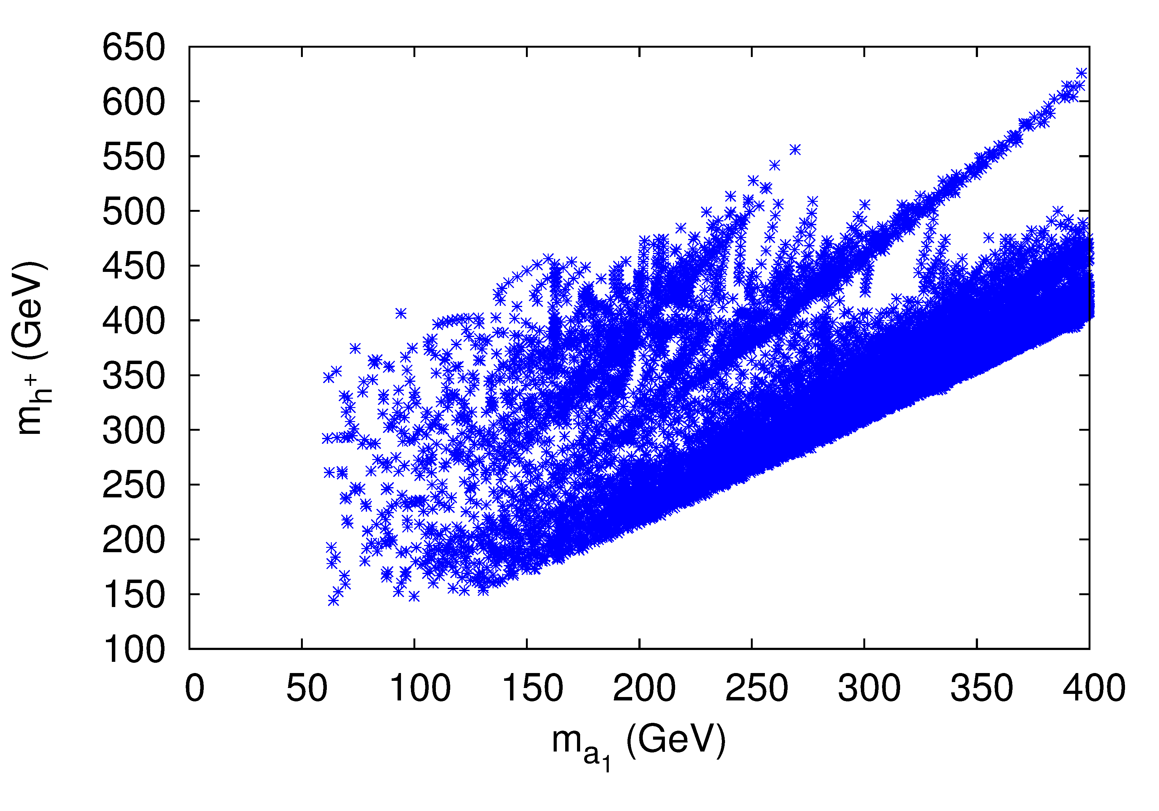
Figure 1: Left: Singlet percentage in $a_{1}$ against BR($h^{\pm}\rightarrow a_{1}W^{\pm}$). Right: Mass correlation between lightest pseudoscalar and charged Higgs.

The SUSY scale is fixed at $M_{SUSY}$ = 1 TeV. We demand that the lightest Higgs, $h_{1}$, lies within 122-128 GeV. We also require the lighter chargino mass to be greater than 105 GeV to avoid the LEP bound from chargino pair production chargino .

Left panel of Fig. 1 shows the variation of $h^{\pm}\rightarrow a_{1}W^{\pm}$ branching ratio with percentage of singlet component in the lightest pseudoscalar $a_{1}$. As mentioned in the introduction, the lightest pseudoscalar must be singlet-like to evade the LEP bound. On the other hand, $h^{\pm}$ is only doublet-type. Therefore to have the desired decay mode, one must have enough doublet component in $a_{1}$ via mixing. When $a_{1}$ becomes a pure singlet, the branching ratio goes to 0. The right plot is the correlation between masses of $a_{1}$ and $h^{\pm}$. We notice the diagonal behaviour which is clearly the MSSM limit. These two figures together give us an idea about the dynamics (i.e. coupling) and the kinematics between charged Higgs and the lightest pseudoscalar to maximize the corresponding decay channel.

In Fig. 2 we show charged Higgs branching fractions in various important decay channels. As we can see, $\tau\nu$ channel is dominant for the lightest charged Higgs masses. Once $m_{h^{+}}$ hits the top threshold, the $t\bar{b}$ channel becomes the dominant decay mode and $\tau\nu$ mode remains within 10% for the rest of the region. $W^{\pm}h_{1}$ also remains substantial in the desired charged Higgs mass range of $\approx 200-250$ GeV. Branching ratio for charged Higgs decaying to $W^{\pm}a_{1}$ can be quite large ($\sim$ 60-70%) for light $h^{\pm}$. As mass increases, the $t\bar{b}$ decay mode becomes significant. Interesting to note that in the first three plots starting from top-left, the masses of the decay products are known. Still, we see the branching ratios to be varying even for fixed mass of the parent particle. This is simply because most of the couplings depend on $\tan\beta$ (or, $\cot\beta$) and the mixing angle in the Higgs sector. Variation in relevant parameters keep the couplings changing. On the other hand, $a_{1}$ mass and its coupling in the bottom-right plot is varying. The scatter plots in Fig. 2 show how the charged Higgs branching ratios to various channels vary over its mass, although the mass of the charged Higgs is fixed.

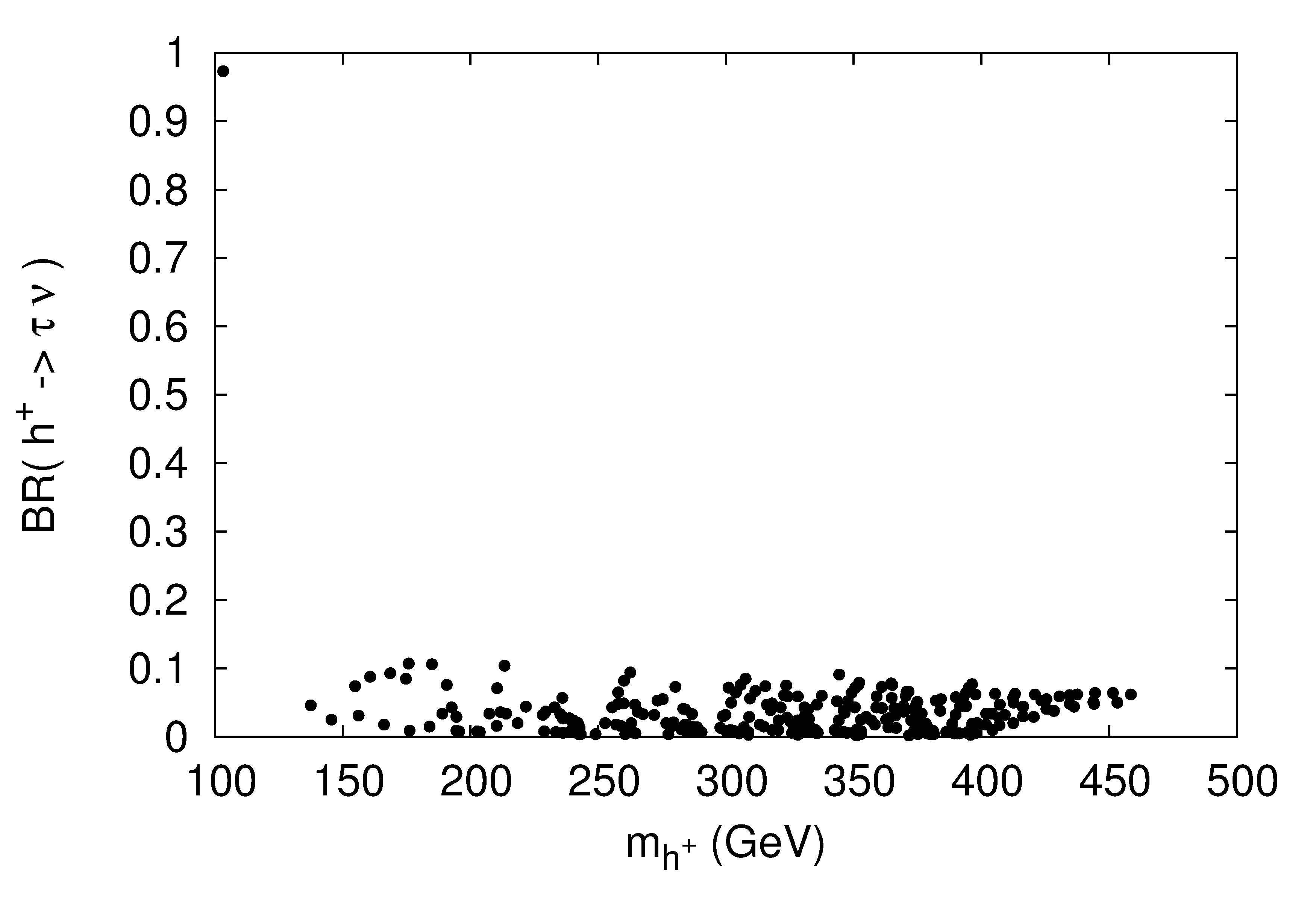
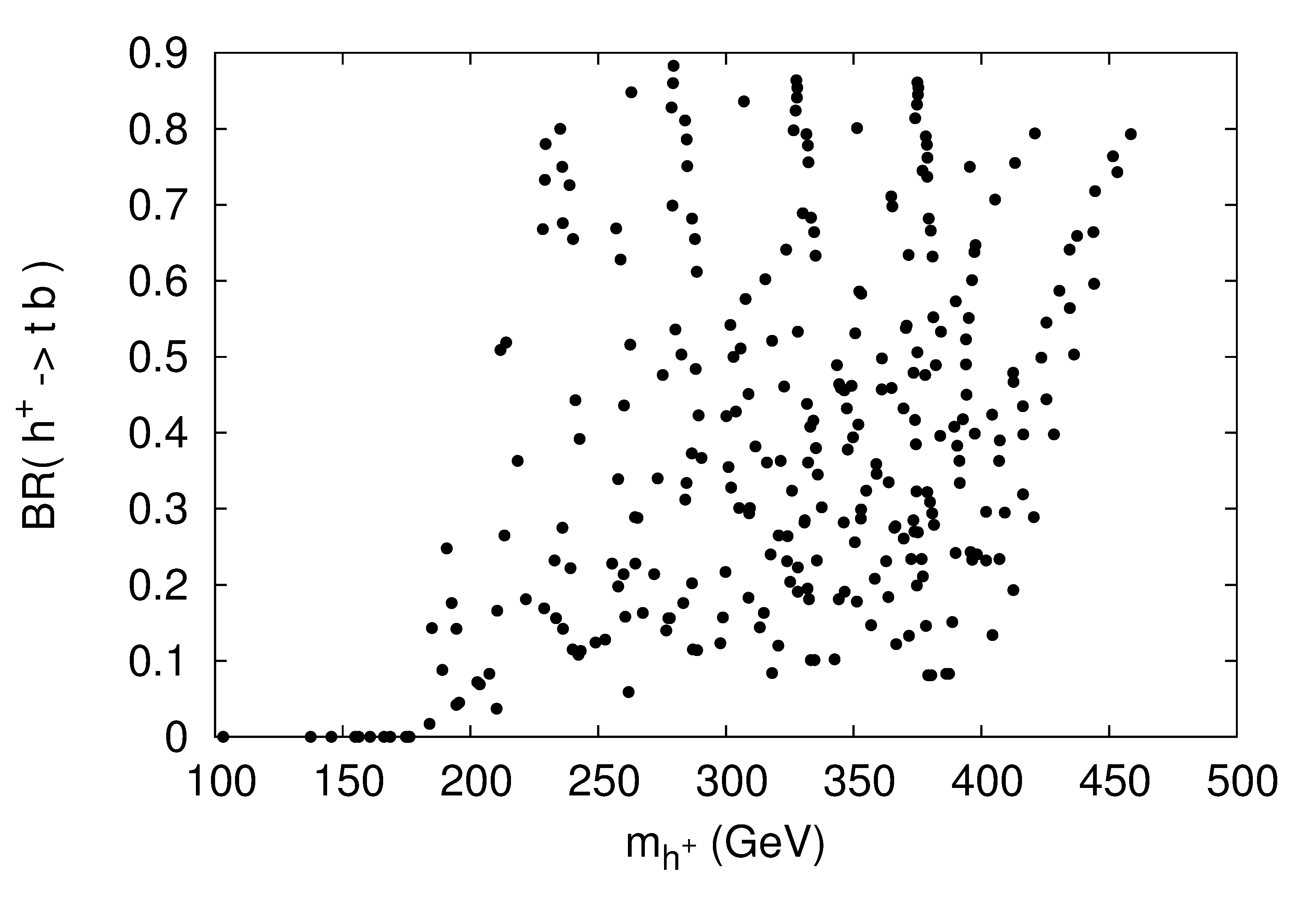
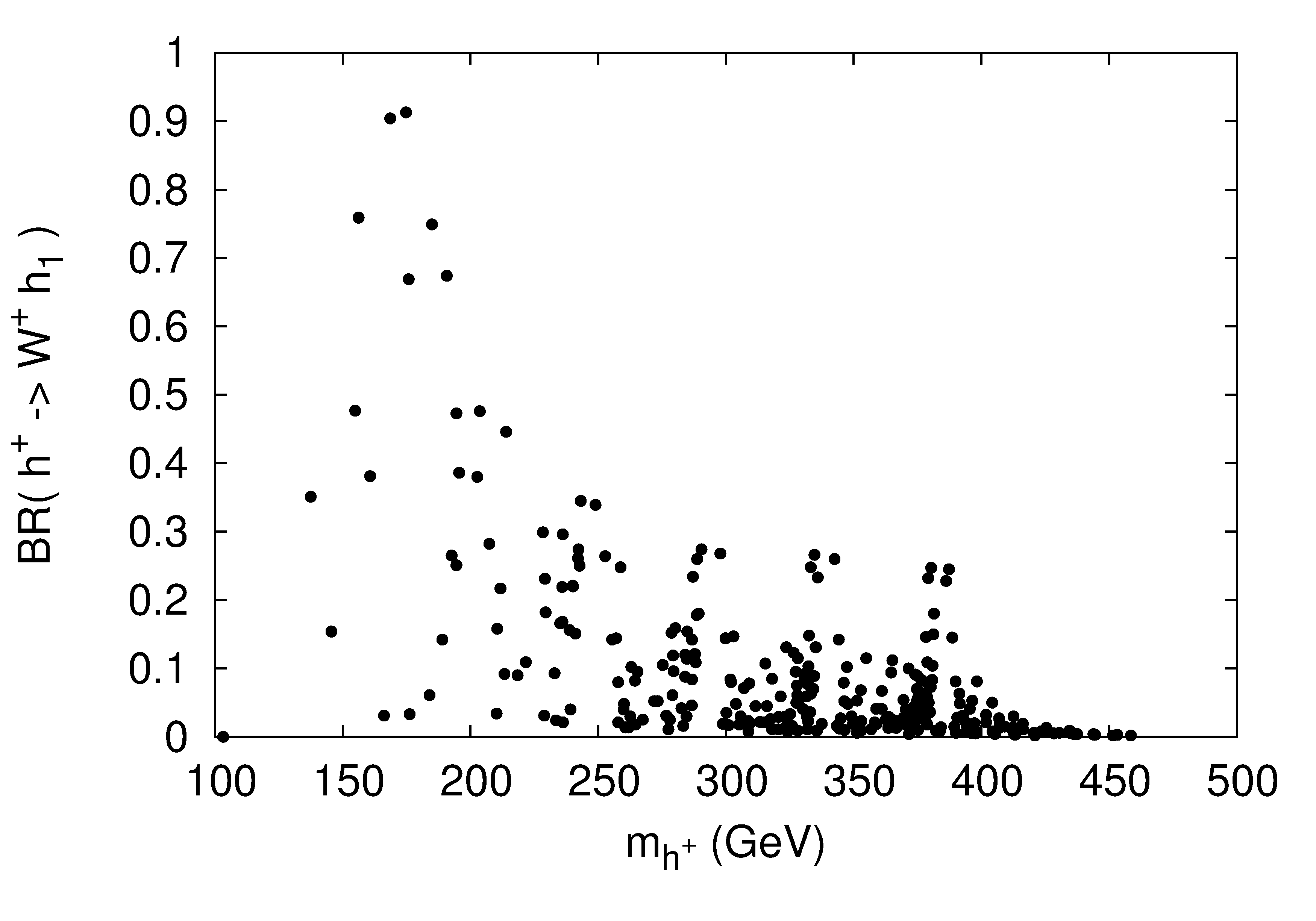
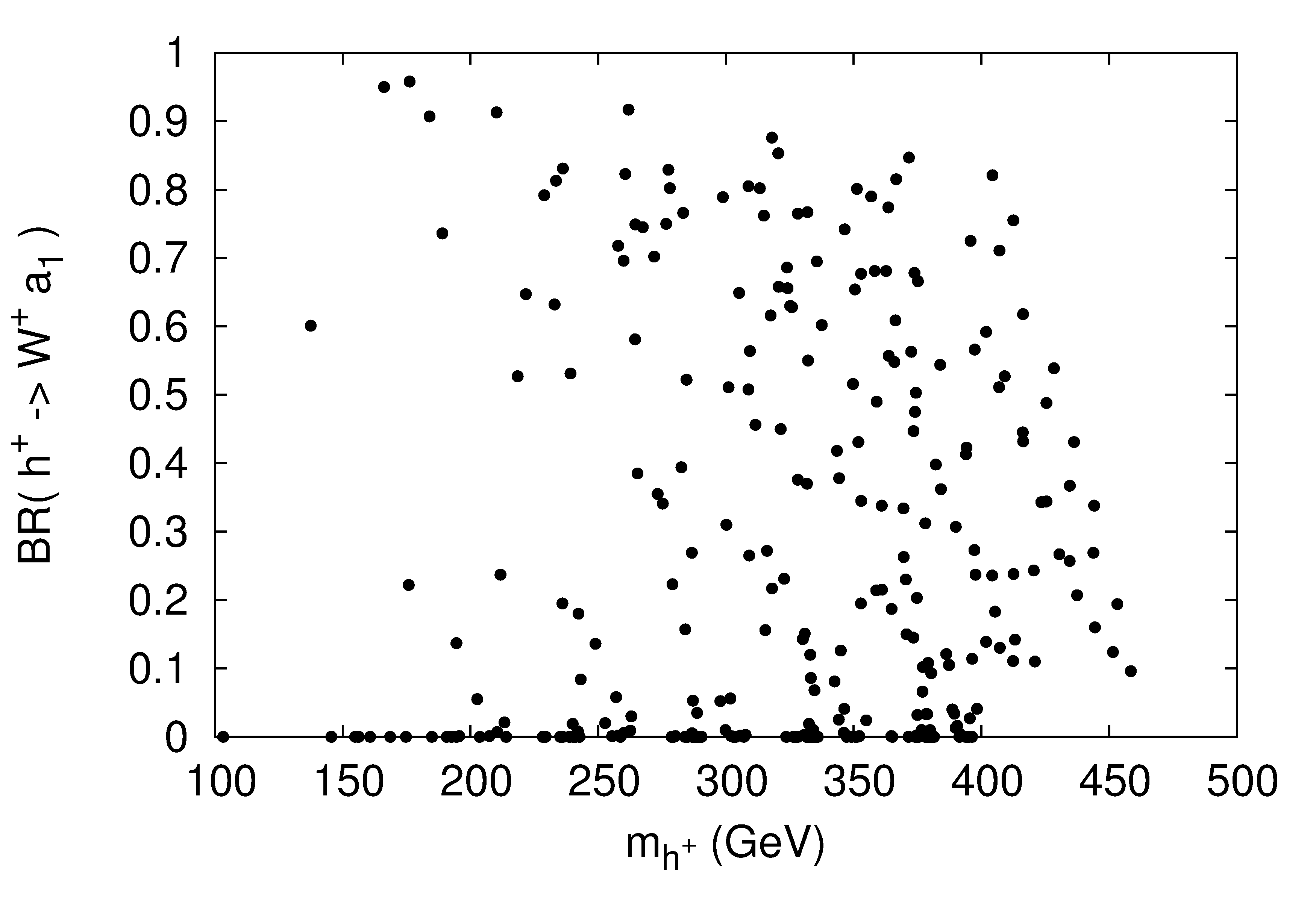
Figure 2: Top row: Charged Higgs branching ratio to $\tau\nu$ and $tb$ against $m_{h^{+}}$. Bottom row : Same with $W^{+}h_{1}$ and $W^{+}a_{1}$.

4 Benchmark points

In this section we carefully select three points which satisfy the recent bounds from LHC ATLAS ; CMS ; CMS2 and LEP LEPb to carry out the collider study. The parameters and the resulting mass spectrum for the chosen benchmark points are given in Table 1 and 2, respectively. BP1 and BP2 have larger values for $\lambda,\kappa\mathrel{\mathop{\kern 0.0pt\hbox to0.0pt{\raise 0.86108pt\hbox{$>$}\hss}}\lower 3.87495pt\hbox{\kern-1.90002pt$\sim$}}0.75$ than BP3, and the theory hits Landau pole before the GUT scale Ellwanger:2009dp . All the three benchmark points have a light, mostly singlet pseudoscalar with mass around 65-75 GeV, and is yet to be found at LHC and is allowed by the LEP data. We avoid $h_{1}\rightarrow a_{1}a_{1}$ mode by choosing $m_{a_{1}}>\frac{m_{h_{1}}}{2}$, although BR$(h_{125}\to a_{1}a_{1})\lesssim 20\%$ is still allowed with the current uncertainty hiddenHE . The charged Higgs spectrum is relatively light with the lightest one for BP3 around 182 GeV and heaviest one for BP1, around 250 GeV. For all the three benchmark points the lightest CP-even Higgs eigenstate is the discovered scalar at the LHC which satisfies the Higgs data within $2\sigma$ of the signal strengths $\mu=\frac{\sigma(pp\to h)\times\mathcal{B}(h\to XX)}{\sigma(pp\to h)_{\rm{SM}}\times\mathcal{B}(h\to XX)_{\rm{SM}}}$ in $WW^{*}$, $ZZ^{*}$ and $\gamma\gamma$ modes from ATLAS ATLAS and CMS CMS ; CMS2 . We have also taken into account the recent bounds on the third generation squarks from the LHC thridgensusy and demanded the lighter chargino to be heavier than $105$ GeV.

Parameters	BP1	BP2	BP3
$\tan\beta$	3.0	2.0	40.0
$\lambda$	0.75	0.88	0.26
$\kappa$	0.90	0.88	0.51
$A_{\kappa}$	-60.0	100.0	-100.0
$M_{A}$	270.9	245.7	280.0
$\mu$	-102.0	-200.0	190.0
$A_{t}$	75.0	100.0	1500.0

Table 1: Parameter sets chosen as the benchmark points for the collider analysis. The mass spectra are given below in Table 2.

Benchmark	BP1	BP2	BP3
Points
$m_{h_{1}}$	123.9	123.88	123.67
$m_{h_{2}}$	185.9	218.9	169.67
$m_{h_{3}}$	321.5	374.13	717.27
$m_{a_{1}}$	73.8	65.99	71.38
$m_{a_{2}}$	277.5	375.05	362.48
$m_{h^{\pm}}$	250.3	212.05	182.4
$m_{\tilde{t}_{1}}$	747.18	745.63	644.14
$m_{\tilde{t}_{2}}$	944.97	945.01	980.54
$m_{\tilde{b}_{1}}$	734.93	733.89	719.32
$m_{\tilde{b}_{2}}$	835.99	835.77	834.89

Table 2: Particle spectra for our benchmark points.

Benchmark	Branching fractions
Points	$W^{+}W^{-}$	$ZZ$	$b\bar{b}$	$\tau\bar{\tau}$
BP1	23.4%	2.8%	56.2%	5.83%
BP2	39.8%	4.89%	26.99%	2.66%
BP3	12.39%	1.52%	72.12%	8.25%

Table 3: Some major decay branching fractions of $h_{1}$ for the benchmark points.

Benchmark	Branching fractions
Points	$b\bar{b}$	$\tau\bar{\tau}$
BP1	91.1%	8.58%
BP2	91.0%	8.31%
BP3	87.95%	11.69%

Table 4: Decay branching fractions of $a_{1}$ for the benchmark points.

Table 3 presents some decay branching fractions for $h_{1}$, which is the discovered scalar around $\sim 125$ GeV. The dominant decay branching fractions are within $1\sigma$ uncertainties of both ATLAS results ATLAS and CMS CMS ; CMS2 . Table 4 presents decay branching fractions of the light pseudoscalar which dominantly decay to $b\bar{b}$ and $\tau\bar{\tau}$. From Table 5 we see that for the chosen benchmark points the light charged Higgs can decay to $a_{1}W^{\pm}$ along with the other channels ($\tau\nu$ and $tb$). BR($h^{\pm}\to a_{1}W^{\pm}$) can be as large as $\sim 66\%$ (for BP3) which shows that such a non-standard decay mode is very much possible. In the case of BP1 and BP2, $h^{\pm}\to h_{1}W^{\pm}$ mode is open but the branching fraction is rather small ($\mathrel{\mathop{\kern 0.0pt\hbox to0.0pt{\raise 0.86108pt\hbox{$<$}\hss}}\lower 3.87495pt\hbox{\kern-1.90002pt$\sim$}}1\%$). In the case of BP1, the charged Higgs decaying to lighter chargino is open via $h^{\pm}\to\tilde{\chi}^{\pm}_{1}\tilde{\chi}^{0}_{1,2,3}$ with a branching fraction of $\sim 21\%$. The charged Higgs boson decaying into supersymmetric modes could be a good probe for lighter gauginos and higgsinos at the LHC.

Benchmark	Branching fractions
Points	$h_{1}W^{\pm}$	$a_{1}W^{\pm}$	$\tau\bar{\nu}$	$t\bar{b}$
BP1	0.28%	18.9%	0.59%	59.00%
BP2	0.37%	65.6%	0.17%	33.83%
BP3	-	27.43%	60.71%	10.62%

Table 5: Some major Decay branching fractions of $h^{\pm}$ for the benchmark points.

4.1 Production processes

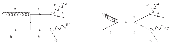
Figure 3: Feynman diagrams of $bg\to th^{\pm}$ production at the LHC.

For our case with $m_{h^{\pm}}>m_{t}$, the dominant production modes of the charged Higgs is $bg$ fusion as shown in Fig. 3. In this case we produce a single charged Higgs boson in association with a top quark. The other production modes (for e.g. pair production or $W^{\pm}$/$Z$ associated production) contribute less. The charged Higgs in NMSSM is exactly same as in MSSM or 2HDM-II. Its coupling to top and bottom quarks has two parts: one is proportional to $m_{t}\cot{\beta}$ and the other part is proportional to $m_{b}\tan{\beta}$. This feature makes the top (or bottom) mediated production modes highly $\tan\beta$ dependent as can be seen from figure 4. For BP1 such cross sections are relatively suppressed compared to BP2 (relatively lower $\tan\beta$) and BP3 (high $\tan\beta$) points respectively Datta:2001qs .

The cross sections have been calculated with the renormalization/factorization scale $Q=\sqrt{\hat{s}}$ and with CTEQ6L CTEQ as PDF. The charged Higgs can then decay to a light pseudoscalar and a $W^{\pm}$ and the top quark decays to $bW^{\pm}$ as shown in Fig. 3 thus producing in this case $1b+2W^{\pm}+a_{1}$. The light pseudoscalar will further decay into $b$ or $\tau$ pairs. This will lead to two different final states at the parton level $1b+2\tau+2\ell+\not\!\!{E_{T}}$ and $3b+2\ell+\not\!\!{E_{T}}$, if both the $W^{\pm}$ bosons decay leptonically. Table 6 shows the production cross section for the chosen benchmark points. BP3 has the largest cross section due to enhancement of the Yukawa coupling at high $\tan\beta$. Figure 4 shows the variation of $pp\to th^{\pm}$ and $pp\to tbh^{\pm}$ production cross sections at the LHC with the charged Higgs mass for a given $\tan{\beta}$. The blue dashed and green dot-dashed lines are for $\sigma(tbh^{\pm})$ at 14 TeV for $\tan\beta$ = 5 and 40, respectively. Similarly, the red dotted curve and the violet contour are for $\sigma(th^{\pm})$ at 14 TeV for $\tan\beta$ = 5 and 40, respectively.

Benchmark	Production cross sections (fb)
Points	$h^{\pm}t$	$h^{\pm}t\bar{b}$
BP1	635.00 (497.26)	376.73 (303.89)
BP2	1433.04 (1169.35)	1206.83 (979.60)
BP3	5577.89 (4572.50)	4482.60 (2421.317)

Table 6: Charged Higgs production cross sections in association with top quark and top-bottom quarks for the benchmark points for 14 (13) TeV. The renormalization/factorization scale is $Q=\sqrt{\hat{s}}$ with CTEQ6L CTEQ as PDF. K-factor is taken to be 1.55 Kidonakis:2008vd .

5 Signature and collider simulation

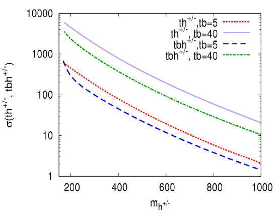
Figure 4: Cross section in fb for $pp\to th^{\pm}$ and $pp\to tbh^{\pm}$ vs mass of the charged Higgs boson. The blue, green are for $tbh^{\pm}$ and red, violet are for $th^{\pm}$ production processes at ECM=14 TeV for $\tan{\beta}=5,40$ respectively (see text). The renormalization/factorization scale is $Q=\sqrt{\hat{s}}$ with CTEQ6L CTEQ as PDF. K-factor is taken to be 1.55 Kidonakis:2008vd .

We implement the model in SARAH sarah and generate the model files for CalcHEP calchep which we use to generate the decay SLHA file. The generated events are then simulated with PYTHIA pythia via the SLHA interface slha for the decay branching and mass spectrum.

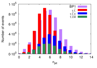
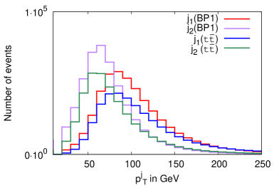
Figure 5: Jet multiplicity ($n_{j}$) distributions (left) for the signal (BP1) and dominant SM backgrounds $t\bar{t}$, $t\bar{t}Z$ and $tZW$. Jet $p_{T}$ distributions (right) of the two hardest jets (descending order in $p_{T}$) for signal (BP1) and background $t\bar{t}$.

For hadronic level simulation we have used Fastjet-3.0.3 fastjet package with the CAMBRIDGE-AACHEN algorithm ca-algo . We have set a jet size $R=0.5$ for jet formation. We have used the following isolation and selection criteria for leptons and jets:

• the calorimeter coverage is $\rm|\eta|<4.5$

• $p_{T,min}^{jet}=20$ GeV and jets are ordered in $p_{T}$

• leptons ($\rm\ell=e,\leavevmode\nobreak\ \mu$) are selected with $p_{T}\geq 20$ GeV and $\rm|\eta|\leq 2.5$

• no jet should match with a hard lepton in the event

• $\Delta R_{lj}\geq 0.4$ and $\Delta R_{ll}\geq 0.2$

• Since efficient identification of the leptons is crucial for our study, we additionally require hadronic activity within a cone of $\Delta R=0.3$ between two isolated leptons to be $\leq 0.15p^{\ell}_{T}$ GeV in the specified cone.

We consider $th^{\pm}$ and $tbh^{\pm}$ (+ h.c.) as the main production channels with charged Higgs decaying to $a_{1}W^{\pm}$. As discussed earlier, with the subsequent decays these lead to final states with $3b\,+2W^{\pm}$ or $1b+2\tau+2W^{\pm}$.

Such parton level signatures change after hadronization and in the presence of initial state and final state radiations. This changes the final state jet structure and the number of jets can increase or decrease due to these effects. In our analysis we tag a parton level tau as $\tau$-jet via its hadronic decay with at least one charged track within $\Delta R\leq 0.1$ of the candidate $\tau$-jet taujet . On the other hand, we tag a jet as $b$-jet from the secondary vertex reconstruction with single $b$-jet tagging efficiency of $0.5$ btag .

The dominant Standard Model backgrounds are $t\bar{t}+\rm{jets}$, $t\bar{t}Z$, $t\bar{t}W$. The background events (except $t\bar{t}$) are generated using CalcHEP calchep and PYTHIA pythia , then hadronized via PYTHIA. We use FastJet fastjet for jet reconstruction. $t\bar{t}$ with associated QCD jets pose serious threat to the signal. The cross section of such process is so large that even light jet faking a $\tau$-jet or a $b$-jet can reduce signal-to-background ratio. We estimate $t\bar{t}+\rm{jets}$ events using ALPGEN alpgen where we use MLM Hoche:2006ph prescription to avoid double counting of events with jets coming from hard scattering (described by matrix element method) and from soft radiation (described by parton shower models). We assume a mistagging efficiency $10^{-2}$ taumistag for a QCD jet to fake a $\tau$-jet.

In the figures the distribution of various variables are plotted at the production level without any selection cuts, in order to know their trends and differences with respect to the main SM backgrounds (due to low statistics for $t\bar{t}$-jets, we have not included that in the plots). These distributions guide us for the selection cuts leading to various final states. Figure 5 (left) describes the jet-multiplicity ($n_{j}$) distributions for the signal BP1 and the dominant SM backgrounds $t\bar{t}$, $t\bar{t}Z$ and $tZW^{\pm}$. We see that for the signal the jet-multiplicity $n_{j}$ peaks at 6. In the right panel of Fig. 5 we plot the $p^{j}_{T}$ distribution for the first and second $p_{T}$ ordered jets for the signal BP1 and for the dominant SM background $t\bar{t}$. From Fig. 5 one can see that at least the first and second jets are somewhat harder for the signal than for the background.

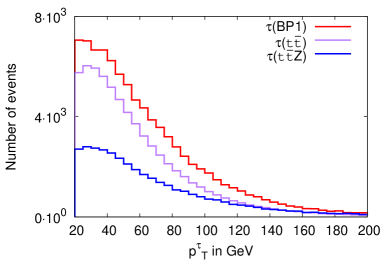
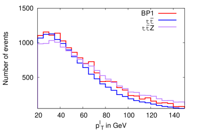
Figure 6: $\tau$-jet $p_{T}$ distribution (left) for the signal (BP1) and SM processes $t\bar{t}$, $t\bar{t}Z$. $p_{T}$ distribution of the hardest lepton (right) for signal (BP1) and SM backgrounds $t\bar{t}$, $t\bar{t}Z$.

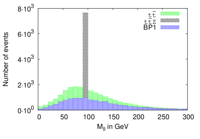
Figure 7: Lepton pair ($ee,\mu\mu$) invariant mass distribution for the signal (BP1) and dominant backgrounds $t\bar{t}$, $t\bar{t}Z$.

The left panel of Fig. 6 shows the $p_{T}$ distribution of $\tau$-jet for the signal (BP1) and for SM backgrounds $t\bar{t}$ and $t\bar{t}Z$. We see that though the $\tau$s are coming from the hidden pseudoscalar decay for the signal, they are hard enough ($p_{T}\mathrel{\mathop{\kern 0.0pt\hbox to0.0pt{\raise 0.86108pt\hbox{$>$}\hss}}\lower 3.87495pt\hbox{\kern-1.90002pt$\sim$}}$ 30 GeV) due to relatively heavier $a_{1}$ (around 70 GeV). Figure 6 (right) shows the lepton $p_{T}$ distribution for the signal (BP1) and for the SM backgrounds $t\bar{t}$, $t\bar{t}Z$. The lepton $p_{T}$s are hard enough to be detected as hard lepton as they are coming from the decays of the gauge bosons. It can be seen from Fig. 7 that the lepton pair coming from $Z$ mediated background like $t\bar{t}Z$ peaks around $m_{Z}$ in their invariant mass distribution which is not the case for the signal as they are coming from $W^{\pm}$ bosons. Thus we can use $|m_{\ell\ell}-m_{Z}|$ veto to kill the SM backgrounds coming from $Z$ boson.

5.1 $1b+2\tau+2\ell+\not\!\!{E_{T}}$

	Benchmark						Backgrounds
Final States/Cuts	BP1		BP2		BP3
	$h^{\pm}t$	$h^{\pm}bt$	$h^{\pm}t$	$h^{\pm}bt$	$h^{\pm}t$	$h^{\pm}bt$	$t\bar{t}+$jets	$tZW^{\pm}$	$t\bar{t}Z$
$n_{j}\leq 5$ $+\leavevmode\nobreak\ 2\ell$	19.89	41.94	100.56	78.37	245.96	84.94	297.69	13.1	49.66
$+|M_{\ell\ell}-M_{Z}|\geq 5$ GeV	18.90	38.90	98.23	76.41	240.62	84.94	278.95	10.07	32.54
$+|m_{\tau\tau}-M_{Z}|>10$ GeV	18.90	37.07	93.55	74.45	213.88	84.94	155.95	7.05	23.98
Significance	3.59		8.92		13.56		–

Table 7: The number of events for $n_{j}\leq 5$ (includes $1b$-jet+ $2\tau$-jet) + $2\ell$ final state at 1000 fb^-1 of luminosity at the LHC for center of mass energy (ECM) of 13 TeV.

First, we consider the pseudoscalar decay to a pair of $\tau$ jets in association with leptons coming from both the $W^{\pm}$. The final state, thus, becomes $1b+2\tau+2\ell+\not\!\!{E_{T}}$. This is relatively clean when compared with SM backgrounds. The $b$ and $\tau$ tagging reduce the dominant di-lepton backgrounds coming from the gauge boson pair in association with jets. The requirement of lower number of jets $\leq 5$ and a veto on di-lepton invariant mass around $M_{Z}$ further reduce such backgrounds. Nevertheless, we see that there are events coming from $t\bar{t}+\text{jets}$, $tZW^{\pm}$, $t\bar{t}Z$.

In Tables 7 and 8, we present the number of events coming from the signal for the three benchmark points and the SM backgrounds at an integrated luminosity of 1000 fb^-1 at 13 TeV and 14 TeV center of mass energy at the LHC, respectively. We can see that $b$-jet and $\tau$-jet invariant mass veto cuts around $M_{Z}$ help reduce the SM backgrounds. At this stage benchmark points BP2 and BP3 cross $5\sigma$ signal significance with BP3 being the highest for both cases. This shows that as early as 136 (122) fb^-1 some parameter points can be probed at the LHC with ECM of 13 (14) TeV. For BP1 and BP2 the signal significances are 3.59 (4.03) and 8.92 (8.65) respectively for 13 (14) at the LHC with 1000 fb^-1 of integrated luminosity.

We have defined $\tau$-jet via its hadronic decay with one prong charged track. A light pseudoscalar when decaying into tau pairs can give rise to two hadronic $\tau$-jets. Their invariant mass is described as $m_{\tau\tau}$ and the distribution is shown in Figure 8.

	Benchmark						Backgrounds
Final States/Cuts	BP1		BP2		BP3
	$h^{\pm}t$	$h^{\pm}bt$	$h^{\pm}t$	$h^{\pm}bt$	$h^{\pm}t$	$h^{\pm}bt$	$t\bar{t}+$jets	$tZW^{\pm}$	$t\bar{t}Z$
$n_{j}\leq 5$ $+\leavevmode\nobreak\ 2\ell$	26.67	55.76	103.18	79.65	345.72	52.42	320.23	14.54	51.88
$+|M_{\ell\ell}-M_{Z}|\geq 5$ GeV	20.32	48.97	103.18	74.82	300.06	52.42	299.06	13.57	41.51
$+|m_{\tau\tau}-M_{Z}|>10$ GeV	19.05	47.47	94.6	72.41	280.49	52.42	165.12	9.70	31.13
Significance	4.03		8.65		14.34		–

Table 8: The number of events for $n_{j}\leq 5$ (includes $1b$-jet+ $2\tau$-jet) + $2\ell$ final state at 1000 fb^-1 of luminosity at the LHC for center of mass energy (ECM) of 14 TeV.

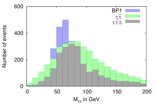
Figure 8: $\tau_{\rm jet}$ pair invariant mass distribution for the signal (BP1) and dominant backgrounds $t\bar{t}$, $t\bar{t}Z$.

5.2 $1b+2\tau+2j+1\ell+\not\!\!{E_{T}}$

	Benchmark						Backgrounds
Final States/Cuts	BP1		BP2		BP3
	$h^{\pm}t$	$h^{\pm}bt$	$h^{\pm}t$	$h^{\pm}bt$	$h^{\pm}t$	$h^{\pm}bt$	$t\bar{t}+$jets	$tZW^{\pm}$	$t\bar{t}Z$
$n_{j}\leq 6$	163.10	495.34	1014.99	854.21	2571.91	1104.25	2524.62	81.59	371.62
$+|M_{jj}-M_{W}|\leq 10$ GeV	108.40	352.51	720.32	624.98	1919.57	962.68	1783.25	64.47	309.97
$+|m_{\tau\tau}-M_{Z}|>10$ GeV	97.46	318.48	643.14	548.58	1716.39	877.73	372.78	51.37	232.90
$+m_{\tau\tau}<125.0$ GeV	92.49	288.09	605.72	505.47	1641.53	849.42	372.78	49.36	195.23
Significance	12.05		26.73		44.68		–

Table 9: The number of events for $n_{j}\leq 6$ (includes $1b$-jet+ $2\tau$-jet) + $1\ell$ final state at 1000 fb^-1 of luminosity at the LHC for center of mass energy (ECM) of 13 TeV.

In this part we consider the case when one of the $W^{\pm}$ decays hadronically. The advantage is the enhancement in signal number by a combinatoric factor of two as the other $W^{\pm}$ still decays to leptons. Both the $\tau$ and $b$ tagging keep the SM backgrounds in control. Like in the previous case, $t\bar{t}+\text{jets}$, $tZW^{\pm}$, and $t\bar{t}Z$ are the irreducible backgrounds.

Table 9 and 10 present the number of events for the benchmark points and the dominant SM backgrounds at an integrated luminosity of 1000 fb^-1 for 13 and 14 TeV center of mass energies at the LHC. For the final state we demand $n_{j}\leq 6$ (which includes $1b$-jet+ $2\tau$-jets). The rest of the jets can come from ISR, FSR or showering. Any two jets from the remaining three jets which are not tagged as $b$ or $\tau$-jets are required to have their invariant mass within 10 GeV of $M_{W}$, which reduces the combinatorial backgrounds. The requirement of ditau invariant mass outside 10 GeV of the $Z$ boson mass reduces $t\bar{t}+$jets events severely. Finally we demand the $\tau$-jet pair invariant mass to be within 125 GeV as we are looking for a light pseudoscalar which is lighter than the 125 GeV Higgs (but greater than half of it).

All the points cross $5\sigma$ signal significance for both 13 and 14 TeV energy at the LHC with the highest for BP3 of about $45\sigma$ and $51\sigma$, respectively. This shows that with a very early data, around 10 fb^-1 of integrated luminosity we can achieve $5\sigma$ significance at the LHC.

	Benchmark						Backgrounds
Final States/Cuts	BP1		BP2		BP3
	$h^{\pm}t$	$h^{\pm}bt$	$h^{\pm}t$	$h^{\pm}bt$	$h^{\pm}t$	$h^{\pm}bt$	$t\bar{t}+$jets	$tZW^{\pm}$	$t\bar{t}Z$
$n_{j}\leq 6$	200.66	602.01	1252.48	1025.81	2994.10	2149.26	2978.86	93.05	369.43
$+|M_{jj}-M_{W}|\leq 10$ GeV	153.67	437.01	879.89	731.34	2061.30	1834.74	2113.33	67.85	286.42
$+|m_{\tau\tau}-M_{Z}|>10$ GeV	135.89	394.06	773.84	661.34	1846.04	1625.05	414.82	49.43	203.40
$+m_{\tau\tau}<125.0$ GeV	115.57	366.94	742.31	605.83	1806.90	1362.95	414.82	45.56	172.26
Significance	14.45		30.29		51.40		–

Table 10: The number of events for $n_{j}\leq 6$ (includes $1b$-jet+ $2\tau$-jet) + $1\ell$ final state at 1000 fb^-1 of luminosity at the LHC for center of mass energy (ECM) of 14 TeV.

5.3 $3b+2\ell+\not\!\!{E_{T}}$

	Benchmark						Backgrounds
Final states/Cuts	BP1		BP2		BP3
	$h^{\pm}t$	$h^{\pm}bt$	$h^{\pm}t$	$h^{\pm}bt$	$h^{\pm}t$	$h^{\pm}bt$	$t\bar{t}$	$t\bar{t}Z$	$tbW$	$tZW^{\pm}$
$n_{j}\leq 5$ + $2\ell$	261.46	145.87	496.50	454.53	623.40	425.92	4165.80	39.05	8156.15	8.16
$+|m_{\ell\ell}-M_{Z}|>5$ GeV	243.96	136.14	463.29	423.58	567.09	362.03	3812.48	34.76	7422.68	7.66
$+|m_{bb}-M_{Z}|>10$ GeV	149.28	94.51	297.01	273.11	394.15	191.66	2538.92	14.04	5104.93	3.22
$+m_{bb}<125$ GeV	133.27	85.39	282.75	245.88	378.06	170.37	1774.78	12.16	3520.64	2.82
$+p_{T}^{bj_{2,3}}<100$GeV	121.33	74.45	260.06	221.0	357.95	170.37	1528.28	9.59	3168.58	1.71
Significance	2.8		6.68		7.3		–
$p_{1}:|m_{bb}-m_{a_{1}}|\leq 10\,$GeV							534.08	5.48	1202.89	1.21
	97.87		290.88		239.67		591.59	4.80	1202.89	1.11
							599.81	5.82	1408.26	1.41
Significance	2.28		6.36		5.04		–

Table 11: The number of events for $n_{j}\leq 5$ (includes $3b$-jet) + $2\ell$ final state at 100 fb^-1 of luminosity at the LHC for center of mass energy (ECM) of 13 TeV.

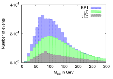
Figure 9: $b$-jet pair invariant mass distribution for the signal (BP1) and dominant backgrounds $t\bar{t}$, $t\bar{t}Z$.

Finally, we consider the case where the light pseudoscalar decays to a $b$ pair. This gives rise to a final state which constitutes of $3b+2\ell+\not\!\!{E_{T}}$ with both the $W^{\pm}$s decaying leptonically. However, at the jet level we demand $n_{j}\leq 5$ (which includes $3b$-jets).

Table 11 and 12 present the number of events for the three benchmark points and the SM backgrounds. Removal of the $\tau$-tagging from the previous cases increases the SM background contribution. This includes $t\bar{t}$, $t\bar{t}Z$, $tbW$ and $tZW^{\pm}$. To reduce these contributions we apply lepton pair invariant mass veto and $b$-jet pair invariant mass veto around the $Z$ boson mass. As in the previous case for the $\tau$-pair, we demand $b$-jet pair invariant mass to lie within 125 GeV to confirm that they can come only from the light state below 125 GeV. However, the behaviour of $tbW$ background for this final state for 13 and 14 TeV energies is not very intuitive. We can see from Table 11 and 12 that the 13 TeV numbers are greater than 14 TeV for $tbW$ process. We check via detail simulation that hadronic activity around leptons makes lepton isolation difficult for $tbW$. It is understandable that jet activity around a lepton is much enhanced as the center-of-mass energy increases from 13 TeV to 14 TeV at the LHC. This makes the number of isolated leptonic events for ECM $=14$ TeV much smaller than in case of 13 TeV. One may think that a similar observation should hold true for $t\bar{t}$ as well. We stress that the choice of our final state makes interesting impact in this case. A generic final state without any QCD radiation from $tbW$ gives $2b+2l+\not\!\!{E_{T}}$ assuming both the $W$s decay leptonically. In this case, 14 TeV numbers are greater than 13 TeV, as expected. However, in our case, the extra $b$-jet (as we demand $3b$) has to come from QCD radiation (viz, radiation from final state top or bottom) faking as $b$-jet. Hence, we are bound to take resort of extra QCD jets. Gluon emission from top does not affect much, but radiation coming from $b$ quark is more collinear for 14 TeV than for 13 TeV center-of-mass energy. Hence, jet-jet isolation criteria becomes too tight in case of 14 TeV. Thus number of events qualifying the cuts for 14 TeV become smaller than the 13 TeV numbers. On the other hand, in case of two on-shell top quarks, QCD radiation coming from one of the top quarks is enough. QCD gluon emission is more from on-shell top than from final state bottom. Hence, the same argument does not hold for $t\bar{t}$ scenario, as the $b$s (coming from top decay) and extra jet (coming as a radiation from top) are well separated to pass isolation criteria for both the center-of-mass energies.

Out of 3 $b$-jets two are coming from the light pseudoscalar in the case of the signal so we further require the $p_{T}$ of the second and third $p_{T}$ order $b$-jets to be less than 100 GeV. The signal significance at this stage are 2.8 (3.96), 6.68 (8.97) and 7.30 (12.11)$\sigma$ for BP1, BP2 and BP3, respectively, for ECM 13 (14) at the LHC.

Figure 9 shows $b$-jet pair invariant mass distribution for the BP1 and for the dominant backgrounds $t\bar{t}$ and $t\bar{t}Z$, respectively. In addition to the standard cuts as shown in Table 11 and 12, we can also use $b\bar{b}$ invariant mass cut (which peaks around the pseudoscalar mass) to achieve fairly good significance. This also gives a hint of the region where pseudoscalar mass may lie. Selection of events around 10 GeV of the $b\bar{b}$ invariant mass peak provides 2.28 (2.96), 6.36 (8.10) and 5.04 (8.19)$\sigma$ signal significances for BP1, BP2 and BP3 respectively for 13 (14) TeV at the LHC The $b\bar{b}$ peak is rather broad in Figure 9, mainly because of combinatoric factor. If we increase the selection window to $\pm 15$ ($20$) GeV around the light pseudoscalar mass peak in $b\bar{b}$ invariant mass distribution, the signal significances enhance upto 15% (23%) depending on the benchmark point.

	Benchmark						Backgrounds
Final states/Cuts	BP1		BP2		BP3
	$h^{\pm}t$	$h^{\pm}bt$	$h^{\pm}t$	$h^{\pm}bt$	$h^{\pm}t$	$h^{\pm}bt$	$t\bar{t}$	$t\bar{t}Z$	$tbW$	$tZW^{\pm}$
$n_{j}\leq 5$ + $2\ell$	313.82	180.30	564.33	546.45	804.63	670.30	5372.78	54.59	3588.78	9.89
$+|m_{\ell\ell}-M_{Z}|>5$	292.99	166.74	523.06	509.04	726.13	630.90	4920.12	47.53	3135.83	8.43
$+|m_{bb}-M_{Z}|>10$	188.470	114.60	343.93	330.43	520.06	473.10	3158.72	21.58	1986.03	4.46
$+m_{bb}<125$	167.26	104.13	328.17	299.29	466.10	394.30	2292.78	16.19	1742.13	4.36
$+p_{T}^{bj_{2,3}}<100$	150.88	92.45	304.09	270.33	441.56	354.80	1977.89	13.08	1533.07	3.78
Significance	3.96		8.97		12.11		–
$p_{1}:|m_{bb}-m_{a_{1}}|\leq 10\,$GeV							767.54	7.06	731.69	2.62
	119.46		347.50		358.52		787.22	6.23	696.85	2.42
							816.74	7.89	731.69	2.81
Significance	2.96		8.1		8.19		–

Table 12: The number of events for $n_{j}\leq 5$ (includes $3b$-jet) + $2\ell$ final state at 100 fb^-1 of luminosity at the LHC for center of mass energy (ECM) of 14 TeV.

6 Discussion and conclusions

In this paper we have considered the possibility of a hidden pseudoscalar ($\leq 100$ GeV) and a relatively light charged Higgs (just above $m_{t}$) decaying into it in the NMSSM framework. Such hidden pseudoscalar is required to have an appropriate singlet-doublet mixing in order to evade LEP bound as well as to have coupling with charged Higgs. This decay mode of the charged Higgs $h^{\pm}\rightarrow a_{1}W^{\pm}$ has not been searched by ATLAS ChATLAS or CMS ChCMS at the LHC, where finding a parameter region with a substantial branching ratio is difficult to get given the complicated parameter dependence. We have taken up a detailed collider analysis on this mode to highlight that this mode can be useful in exotic searches at the LHC.

First, we scanned a seven dimensional parameter space using the publicly available code NMSSMTools v4.7.0. We demanded the lightest CP even Higgs to have mass around 125 GeV and also to satisfy the other experimental results from the LHC. We found a suitable parameter region with a light pseudoscalar and also large branching fraction $h^{\pm}\rightarrow a_{1}W^{\pm}$. We selected three benchmark points. $\tan\beta$ is a crucial parameter in the Higgs sector. We saw that in different $\tan\beta$ regions (low, moderate and high), the charged Higgs can be just heavier than the top quark and simultaneously have a large branching ratio to $a_{1}$.

Next, we discussed the main production processes of the charged Higgs boson at the LHC. The cross section for the associated production with top quark, i.e. $pp\to th^{\pm}$ and $pp\to bth^{\pm}$, is larger than for the charged Higgs pair production. Like MSSM, NMSSM has only one physical charged Higgs boson $h^{\pm}$ and it is doublet type as singlet does not contribute to charged Higgs boson. The other production channels (e.g. charged Higgs in association with a gauge boson or SM-like Higgs) have typically smaller cross section.

The presence of a light pseudoscalar gives $b$- or $\tau$-rich final state which helps to avoid the SM backgrounds. We investigated the $1b+2\tau+2\ell+\not\!\!{p_{T}}$, $1b+2\tau+2j+1\ell+\not\!\!{p_{T}}$ and $3b+2\ell+\not\!\!{p_{T}}$ final states resulting from $W^{\pm}$ decay modes. A detailed cut-based analysis was performed in order to find a reasonably positive result in favour of our signal. We found that such scenarios can be probed with the data of as little as $\sim 10$ fb^-1 of integrated luminosity at the LHC with 13 TeV and 14 TeV center-of-mass energy.

Hidden scalars are still possible with the recent data from LHC, especially in the context of triplet-singlet extended Higgs sectors with $Z_{3}$ symmetries hiddenHE . In MSSM the heavier Higgs bosons ($h_{2},a,h^{\pm}$) are almost degenerate which rules out the possibility of $h^{\pm}\rightarrow aW^{\pm}$, where $a$ is the only massive pseudoscalar. In the case of NMSSM such hidden scalar is still allowed by LHC data and its presence prompts the decay $h^{\pm}\to a_{1}W^{\pm}$ which is not possible in the CP-conserving MSSM. In CP-violating MSSM it is possible to find a very light mostly CP-odd hidden scalar, and charged Higgs can indeed decay to $h_{1}W^{\pm}$ CPVMSSM . The triplet extended scenarios have also charged Higgs along with pseudoscalars, and can have new features, for e.g., the $Y=0$ triplet-type charged Higgs does not couple to $tb$ or $\tau\nu$ tripch . Distinguishing such charged Higgs bosons of different representations may also be possible at the LHC Bandyopadhyay:2015ifm .

Finding a charged Higgs boson will be a proof of the existence of at least another $SU(2)_{L}$ doublet or triplet scalar multiplet, and thus existence of beyond the Standard Model physics. So far LHC has searched for a charged Higgs boson decaying into $\tau\nu$ and $t\bar{b}$ which are good channels for a doublet like Higgs coupled to the fermions. To resolve the issue of the existence charged Higgs boson and its role in electroweak symmetry breaking one has to look for all possible channels.

References

- (1) ATLAS-CONF-2015-007; G. Aad et al. [ATLAS Collaboration], Phys. Rev. D 91 (2015) 1, 012006 [arXiv:1408.5191 [hep-ex]]; G. Aad et al. [ATLAS Collaboration], arXiv:1412.2641 [hep-ex]; G. Aad et al. [ATLAS Collaboration], Phys. Rev. D 90 (2014) 5, 052004 [arXiv:1406.3827 [hep-ex]].
- (2) G. Aad et al. [ATLAS and CMS Collaborations], arXiv:1503.07589 [hep-ex]; S. Chatrchyan et al. [CMS Collaboration], JHEP 1401 (2014) 096 [arXiv:1312.1129 [hep-ex]]; S. Chatrchyan et al. [CMS Collaboration], Phys. Rev. D 89 (2014) 9, 092007 [arXiv:1312.5353 [hep-ex]].
- (3) V. Khachatryan et al. [CMS Collaboration], arXiv:1412.8662 [hep-ex]; [CMS Collaboration], CMS-PAS-HIG-13-002.
- (4) E. Witten, Nucl. Phys. B 188 (1981) 513; S. Dimopoulos and H. Georgi, Nucl. Phys. B 193 (1981) 150; E. Witten, Phys. Lett. B 105 (1981) 267; R. K. Kaul and P. Majumdar, Nucl. Phys. B 199 (1982) 36; N. Sakai, Z. Phys. C 11 (1981) 153.
- (5) R. Barate et al. [LEP Working Group for Higgs boson searches and ALEPH and DELPHI and L3 and OPAL Collaborations], Phys. Lett. B 565 (2003) 61 [hep-ex/0306033]; S. Schael et al. [ALEPH and DELPHI and L3 and OPAL and LEP Working Group for Higgs Boson Searches Collaborations], Eur. Phys. J. C 47 (2006) 547 [hep-ex/0602042].
- (6) H. Baer, V. Barger and A. Mustafayev, JHEP 1205 (2012) 091 [arXiv:1202.4038 [hep-ph]]; J. Ellis and K. A. Olive, Eur. Phys. J. C 72 (2012) 2005 [arXiv:1202.3262 [hep-ph]]; P. Nath, Int. J. Mod. Phys. A 27 (2012) 1230029 [arXiv:1210.0520 [hep-ph]].
- (7) A. H. Chamseddine, R. L. Arnowitt and P. Nath, Phys. Rev. Lett. 49 (1982) 970; G. L. Kane, C. F. Kolda, L. Roszkowski and J. D. Wells, Phys. Rev. D 49 (1994) 6173 [hep-ph/9312272].
- (8) U. Ellwanger, C. Hugonie and A. M. Teixeira, Phys. Rept. 496, 1 (2010) [arXiv:0910.1785 [hep-ph]].
- (9) D. J. Miller, R. Nevzorov and P. M. Zerwas, Nucl. Phys. B 681, 3 (2004) [hep-ph/0304049]; G. G. Ross and K. Schmidt-Hoberg, Nucl. Phys. B 862 (2012) 710 [arXiv:1108.1284 [hep-ph]]; U. Ellwanger, Eur. Phys. J. C 71 (2011) 1782 [arXiv:1108.0157 [hep-ph]]; K. S. Jeong, Y. Shoji and M. Yamaguchi, JHEP 1204 (2012) 022 [arXiv:1112.1014 [hep-ph]]; N. E. Bomark, S. Moretti, S. Munir and L. Roszkowski, JHEP 1502 (2015) 044 [arXiv:1409.8393 [hep-ph]].
- (10) A. C. Bawa, C. S. Kim and A. D. Martin, Z. Phys. C 47, 75 (1990);
- (11) A. Datta, A. Djouadi, M. Guchait and Y. Mambrini, Phys. Rev. D 65, 015007 (2002) [hep-ph/0107271].
- (12) J. F. Gunion, Phys. Lett. B 322, 125 (1994) [hep-ph/9312201].
- (13) S. Andreas, O. Lebedev, S. Ramos-Sanchez and A. Ringwald, JHEP 1008 (2010) 003 [arXiv:1005.3978 [hep-ph]]; G. Cacciapaglia, A. Deandrea, G. D. La Rochelle and J. B. Flament, Phys. Rev. D 91 (2015) 1, 015012 [arXiv:1311.5132 [hep-ph]]; N. D. Christensen, T. Han, Z. Liu and S. Su, JHEP 1308 (2013) 019 [arXiv:1303.2113 [hep-ph]]; S. F. King, M. M hlleitner, R. Nevzorov and K. Walz, Phys. Rev. D 90, no. 9, 095014 (2014) [arXiv:1408.1120 [hep-ph]]; M. Guchait and J. Kumar, arXiv:1509.02452 [hep-ph].
- (14) J. Rathsman and T. Rossler, Adv. High Energy Phys. 2012, 853706 (2012) [arXiv:1206.1470 [hep-ph]].
- (15) B. Coleppa, F. Kling and S. Su, JHEP 1412, 148 (2014) [arXiv:1408.4119 [hep-ph]]; F. Kling, A. Pyarelal and S. Su, JHEP 1511, 051 (2015) [arXiv:1504.06624 [hep-ph]].
- (16) U. Ellwanger, J. F. Gunion and C. Hugonie, JHEP 0502, 066 (2005) [hep-ph/0406215]; U. Ellwanger and C. Hugonie, Comput. Phys. Commun. 175, 290 (2006) [hep-ph/0508022]; G. Belanger, F. Boudjema, C. Hugonie, A. Pukhov and A. Semenov, JCAP 0509, 001 (2005) [hep-ph/0505142].
- (17) See: http://lepsusy.web.cern.ch/lepsusy/www/inos_moriond01/charginos_pub.html
- (18) P. Bandyopadhyay, C. Coriano and A. Costantini, arXiv:1510.06309 [hep-ph]; P. Bandyopadhyay, C. Coriano and A. Costantini, JHEP 1509 (2015) 045 [arXiv:1506.03634 [hep-ph]].
- (19) G. Aad et al. [ATLAS Collaboration], arXiv:1506.08616 [hep-ex]; V. Khachatryan et al. [CMS Collaboration], JHEP 1506 (2015) 116 [arXiv:1503.08037 [hep-ex]].
- (20) J. Pumplin, D. R. Stump, J. Huston, H. L. Lai, P. Nadolsky and W. K. Tung, JHEP 0207, 012 (2002) [arXiv:hep-ph/0201195].
- (21) F. Staub, Comput. Phys. Commun. 184 (2013) pp. 1792 [Comput. Phys. Commun. 184 (2013) 1792] [arXiv:1207.0906 [hep-ph]].
- (22) A. Pukhov, “CalcHEP 3.2: MSSM, structure functions, event generation, batchs, and generation of matrix elements for other packages”, [arXiv:hep-ph/0412191].
- (23) T. Sjostrand, L. Lonnblad and S. Mrenna, [arXiv:hep-ph/0108264].
-
(24)
P. Skands et al.,
JHEP 0407, 036 (2004)
[arXiv:hep-ph/0311123];
see also http://skands.physics.monash.edu/slha/. - (25) N. Kidonakis, PoS CHARGED 2008, 003 (2008) [arXiv:0811.4757 [hep-ph]].
- (26) M. Cacciari, G. P. Salam and G. Soyez, Eur. Phys. J. C 72 (2012) 1896 [arXiv:1111.6097 [hep-ph]].
- (27) Y. L. Dokshitzer, G. D. Leder, S. Moretti and B. R. Webber, JHEP 9708, 001 (1997) [hep-ph/9707323];
- (28) G. Bagliesi, arXiv:0707.0928 [hep-ex];
- (29) I. R. Tomalin [CMS Collaboration], J. Phys. Conf. Ser. 110 (2008) 092033.
- (30) M. L. Mangano, M. Moretti, F. Piccinini, R. Pittau and A. D. Polosa, JHEP 0307, 001 (2003) doi:10.1088/1126-6708/2003/07/001 [hep-ph/0206293].
- (31) S. Hoeche, F. Krauss, N. Lavesson, L. Lonnblad, M. Mangano, A. Schalicke and S. Schumann, hep-ph/0602031.
- (32) CMS PAS TAU-11-001, See also, https://inspirehep.net/record/925248/files/TAU-11-001-pas.pdf M. Wobisch and T. Wengler, In *Hamburg 1998/1999, Monte Carlo generators for HERA physics* 270-279 [hep-ph/9907280].
- (33) G. Aad et al. [ATLAS Collaboration], JHEP 1503 (2015) 088 [arXiv:1412.6663 [hep-ex]]; G. Aad et al. [ATLAS Collaboration], arXiv:1512.03704 [hep-ex].
- (34) CMS Collaboration [CMS Collaboration], CMS-PAS-HIG-14-020; CMS Collaboration [CMS Collaboration], CMS-PAS-HIG-13-026. G. L. Bayatian et al. [CMS Collaboration], J. Phys. G 34 (2007) 995.
- (35) P. Bandyopadhyay and K. Huitu, JHEP 1311 (2013) 058 [arXiv:1106.5108 [hep-ph]]; P. Bandyopadhyay, JHEP 1108 (2011) 016 [arXiv:1008.3339 [hep-ph]]; P. Bandyopadhyay, A. Datta, A. Datta and B. Mukhopadhyaya, Phys. Rev. D 78 (2008) 015017 [arXiv:0710.3016 [hep-ph]]; D. K. Ghosh and S. Moretti, Eur. Phys. J. C 42 (2005) 341 [hep-ph/0412365]; D. K. Ghosh, R. M. Godbole and D. P. Roy, Phys. Lett. B 628 (2005) 131 [hep-ph/0412193].
- (36) P. Bandyopadhyay, K. Huitu and A. S. Keceli, JHEP 1505 (2015) 026 [arXiv:1412.7359 [hep-ph]]; P. Bandyopadhyay, S. Di Chiara, K. Huitu and A. S. Keceli, JHEP 1411 (2014) 062 [arXiv:1407.4836 [hep-ph]]; P. Bandyopadhyay, K. Huitu and A. Sabanci, JHEP 1310 (2013) 091 [arXiv:1306.4530 [hep-ph]].
- (37) P. Bandyopadhyay, C. Coriano and A. Costantini, arXiv:1512.08651 [hep-ph].