Observation of dispersive shock waves, solitons, and their interactions in viscous fluid conduits

Abstract

Dispersive shock waves and solitons are fundamental nonlinear excitations in dispersive media, but dispersive shock wave studies to date have been severely constrained. Here we report on a novel dispersive hydrodynamics testbed: the effectively frictionless dynamics of interfacial waves between two high contrast, miscible, low Reynolds’ number Stokes fluids. This scenario is realized by injecting from below a lighter, viscous fluid into a column filled with high viscosity fluid. The injected fluid forms a deformable pipe whose diameter is proportional to the injection rate, enabling precise control over the generation of symmetric interfacial waves. Buoyancy drives nonlinear interfacial self-steepening while normal stresses give rise to dispersion of interfacial waves. Extremely slow mass diffusion and mass conservation imply that the interfacial waves are effectively dissipationless. This enables high fidelity observations of large amplitude dispersive shock waves in this spatially extended system, found to agree quantitatively with a nonlinear wave averaging theory. Furthermore, several highly coherent phenomena are investigated including dispersive shock wave backflow, the refraction or absorption of solitons by dispersive shock waves, and the multi-phase merging of two dispersive shock waves. The complex, coherent, nonlinear mixing of dispersive shock waves and solitons observed here are universal features of dissipationless, dispersive hydrodynamic flows.

The behavior of a fluid-like, dispersive medium that exhibits negligible dissipation is spectacularly realized during the process of wave breaking that generates coherent nonlinear wavetrains called dispersive shock waves (DSWs). A DSW is an expanding, oscillatory train of amplitude-ordered nonlinear waves composed of a large amplitude solitonic wave adjacent to a monotonically decreasing wave envelope that terminates with a packet of small amplitude dispersive waves. Thus, DSWs coherently encapsulate a range of fundamental, universal features of nonlinear wave systems. More broadly, DSWs occur in dispersive hydrodynamic media that exhibit three unifying features: i) nonlinear self-steepening, ii) wave dispersion, iii) negligible dissipation (c.f. the comprehensive DSW review article El (2016)).

Dispersive shock waves and solitons are ubiquitous excitations in dispersive hydrodynamics, having been observed in many environments such as quantum shocks in quantum systems (ultra-cold atoms Dutton et al. (2001); Hoefer et al. (2006), semiconductor cavities Amo et al. (2011), electron beams Mo et al. (2013)), optical shocks in nonlinear photonics Rothenberg and Grischkowsky (1989), undular bores in geophysical fluids Hammack and Segur (1978); Farmer and Armi (1999), and collisionless shocks in rarefied plasma Taylor et al. (1970). However, all DSW studies to date have been severely constrained by expensive laboratory setups Dutton et al. (2001); Hoefer et al. (2006); Mo et al. (2013); Hammack and Segur (1978) or challenging field studies Farmer and Armi (1999), difficulties in capturing dynamical information Rothenberg and Grischkowsky (1989); Dutton et al. (2001); Hoefer et al. (2006), complex physical modeling Farmer and Armi (1999), or a loss of coherence due to multi-dimensional instabilities Dutton et al. (2001); Amo et al. (2011) or dissipation Taylor et al. (1970); Mo et al. (2013). Here we report on a novel dispersive hydrodynamics testbed that circumvents all of these difficulties: the effective superflow of interfacial waves between two high viscosity contrast, low Reynolds number Stokes fluids. The viscous fluid conduit system was well-studied in the 1980s as a simplified model of magma transport through the Earth’s partially molten upper mantle Scott and Stevenson (1984); Scott et al. (1986); Whitehead and Helfrich (1988) (see also the background material in _se ). This system enables high fidelity studies of large amplitude DSWs, which are found to agree quantitatively with nonlinear wave averaging or Whitham theory Whitham (1974); Gurevich and Pitaevskii (1974); Lowman and Hoefer (2013a). We then report the first experimental observations of highly coherent phenomena including DSW backflow, the refraction or absorption of solitons interacting with DSWs, and multi-phase DSW-DSW merger. In addition to its fundamental interest, the nonlinear mixing of mesoscopic scale solitons and macroscopic scale DSWs could play a major role in the initiation of decoherence and a one-dimensional, integrable turbulent state El and Kamchatnov (2005) that has recently been observed in optical fibers Randoux et al. (2014) and surface ocean waves Costa et al. (2014).

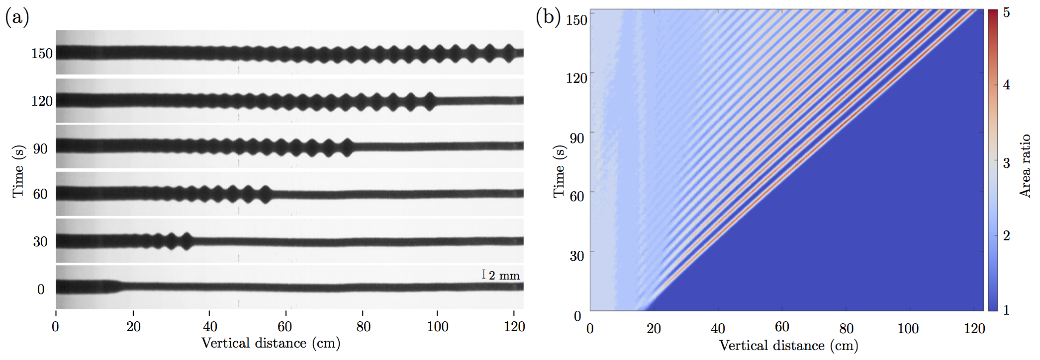
Figure 1: Interfacial wave breaking of two Stokes fluids causing the spontaneous emergence of coherent oscillations, a DSW. The leading, downstream edge is approximately a large amplitude soliton whose phase speed is tied to the upstream conduit area. The trailing, upstream edge is a small amplitude wave packet moving at the group velocity whose wavenumber is tied to the downstream conduit area. (a) 90^∘ clockwise rotated, time-lapse digital images (aspect ratio 10:1). (b) Space-time contour plot of the conduit cross-sectional area from (a). Nominal experimental parameters: $\Delta\rho=0.0928$ g/cm³, $\mu_{\rm i}=91.7$ cP, $\epsilon=0.030$, downstream flow rate $Q_{0}=0.50$ mL/min, and $a_{-}=2.5$.

In our experiment, the steady injection of an intrusive viscous fluid (dyed, diluted corn syrup) into an exterior, miscible, much more viscous fluid (pure corn syrup) leads to the formation of a stable fluid filled pipe or conduit Whitehead and Luther (1975). Due to high viscosity contrast, there is minimal drag at the conduit interface so the flow is well approximated by the Poiseulle or pipe flow relation $D\propto Q^{1/4}$ where $Q$ is the injection rate and $D$ is the conduit diameter. By modulating the injection rate, interfacial wave dynamics ensue. Dilation of the conduit gives rise to buoyancy induced nonlinear self-steepening regularized by normal interfacial stresses that manifest as interfacial wave dispersion Olson and Christensen (1986); Lowman and Hoefer (2013b). Negligible mass diffusion implies a sharp conduit interface and conservation of injected fluid. By identifying the azimuthally symmetric conduit interface as our one-dimensional dispersive hydrodynamic medium, we arrive at the counterintuitive behavior that viscous dominated, Stokes fluid dynamics exhibit dissipationless or frictionless interfacial wave dynamics. This will be made mathematically precise below.

By gradually increasing the injection rate, we are able to initiate the spontaneous emergence of interfacial wave oscillations on an otherwise smooth, slowly varying conduit. See _se for additional experimental details. Figure 1(a) displays a typical time-lapse of our experiment. At time $0$ s, the conduit exhibits a relatively sharp transition between narrower and wider regions. Due to buoyancy, the interface of the wider region moves faster than the narrower region. Rather than experience folding over on itself, the interface begins to oscillate due to dispersive effects as shown in Fig. 1(a) at 30 s. As later times in Fig. 1(a) attest, the oscillatory region expands while the oscillation amplitudes maintain a regular, rank ordering from large to small. By extracting the spatial variation of the normalized conduit cross-sectional area $a$ from a one frame per second image sequence, we display in Fig. 1(b) the full spatio-temporal interfacial dynamics as a contour plot. This plot reveals two characteristic fronts associated with the oscillatory dynamics: a large amplitude leading edge and a small amplitude, oscillatory envelope trailing edge.

We can interpret these dynamics as a DSW resulting from the physical realization of the Gurevich-Pitaevskii (GP) problem Gurevich and Pitaevskii (1974), a standard textbook problem for the study of DSWs El (2016) that has been inaccessible in other dispersive hydrodynamic systems. Here, the GP problem is the dispersive hydrodynamics of an initial jump in conduit area. Although we have only boundary control of the conduit width, our carefully prescribed injection protocol _se enables delayed breaking far from the injection site. This allows for the isolated creation and long-time propagation of a “pure” DSW connecting two uniform, distinct conduit areas. Related excitations in the conduit system were previously interpreted as periodic wave trains modeling mantle magma transport Scott et al. (1986). As we now demonstrate, the interfacial dynamics observed here exhibit a soliton-like leading edge propagating with a well-defined nonlinear phase velocity, an interior described by a modulated nonlinear traveling wave, and a harmonic wave trailing edge moving with the linear group velocity. The two distinct speeds of wave propagation in one coherent structure are a striking realization of the double characteristic splitting from linear wave theory Whitham (1974).

The long wavelength approximation of the interfacial fluid dynamics is the conduit equation Scott et al. (1986); Lowman and Hoefer (2013b)

$$a_{t}+\left(a^{2}\right)_{z}-\left(a^{2}\left(a^{-1}a_{t}\right)_{z}\right)_{z}=0\ .$$ (1)

Here, $a(z,t)$ is the nondimensional cross-sectional area of the conduit as a function of the scaled vertical coordinate $z$ and time $t$ (subscripts denote partial derivatives). Both the interface of the experimental conduit system and equation (1) exhibit the essential features of frictionless, dispersive hydrodynamics: nonlinear self-steepening (second term) due to buoyant advection of the intrusive fluid, dispersion (third term) from normal stresses, and no dissipation due to the combination of intrusive fluid mass conservation and negligible mass diffusion _se . The analogy to frictionless flow corresponds to the interfacial dynamics, not the momentum diffusion dominated flow of the bulk. The conduit equation (1) is nondimensionalized according to cross-sectional area, vertical distance, and time in units of $A_{0}=\pi R_{0}^{2}$, $L_{0}=R_{0}/\sqrt{8\epsilon}$, and $T_{0}=\mu_{\rm i}/L_{0}g\Delta\rho\epsilon$, respectively, where $R_{0}$ is the downstream conduit radius, $\epsilon=\mu_{\rm i}/\mu_{\rm e}$ is the viscosity ratio of the intrusive to exterior liquids, $\Delta\rho=\rho_{\rm e}-\rho_{\rm i}$ is the density difference, and $g$ is gravity acceleration. Initially proposed as a simplified model for the vertical ascent of magma along narrow, viscously deformable dikes and principally used to study solitons Scott et al. (1986); Olson and Christensen (1986); Helfrich and Whitehead (1990), the conduit equation (1) has since been derived systematically from the full set of coupled Navier-Stokes fluid equations using a perturbative procedure with the viscosity ratio as the small parameter Lowman and Hoefer (2013b). The conduit equation (1) was theoretically shown to be valid for long times and large amplitudes under modest physical assumptions on the basin geometry, background velocities, fluid compositions, weak mass to momentum diffusion, and characteristic aspect ratio. The efficacy of this model has been experimentally verified in the case of solitons Olson and Christensen (1986); Helfrich and Whitehead (1990).

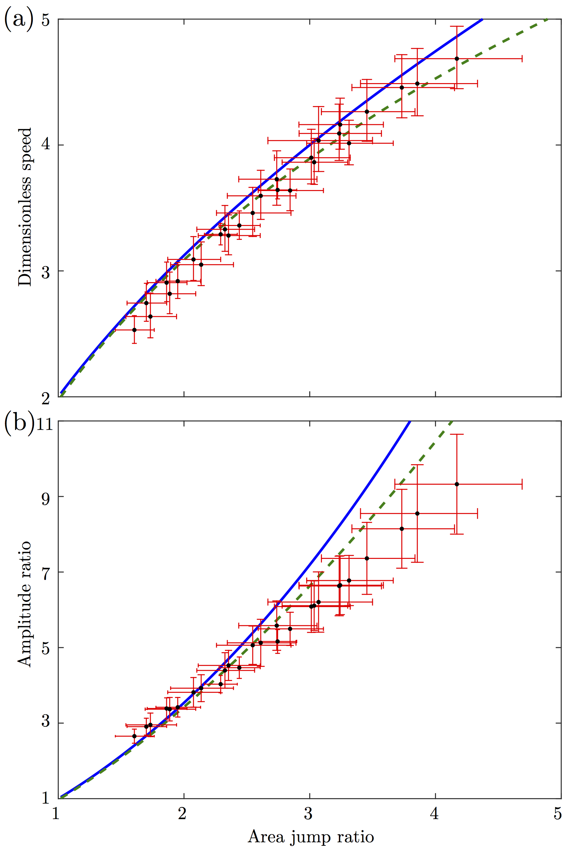
Figure 2: Comparison of observed and predicted leading edge DSW amplitude and speed. Observations (circles), Whitham modulation theory (solid), and numerical simulation of the conduit equation (dashed) for (a) DSW leading edge speeds $s_{+}$ and (b) DSW leading amplitude $a_{+}$ versus downstream area ratio $a_{-}$. Nominal experimental parameters: $\Delta\rho=0.1305$ g/cm³, $\mu_{\rm i}=80.4$ cP (measured), $\mu_{\rm i}=104$ cP (fitted), $\epsilon=0.0024$. See _se for fitting procedure.

The study of DSWs involves a nonlinear wave modulation theory, commonly referred to as Whitham theory Whitham (1974), which treats a DSW as an adiabatically modulated periodic wave Gurevich and Pitaevskii (1974); El (2016). Using Whitham theory and eq. (1), key conduit DSW physical features such as leading soliton amplitude and leading/trailing speeds have been determined Lowman and Hoefer (2013a). For the jump in downstream to upstream area ratio $a_{-}$, Whitham theory applied to the conduit equation (1) predicts relatively simple expressions for the DSW leading $s_{+}$ and trailing $s_{-}$ edge speeds

$$s_{+}=\sqrt{1+8a_{-}}-1,\quad s_{-}=3+3a_{-}-3\sqrt{a_{-}(8+a_{-})},$$ (2)

in units of the characteristic speed $U_{0}=L_{0}/T_{0}$. The leading edge approximately corresponds to an isolated soliton where the modulated periodic wave exhibits a zero wavenumber. Given the speed $s_{+}$, the soliton amplitude $a_{+}$ is implicitly determined from the soliton dispersion relation $s_{+}=[a_{+}^{2}(2\ln a_{+}-1)+1]/(a_{+}-1)^{2}$ Olson and Christensen (1986). At the trailing edge, the modulated wave limits to zero amplitude, corresponding to harmonic waves propagating with the group velocity $s_{-}=\omega^{\prime}(k_{-})$, where $\omega(k)=2a_{-}k/(1+a_{-}k^{2})$ is the linear dispersion relation of eq. (1) on a background conduit area $a_{-}$ and $k_{-}^{2}=(a_{-}-4+\sqrt{a_{-}(8+a_{-})})/(4a_{-})$ is the distinguished wavenumber determined from modulation theory Lowman and Hoefer (2013a) (see also El (2016)).

In Fig. 2, we compare the leading edge amplitude and speed predictions with experiment, demonstrating quantitative agreement for a range of jump values $a_{-}$. The analytical theory (Whitham theory) is known to break down at large amplitudes Lowman and Hoefer (2013a) so we also include direct determination of the speed and amplitude from numerical simulation of eq. (1), demonstrating even better agreement. In order to obtain the reported dimensionless speeds of Fig. 2(a), we divide the measured speeds by $U_{0}$ with $\mu_{\rm i}$ determined by fitting the downstream conduit area to a Poiseulle flow relation. This enables us to self-consistently account for the shear-thinning properties of corn syrup. All the remaining fluid parameters take their nominal, measured values. The deviation between experiment and theory at large jump values is consistent with previous measurements of solitons, where the soliton dispersion relation was found to underpredict observed speeds at large amplitudes Olson and Christensen (1986) (see also _se ).

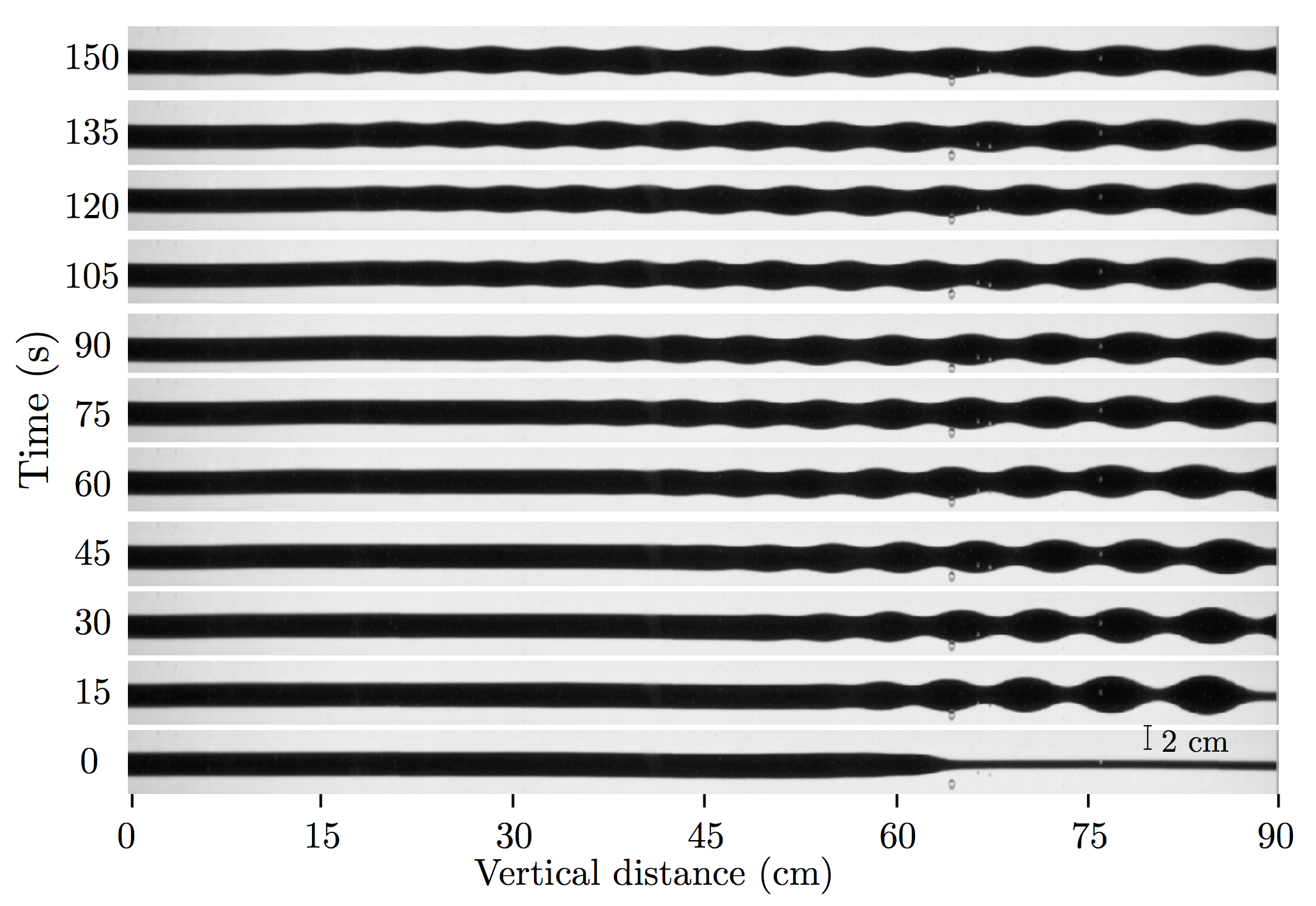
Figure 3: Time-lapse images (aspect ratio 1:1) of large amplitude wave breaking leading to upstream propagation of the DSW trailing edge envelope: DSW backflow. Nominal experimental parameters: $\Delta\rho=0.0983$ g/cm³, $\mu_{\rm i}=93.5$ cP, $\epsilon=0.029$, $a_{-}=4$, and $Q_{0}=0.50$ mL/min.

In addition to single DSWs, our experimental setup allows us to investigate exotic, coherent effects predicted by eq. (1) for the first time. For example, backflow is a feature of dispersive hydrodynamic systems whereby a portion of the DSW envelope propagates upstream. This feature occurs here when the group velocity of the trailing edge wave packet is negative. From the expression for $s_{-}$ in (2), we predict the onset of backflow when $a_{-}$ exceeds $8/3$. In Fig. 3, we utilize our injection protocol to report the observation of this phenomenon in the viscous conduit setting (see _se for video). Waves with strictly positive phase velocity are continually generated at the trailing edge but the envelope group velocity is negative. We estimate the crossover to backflow for the experiments reported in Fig. 2 at $a_{-}\approx 3$, consistent with a slightly larger crossover than theory (8/3) due to sub-imaging-resolution of small amplitude waves.

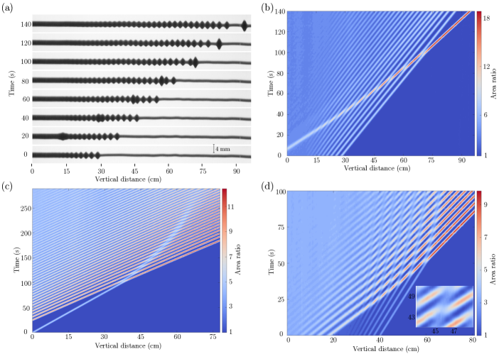
Figure 4: Interactions of solitons and DSWs. Time-lapse images with aspect ratio 10:1 (a) and space-time contour (b) of DSW-soliton interaction revealing soliton refraction by a DSW with $a_{-}=3$. (c) Space-time contour of the absorption of a soliton by a DSW with $a_{-}=3.5$. (d) DSW-DSW interaction and merger causing multiphase mixing (inset) and the refraction of the trailing DSW by the leading DSW with $a_{1}=2.5$, $a_{2}=5$. Nominal experimental parameters: $\Delta\rho=0.0971$ g/cm³, $\mu_{\rm i}=99.1$ cP, $\epsilon=0.029$, $Q_{0}=0.2$ mL/min.

The ease with which DSWs and solitons can be created in this viscous liquid conduit system enables the investigation of novel coherent, nonlinear wave interactions. In Fig. 4, we report soliton-DSW and DSW-DSW interactions from our conduit experiment (see _se for videos). As in previous experiments Olson and Christensen (1986); Helfrich and Whitehead (1990), an isolated conduit soliton is created by the pulsed injection of fluid on top of the steady injection that maintains the background conduit. Figures 4(a,b) depict the generation of a DSW followed by a soliton. Because solitons propagate with a nonlinear phase velocity larger than the linear wave phase and group velocities Olson and Christensen (1986), the soliton eventually overtakes the DSW trailing edge. The soliton-DSW interaction results in a sequence of phase shifts between the soliton and the crests of the modulated wavetrain. The soliton emerges from the interaction with a significantly increased amplitude and decreased speed due to the smaller downstream conduit upon which it is propagating. The initial and final slopes of soliton propagation in Fig. 4(b) demonstrate that the soliton has been refracted by the DSW. Meanwhile, the DSW experiences a subtle phase shift and is otherwise unchanged.

The opposite problem of a soliton being overtaken by a DSW is displayed in Fig. 4(c). After multiple phase shifts during interaction, the soliton is slowed down and effectively absorbed within the interior of the DSW, while the DSW is apparently unchanged except for a phase shift in its leading portion. Such behavior is consistent with the interpretation of a DSW as a modulated wavetrain with small amplitude trailing waves that will always move slower than a finite amplitude soliton.

Figure 4(d) reveals the interaction of two DSWs. The interaction region results in a series of phase shifts due to soliton-soliton interactions that form a quasiperiodic or two-phase wavetrain as shown in the inset. This nonlinear mixing eventually subsides, leaving a single DSW representing the merger of the original two. The trailing DSW has effectively been refracted by the leading DSW.

We can interpret the soliton and DSW refraction as follows. First, consider the overtaking interaction of two DSWs. Denote the midstream and upstream conduit areas $a_{1}<a_{2}$ relative to the downstream area $a_{0}=1$. Equation (2) implies the leading edge speeds of the first and second DSWs are $s_{1}=\sqrt{1+8a_{1}}-1$, $s_{2}=a_{1}(\sqrt{9+8(a_{2}-1)/a_{1}}-1)$. Motivated by previous DSW interaction studies Ablowitz et al. (2009), we assume merger of the two DSWs and thus obtain the leading edge speed of the merged DSW $s_{m}=4\sqrt{\frac{1}{2}(a_{1}+a_{2})-1}-1$ connecting conduit areas $a_{0}$ to $a_{2}$. One can verify the interleaving property $s_{1}<s_{m}<s_{2}$, demonstrating the refraction (slowing down) of the second DSW. If we treat the isolated soliton as the leading edge of a DSW, then we obtain the same result for soliton-DSW refraction.

Viscous liquid conduits are a model system for the coherent dynamics of one-dimensional superfluid-like media with microscopic-scale fluid dynamics Whitehead and Helfrich (1988), mesoscopic-scale solitons Helfrich and Whitehead (1990) and macroscopic-scale DSWs as fundamental nonlinear excitations. Interaction of DSWs and solitons suggest that soliton refraction, absorption, multi-phase dynamics, and DSW merging are general, universal features of dispersive hydrodynamics. The viscous liquid conduit system is a new environment in which to investigate complex, coherent dispersive hydrodynamics that have been inaccessible in other superfluid-like media.

In this supplemental material, background information and additional experimental details are provided.

I Background on viscous fluid conduits

Principally driven by the modeling of geological and geophysical processes, Whitehead and Luther in 1975 showed that the low Reynolds number, buoyant dynamics of two fluids with differing densities and viscosities could lead to the formation of stable fluid filled pipes or conduits of upwelling fluid Whitehead and Luther (1975). In 1984, McKenzie derived a system of equations describing the dynamics of melt (magma) within a deformable matrix (rock) in the upper Earth’s mantle McKenzie (1984). These equations treat the magma dynamics as the flow of a low Reynolds number, incompressible fluid through a more viscous, permeable matrix that is modeled as a compressible fluid due to compaction and distension. There are two model parameters $(n,m)$ resulting from constitutive power laws that relate the porosity to the matrix permeability and viscosity, respectively. Soon after, it was realized that the asymptotically reduced, one-dimensional McKenzie equations, or magma equation, exhibits solitary wave solutions Scott and Stevenson (1984). A connection between the laboratory fluid systems explored by Whitehead and Luther and the magma equation was realized in Olson and Christensen (1986); Scott et al. (1986) where the conduit equation studied in the present work (eq. 1 in the primary manuscript) was derived from physical arguments, the soliton amplitude-speed relation was verified experimentally, and the approximately elastic solitonic interaction property was observed. The conduit equation corresponds exactly to the magma equation when $(n,m)=(2,1)$. Since that time, there have been a number of experimental and theoretical works on viscous fluid conduits, principally focused upon the dynamics of solitons (see, e.g., whitehead (1990); Simpson and Weinstein (2008) and references therein). It is now known that the one- and two-dimensional solitary wave solutions to McKenzie’s equations are unstable to transverse perturbations, leading to the formation of fully three-dimensional solitary waves Wiggins and Spiegelman (1995).

In this work, rather than emphasize the connection to McKenzie’s equations and magma dynamics, we consider the dynamics of viscous fluid conduits as a model dispersive hydrodynamic system where hydrodynamic nonlinearity is balanced by dispersive effects. Such systems are plentiful in the natural world, as commented upon in the introduction of the accompanying manuscript. In addition to solitons, dispersive shock waves (DSWs) are fundamental nonlinear excitations in dispersive hydrodynamic media (see the review El (2016)). The first numerical studies of DSWs in the McKenzie equations was undertaken by Spiegelman Spiegelman (1993). Whitham modulation theory was later used to describe DSWs in the small Elperin et al (1994) and large Marchant and Smyth (2005); Lowman et al. (2014) amplitude regimes of the magma and, in particular, the conduit equation. The present work represents the first experimental study of conduit DSWs.

II Poiseuille flow relation

The conduit experimental data are obtained by injecting through a 0.22 cm inner diameter nozzle an approximately 7:2:1 mixture of corn syrup (Karo brand light), water, and black food coloring (Regal brand) into the bottom of a 2 m tall acrylic, 25.8 cm² square column filled with corn syrup (3:2 mixture of Golden Barrel brand 42 dextrose equivalent and Karo brand light for data of Figure 2, pure Karo brand light for Figures 1, 3, 4). The fluid temperature near the top of the fluid column was measured to be $22.2\pm 0.7$ deg C across all experimental trials. A computer controlled piston pump (Global FIA milliGat LF pump with MicroLynx controller) was used to inject fluid through a room temperature water bath followed by the nozzle. See Fig. S1 for an experimental schematic. When the injected fluid reaches the top of the fluid column, it pools on top of the external fluid and very slowly begins to diffuse downward. We periodically removed the pooling fluid with a syringe. Steady injection results in a vertically uniform liquid filled pipe or conduit conforming to Poiseuille flow Whitehead and Luther (1975); Scott et al. (1986). We allowed the conduit to stabilize (straighten) by steady injection over a period of 36 hours for the data in Fig. 2 and 15 hours for the other data.

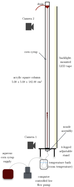
Figure S1: Schematic of the conduit experimental apparatus.

The quantitative data in Fig. 2 exhibits typical conduit diameters of one to four millimetres and Reynolds numbers in the range Re $=\rho_{\rm i}U_{0}L_{0}/\mu_{\rm i}\in(0.06,2.6)$, where $\rho_{\rm i}$ is the intrusive fluid density. We can set the conduit diameter $D$ via the volumetric flow rate $Q$ according to a Hagan-Poiseuille relation Whitehead and Luther (1975) $D=\alpha Q^{1/4}=(2^{7}\mu_{\rm i}Q)^{1/4}/(\pi g\Delta\rho)^{1/4}$. Digital images of the conduit are processed to extract the conduit diameter. The conduit edges are determined from local extrema of the differentiated grayscale intensity image using centred differences in the direction normal to the conduit interface. We confirm the Poiseuille flow relation $D=\alpha Q^{1/4}$ for the trials of Fig. 2 approximately 6 cm above the fluid injection site with no fitting parameters (Fig. S2). In Fig. S3, we show the fit of the Poiseuille flow relation to the same conduit, imaged approximately 120 cm above the injection site. The difference between the externally measured viscosity $\mu_{\rm i}=80.4$ cP and the value $\mu_{\rm i}=104$ cP from a fit to the Poiseuille flow relation can be explained by the non-Newtonian, thixotropic (shear thinning) properties of corn syrup. At the injection site, the diluted corn syrup experiences heightened shearing, similar to our rotational viscometer measurements (Brookfield DV-I prime viscometer). Further up the fluid column, there is less shearing so the fluid increases in viscosity and leads to a dilation of the conduit. The conduit consistently has a measured diameter in the upper fluid column that is 7% larger than its value near the injection site as shown in Fig. S4. The results in Fig. 2 of the main text use the measured value of $\Delta\rho$ and the fitted value $\mu_{\rm i}=104$ cP.

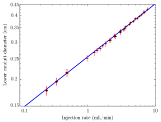
Figure S2: Demonstration of Poiseuille flow in a steady viscous fluid conduit. Log-log plot of measured conduit diameter $D$ near injection site versus volumetric flow rate $Q$ (dots) and the relation $D=\alpha Q^{1/4}$ with the measured value $\alpha=0.2557$ (cm$\cdot$min)^1/4 (solid) corresponding to $\mu_{\rm i}=80.4$ cP, $\Delta\rho=0.1305$ g/cm³. A least squares fit gives $\alpha=0.2548$ (cm$\cdot$min)^1/4, which translates to the fitted viscosity $\mu_{\rm i}=79.0$ cP, within the 2% error tolerance of our rotational viscometer.

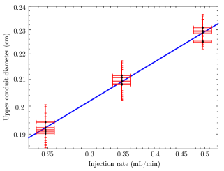
Figure S3: Poiseuille flow fit approximately 120 cm up the fluid column. Downstream conduit diameters $D$ extracted from digital images (dots) and a least squares fit to the Poiseuille flow relation $D=\alpha Q^{1/4}$ with $\alpha=0.2688$ (cm$\cdot$min)^1/4 (solid). The fit corresponds to the interior viscosity $\mu_{\rm i}=104$ cP, an increase from its measured value $\mu_{\rm i}=80.4$ cP. This can be explained by the shear thinning properties of corn syrup as described in Methods.

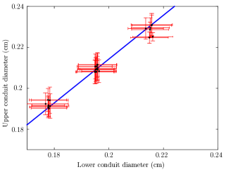
Figure S4: Comparison of conduit diameter at different locations along the fluid column. Measurements (dots) and the linear fit $D_{\rm top}=mD_{\rm bottom}$ (solid) with $m=1.07$ corresponding to a 7% increase in the conduit diameter. The lower (upper) diameter was measured approximately 6 cm (120 cm) above the injection site.

III DSW and soliton injection protocol.

By adiabatically changing $Q$, we introduce perturbations to the conduit that subsequently propagate along the interface, allowing for the generation of conduit solitons Olson and Christensen (1986); Whitehead and Helfrich (1988); Helfrich and Whitehead (1990); Lowman et al. (2014) and DSWs. The injection rate profile for solitons is generated by computing a conduit solitary wave solution $a_{\rm soliton}(z-ct-z_{0})$ with speed $c$ and initial center $z_{0}$ to eq. (1). This profile is converted to the dimensional diameter $D_{\rm soliton}=2\sqrt{a_{\rm soliton}A_{0}/\pi}$ and then the volumetric flow rate profile $Q_{\rm soliton}=(D_{\rm soliton}/\alpha)^{4}$, evaluated at the injection site.

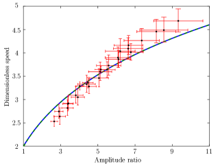
Figure S5: DSW leading edge speed versus amplitude. The observed values (dots) and the theoretical soliton dispersion relation (solid) corresponding to Fig. 2(a,b) in the main text. The deviation at large amplitudes is consistent with previous studies of isolated solitons Olson and Christensen (1986).

The volumetric flow rate profile $Q_{\rm DSW}$ that we use to create DSWs is determined as follows. We initialize the dispersionless conduit equation $a_{t}+\left(a^{2}\right)_{z}=0$ with a step in conduit area from $a_{-}$ to 1, left to right, at a desired distance from the nozzle $z=z_{b}$. Evolving this initial value problem backward in time results in a non-centered rarefaction wave that can be related to the volumetric flow rate profile via

$$Q_{\rm DSW}(\tau)=Q_{0}\begin{cases}1&t\leq 0\\ (1-2\tau U_{0}/Z_{b})^{-2}&0<\tau U_{0}/Z_{b}<(a_{-}-1)/2a_{-}\\ a_{-}^{2}&\mathrm{else}\end{cases},$$

where $Q_{0}$ is the downstream flow rate, $\tau$ is the dimensional time, and $Z_{b}=L_{0}z_{b}$ is the dimensional breaking distance from the injection site. We find that this provides adequate control over the breaking location.

Each DSW trial in Fig. 2 was initiated after a sufficient waiting period, typically 5 minutes, to allow the previous trial’s conduit diameter to stabilize to the expected steady value. The downstream flow rates utilized for the data in Fig. 2 were nominally $Q_{0}\in\{0.25,0.35,0.5\}$ mL/min. Three digital SLR cameras were utilized, two Canon EOS 70D camers outfitted with Tamron macro lenses positioned just above the injection site (camera one) and at approximately 120 cm above the injection site (camera two). The third camera (Canon EOS Rebel T5i), outfitted with a zoom lens, was used to image the entire vertical length of 120 cm from the injection site. The fluid column was backlit with strip LED lights behind LEE LE251R white diffusion filter paper. Each DSW trial was initiated with an image of the conduit at the injection site followed by the injection protocol $Q_{\rm DSW}$. The third camera was then set to image the full column every second throughout the trial. Just after the injection protocol reached the maximum rate $a_{-}Q_{0}$, an image of the conduit from camera 1 was taken. Just prior to the arrival of the DSW leading edge within the viewing area of camera two, an image of the downstream conduit was taken, followed by a dozen or more images taken in rapid succession of the DSW leading edge.

IV Determination of DSW speed and amplitude.

The leading edge of the DSW amplitude, normalised to the downstream area, is determined from the digital images of camera 2 without appealing to any fluid parameters. We compute the conduit edges as for the steady case, using extrema of the differentiated image intensity normal to the conduit interface. Some image and edge smoothing is performed to remove pixel noise. The number of pixels across the diameter of the leading edge DSW peak is calculated and normalized by the diameter of the downstream conduit. Squaring this quantity gives the leading edge DSW amplitude shown in Fig. 2. We calculated the leading edge DSW speed from the images of camera three toward the end of the trial. We nondimensionalise the speed by the characteristic speed $U_{0}=L_{0}/T_{0}=gA_{0}\Delta\rho/(8\pi\mu_{\rm i})$, where we use the measured values of the downstream flow area $A_{0}$ from camera two and $\Delta\rho$. The fitted value for $\mu_{\rm i}$ is used, as described in the earlier section on Poiseuille flow.

V Mass diffusion.

The injected and external fluids are miscible so there is unavoidable mass diffusion across an interface between the two. Using a procedure similar to that described in Ray et al. (2007), we estimate the diffusion constant $\tilde{D}$ between a 7:3 corn syrup, water mixture and pure corn syrup (Karo brand light) to be approximately $1.2\times 10^{-6}$ cm²/s. Combining this with typical flow parameters, we estimate the Péclet and Schmidt numbers for the trials of Fig. 2 to lie in the range Pe = $L_{0}U_{0}/\tilde{D}\in(2.1\times 10^{4},7.9\times 10^{5})$ and Sc = Pe/Re $\approx 5.2\times 10^{5}$. The advective time scale for Fig. 2 trials is in the range $T_{0}\in(1.6,5.6)$ s. We therefore estimate that mass diffusion begins to play a role after approximately 9 hours, whereas the time scale of an experimental trial is less than 10 minutes.

References

- Whitehead and Luther (1975) J. A. Whitehead and D. S. Luther, J. Geophys. Res. 80, 705 (1975).
- McKenzie (1984) D. McKenzie, J. Petrology 25, 713 (1984).
- Scott and Stevenson (1984) D. R. Scott, and D. J. Stevenson, Geophys. Res. Lett. 11, 1161 (1984).
- Scott et al. (1986) D. R. Scott, D. J. Stevenson, and J. A. Whitehead, Nature 319, 759 (1986).
- Olson and Christensen (1986) P. Olson and U. Christensen, J. Geophys. Res. 91, 6367 (1986).
- whitehead (1990) J. A. Whitehead, K. R. Helfrich, and M. P. Ryan, Magma Transport and Storage (Wiley, Chichester, UK, 1990).
- Simpson and Weinstein (2008) G. Simpson and M. I. Weinstein, SIAM J. Math. Anal. 40, 1337 (2008).
- Wiggins and Spiegelman (1995) C. Wiggins and M. Spiegelman, Geophys. Res. Lett. 22, 1289 (1995).
- El (2016) G. A. El and M. A. Hoefer, Physica D, accepted (2016).
- Spiegelman (1993) M. Spiegelman, J. Fluid Mech. 247, 39 (1993).
- Elperin et al (1994) T. Elperin, N. Kleeorin, and A. Krylov, Physica D 74, 372 (1994).
- Marchant and Smyth (2005) T. R. Marchant, and N. F. Smyth, IMA J. Appl. Math. 70, 796 (2005).
- Lowman et al. (2014) N. Lowman, M. Hoefer, and G. El, J. Fluid Mech. 750, 372 (2014).
- Whitehead and Helfrich (1988) J. A. Whitehead and K. R. Helfrich, Nature 336, 59 (1988).
- Helfrich and Whitehead (1990) K. R. Helfrich and J. A. Whitehead, Geophys. Astro. Fluid Dyn. 51, 35 (1990).
- Ray et al. (2007) E. Ray, P. Bunton, and J. A. Pojman, Amer. J. Phys. 75, 903 (2007).