Coupling qubits in circuit-QED cavities connected by a bridge qubit

Abstract

We analyze a coupling scheme for qubits in different cavities of circuit-QED architecture. In contrast to the usual scheme where the cavities are coupled by an interface capacitance we employ a bridge qubit connecting cavities to mediate two-qubit coupling. This active coupling scheme makes it possible to switch on/off and adjust the strength of qubit-qubit coupling, which is essential for scalability of quantum circuit. By transforming the Hamiltonian we obtain an exact expression of two-qubit coupling in the rotating-wave approximation. For the general case of $n$ qubits the Hamiltonian can produce the W state as an eigenstate of the system. We calculate the decay rate of the coupled qubit-resonator system to find that it is viable in real experiments.

I Introduction

In the circuit quantum electrodynamics (QED) architecture the oscillating modes in superconducting transmission line resonator interact with superconducting qubits coupled with the resonator. The circuit-QED architecture has the advantage that the dipole moment of the qubit (an artificial atom) can be adjusted up to a significantly large value compared to that of atom in the cavity-QED, which gives rise to a strong qubit-resonator coupling Blais1 ; Blais . Two qubits coupled with the same resonator can interact with each other through resonator modes Majer ; DiCarlo ; Loo ; Kim . Recently three-qubit quantum error correction code has been implemented in a circuit-QED device where four qubits are coupled with the same resonator Reed .

In order to couple more qubits one can employ Jaynes-Cummings type lattice structure consisting of circuit-QED circuits, where each transmission line resonator is coupled to just one qubit and the interaction between resonators is mediated via a coupling capacitance Schmidt ; Houck ; Underwood ; Leib ; Gerace ; Tian . Further, the coupling capacitance can be replaced by a Josephson ring consisting of superconducting ring interrupted by Josephson junctions in order to demonstrate the effect of time-reversal symmetry breaking Koch ; Nunnenkamp . In these passive coupling the coupling circuit only transmits photons to the other resonator through virtual excitations.

On the other hand, the cavity modes can be coupled via an interface qubit instead of the coupling capacitance Strauch10 ; Strauch ; Sharma . In a recent experiment two cavities in a three-dimensional circuit-QED architecture has been coupled through a bridge qubit Paik . In this study, we consider a circuit-QED system consisting of two qubits coupled to two cavities which are connected through a two-level system (a bridge qubit) as shown in Fig. 1(a). While previous studies couples the photon modes in cavities without qubit Koch ; Nunnenkamp ; Paik , we introduce a qubit in each cavity and couple these qubits by using the bridge qubit. In this active coupling the bridge qubit interacts with the photon modes of the cavities, and thus by controlling the bridge qubit state we can switch on/off and adjust the strength of the qubit-qubit coupling.

The transformed Hamiltonian can be represented as a direct sum of two Hamiltonians: the one describes the resonator modes and the other the qubit and bridge qubit states. This transformation provides an exact expression of two-qubit coupling in latter Hamiltonian. If one introduce the transmon qubit as a bridge qubit, one can control the two-qubit coupling by controlling the transmon state, which is essential for scalability of quantum circuit. More than two qubits can be coupled through a bridge qubit, which may realize the circuit-QED lattice model Schmidt ; Houck ; Underwood ; Koch ; Nunnenkamp with controllable interaction. We consider the general case of $n$ qubits interacting via a bridge qubit as shown in Fig. 1(b). We show that the $n$-qubit Hamiltonian can be transformed to an effective model with xy-type coupling and the W state can be formed as an eigenstate of the system.

For two qubit case we provide numerical results for the two-qubit coupling and discuss achieving two-qubit coupling and $\sqrt{{\rm iSWAP}}$ gate in experiments. Further, we obtain the eigenstates of the coupled qubit-resonator system and calculate the decay rate of the system. The decay rate is of the same order of that of the uncoupled qubit state so that the coupled qubit-resonator system may be viable in real experiments.

II Hamiltonian of coupled qubits

Figure 1(a) shows two transmission line resonators of circuit-QED scheme coupled to two qubits ($Q_{1}$ and $Q_{2}$) and a two-level system ($Q_{A}$, a bridge qubit) at the antinodes of the resonator modes. The bridge qubit is coupled at the end of resonator as shown in the circuit-QED scheme of Ref. Blais, . The resonating modes in the resonators interact with the two-level system as well as the qubits, resulting in virtual qubit-qubit coupling. In general, more resonators can be coupled to the two-level system as shown in Fig. 1(b), and thus we will analyze the Hamiltonian for general $n$ qubits coupled via a bridge qubit.

The $n$-qubit Hamiltonian can be written in the rotating-wave approximation as

$$H_{n} = \frac{1}{2}\omega_{a}\sigma_{az}+\sum^{n}_{j=1}\left[\omega_{rj}a^{\dagger}_{j}a_{j}+\frac{1}{2}\omega_{qj}\sigma_{jz}\right.$$

$$\left.-g_{j}(a^{\dagger}_{j}\sigma_{j-}+a_{j}\sigma_{j+})-f_{j}(a^{\dagger}_{j}\sigma_{a-}+a_{j}\sigma_{a+})\right],$$

where $\omega_{a},\omega_{qj}$ and $\omega_{rj}$ are the frequencies of two-level system $Q_{A}$, qubit $Q_{j}$, and corresponding resonating mode, respectively. The qubit $Q_{j}$ and resonating mode are coupled with the coupling constant $g_{j}$ at the center of the resonator, and $f_{j}$ is the coupling constant between the bridge qubit and the resonating mode at the end of the resonator.

The off-diagonal terms with the coupling constants $g_{j}$ and $f_{j}$ can be eliminated by introducing the transformation,

$${\tilde{H}}_{n}=U^{\dagger}_{n}H_{n}U_{n},$$ (2)

where

$$U_{n}=e^{M}=e^{-\sum^{n}_{j=1}[\phi_{j}(a^{\dagger}_{j}\sigma_{j-}-a_{j}\sigma_{j+})+\theta_{j}(a^{\dagger}_{j}\sigma_{a-}-a_{j}\sigma_{a+})]}.$$ (3)

We, for simplicity, consider identical qubits and resonators, and set $\omega_{rj}=\omega_{r}$, $\omega_{qj}=\omega_{q}$, $\phi_{j}=\phi$, and $\theta_{j}=\theta$. The Hamiltonian of Eq. (II) conserves the excitation number,

$${\cal N}_{e}=\sum^{n}_{j=1}(s_{jz}+1/2+N_{rj})+(s_{az}+1/2),$$ (4)

where $s_{jz},s_{az}\in\{-1/2,1/2\}$ with $j\in\{1,\cdots,n\}$ are the eigenvalues of the operators $S_{jz}=\frac{1}{2}\sigma_{jz}$ and $S_{az}=\frac{1}{2}\sigma_{az}$, respectively, and $N_{rj}$ is the excitation number of oscillating modes in $j$-th resonator. Here, we consider the lowest excitation case that ${\cal N}_{e}=1$ and thus $N_{rj}\in\{0,1\}$.

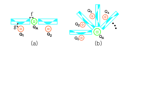
Figure 1: (a) Two qubits $Q_{1}$ and $Q_{2}$ coupled via a bridge qubit $Q_{A}$ in circuit-QED architecture. The coupling between qubit (bridge qubit) and the resonator is $g$ ($f$) at the anti-node of the resonating modes. (b) $n$ qubits coupled via a bridge qubit.

$U_{n}$ is a block-partitioned $(2n+1)\times(2n+1)$ matrix in the basis of $\{|s_{1z},N_{r1},s_{2z},N_{r2},$ $\cdots,s_{nz},N_{rn},s_{az}\rangle\}$. The explicit form of $U_{n}$ for ${\cal N}_{e}=1$ can be calculated as

$$U_{n}=\left(\begin{array}[]{cccccc}Q&T&T&\cdots&T&C\\ T&Q&T&\cdots&T&C\\ T&T&Q&\cdots&T&C\\ \vdots&\vdots&\vdots&\ddots&\vdots&\vdots\\ T&T&T&\cdots&Q&C\\ {C^{\prime}}&C^{\prime}&C^{\prime}&\cdots&C^{\prime}&\frac{\phi^{2}+n\theta^{2}\cos q}{q^{2}}\\ \end{array}\right),$$ (11)

where the matrices $Q,T,C,$ and $C^{\prime}$ are derived in Appendix.

In the transformed Hamiltonian of Eq. (2) the coupling terms in Eq. (II) can be eliminated by introducing the conditions,

$$\tan 2\phi = 2g/\Delta,$$ (12)

$$\tan 2q = \frac{2q(\phi g+n\theta f)}{q^{2}\Delta+n\theta^{2}\Delta^{\prime}},$$ (13)

$$\tan q = \frac{q(\phi f-\theta g)}{\theta\phi\Delta^{\prime}}$$ (14)

with $\Delta\equiv\omega_{q}-\omega_{r}$, $q\equiv\sqrt{\phi^{2}+n\theta^{2}}$, and $\Delta^{\prime}\equiv\omega_{a}-\omega_{q}$, which ensures $[{\tilde{H}}_{n}]_{uv}=0$ if $u+v$=odd. For given $g/\Delta$ and $f/\Delta$, the variables $\phi$, $\theta$, and $\Delta^{\prime}/\Delta$ are determined from these conditions.

As a result, ${\tilde{H}}_{n}$ can be represented as a block-diagonal form,

$${\tilde{H}}_{n}={\tilde{H}}_{n,1}\oplus{\tilde{H}}_{n,2}.$$ (15)

Here ${\tilde{H}}_{n,1}$ is an $n\times n$ matrix whose basis is given by the transformation of $\{|-1/2,N_{r1},-1/2,N_{r2},\cdots,-1/2,$ $N_{rn},-1/2\rangle\}$ by $U_{n}$, describing the resonator modes: one of the resonator modes is excited while all the qubits and bridge qubit are at the ground states. ${\tilde{H}}_{n,2}$ is written by an $(n+1)\times(n+1)$ matrix with the basis obtained by the same transformation of $\{|s_{1z},0,s_{2z},0,$ $\cdots,s_{nz},0,s_{az}\rangle\}$ such as

$${\tilde{H}}_{n,2}=\left(\begin{array}[]{cccccc}e_{q}&j_{q}&j_{q}&\cdots&j_{q}&j_{a}\\ j_{q}&e_{q}&j_{q}&\cdots&j_{q}&j_{a}\\ j_{q}&j_{q}&e_{q}&\cdots&j_{q}&j_{a}\\ \vdots&\vdots&\vdots&\ddots&\vdots&\vdots\\ j_{q}&j_{q}&j_{q}&\cdots&e_{q}&j_{a}\\ j_{a}&j_{a}&j_{a}&\cdots&j_{a}&e_{a}\\ \end{array}\right),$$ (22)

describing the qubit states: one of the qubits or bridge qubit is excited while there is no resonator mode excitation.

The interaction between qubits is described by the Hamiltonian ${\tilde{H}}_{n,2}$. The energy levels of the system of $n$-qubits with a bridge qubit are as follows: for the state with $s_{jz}=1/2$ for only one qubit, $s_{jz}=-1/2$ for other qubits, and $s_{az}=-1/2$, $[{\tilde{H}}_{n,2}]_{ii}=e_{q}$, and for the state with $s_{jz}=-1/2$ for all qubits and $s_{az}=1/2$, $[{\tilde{H}}_{n,2}]_{n+1,n+1}=e_{a}$, where $1\leq i,j\leq n$. The qubit-qubit coupling is given by $[{\tilde{H}}_{n,2}]_{ij}=j_{q}$ for $i\neq j$ and the coupling between a qubit and the bridge qubit by $[{\tilde{H}}_{n,2}]_{i,n+1}=[{\tilde{H}}_{n,2}]_{n+1,j}=j_{a}$. Then, $e_{q}$, $e_{a}$, $j_{q}$, and $j_{a}$ can be explicitly evaluated as

$$j_{q}\!\!\!\! = \!\!\!-\!\frac{1}{2nq^{2}}\!(q^{2}\!\!A\!\!-\!\!\phi^{2}\!B\!\!-\!\!n\theta^{2}\!\!\Delta\!)\!\!+\!\!\frac{\Delta^{\prime}\!\phi^{2}\!\theta^{2}\!\!}{q^{4}}(\!1\!\!-\!\!2\!\sec q\!\!+\!\cos^{2}\!\!q),$$ (23)

$$j_{a}\!\!\! = \!\!\!\frac{\phi\theta}{2q^{2}}(B\!\!-\!\!\Delta)\!\!+\!\!\frac{\Delta^{\prime}\phi\theta}{q^{4}}\![n\theta^{2}\!\!\cos^{2}\!\!q\!\!+\!\!(\phi^{2}\!\!\!-\!\!n\theta^{2})\!\sec q\!-\!\!\phi^{2}],$$ (24)

$$e_{q}\!\!\! = \!\!\!\frac{n-1}{2n}A+\frac{\phi^{2}B-n(q^{2}-\theta^{2})\Delta}{2nq^{2}}$$

$$+\frac{\Delta^{\prime}\phi^{2}\theta^{2}}{q^{4}}(1\!-\!2\sec q\!+\!\cos^{2}q)\!-\!\frac{\omega_{a}}{2}\!+\!\left(1\!-\!\frac{n}{2}\right)\!\omega_{q},$$

$$e_{a}\!\!\! = \!\!\!\frac{n^{2}\theta^{2}}{2nq^{2}}(B\!\!-\!\!\Delta)\!\!+\!\!\frac{\Delta^{\prime}}{q^{4}}(\phi^{4}\!\!+2n\phi^{2}\theta^{2}\sec q+\!n^{2}\theta^{4}\!\cos^{2}q)$$ (26)

$$\!\!\!-\!\frac{\omega_{a}}{2}\!+\!\!\left(\!1\!-\!\frac{n}{2}\!\right)\!\omega_{q},$$

where $A\equiv\Delta\cos 2\phi+2g\sin 2\phi$ and $B\equiv\Delta\cos 2q+(2/q)(n\theta f+\phi g)\sin 2q$.

Further, the coupling term $j_{a}$ between a qubit and the bridge qubit can be eliminated by the transformation,

$$H^{*}_{n,2}={\tilde{U}}^{\dagger}_{n,2}{\tilde{H}}_{n,2}{\tilde{U}}_{n,2},$$ (27)

where

$${\tilde{U}}_{n,2}=e^{\tilde{M}}=e^{-\sum^{n}_{j=1}\eta_{j}(\sigma_{j+}\sigma_{a-}-\sigma_{j-}\sigma_{a+})}.$$ (28)

For the identical qubit case, $\eta_{j}=\eta$, ${\tilde{U}_{n,2}}$ can be explicitly evaluated as before,

$${\tilde{U}}_{n,2}\!\!=\!\!\!\left(\begin{array}[]{ccccc}\!\!\frac{n-1+\cos\sqrt{n}\eta}{n}&\!\!\frac{\cos\sqrt{n}\eta-1}{n}&\!\!\cdots&\!\!\frac{\cos\sqrt{n}\eta-1}{n}&\!\!\!-\frac{\sin\sqrt{n}\eta}{\sqrt{n}}\\ \!\!\frac{\cos\sqrt{n}\eta-1}{n}&\!\!\!\!\!\frac{n-1+\cos\sqrt{n}\eta}{n}&\!\!\cdots&\!\!\frac{\cos\sqrt{n}\eta-1}{n}&\!\!\!-\frac{\sin\sqrt{n}\eta}{\sqrt{n}}\\ \!\!\vdots&\vdots&\!\!\ddots&\vdots&\!\!\!\vdots\\ \!\!\frac{\cos\sqrt{n}\eta-1}{n}&\!\!\frac{\cos\sqrt{n}\eta-1}{n}&\!\!\cdots&\!\!\!\!\frac{n-1+\cos\sqrt{n}\eta}{n}&\!-\!\frac{\sin\!\!\sqrt{n}\eta}{\sqrt{n}}\\ \!\!\frac{\sin\sqrt{n}\eta}{\sqrt{n}}&\!\!\frac{\sin\sqrt{n}\eta}{\sqrt{n}}&\!\!\cdots&\!\!\frac{\sin\sqrt{n}\eta}{\sqrt{n}}&\!\!\!\cos\sqrt{n}\eta\\ \end{array}\!\!\right)\!\!.$$ (34)

By introducing the condition with $\epsilon\equiv e_{a}-e_{q}$,

$$\tan 2\sqrt{n}\eta=\frac{2\sqrt{n}j_{a}}{(n-1)j_{q}-\epsilon},$$ (36)

determining the variable $\eta$, we have

$$H^{*}_{n,2}=\left(\begin{array}[]{cccccc}\varepsilon^{q}_{n}&J_{n}&J_{n}&\cdots&J_{n}&0\\ J_{n}&\varepsilon^{q}_{n}&J_{n}&\cdots&J_{n}&0\\ J_{n}&J_{n}&\varepsilon^{q}_{n}&\cdots&J_{n}&0\\ \vdots&\vdots&\vdots&\ddots&\vdots&\vdots\\ J_{n}&J_{n}&J_{n}&\cdots&\varepsilon^{q}_{n}&0\\ 0&0&0&\cdots&0&\varepsilon^{a}_{n}\end{array}\right).$$ (43)

Here the energy levels are given by

$$\varepsilon^{q}_{n}\!\!\!\! = \!\!\!\frac{1}{n}(\epsilon\!-\!(n\!-\!1)j_{q})\sin^{2}\!\!\!\sqrt{n}\eta\!\!+\!\!\frac{1}{\sqrt{n}}j_{a}\sin 2\!\sqrt{n}\eta\!+\!e_{q},$$ (44)

$$\varepsilon^{a}_{n}\!\!\!\! = \!\!\!\epsilon\!\cos^{2}\!\!\!\!\sqrt{n}\eta\!\!+\!(n\!\!-\!\!1\!)j_{q}\!\sin^{2}\!\!\!\!\sqrt{n}\eta\!-\!\!\sqrt{n}j_{a}\!\sin\!2\!\sqrt{n}\eta\!\!+\!e_{q},$$ (45)

and the qubit-qubit coupling

$$J_{n}\!\! = \!\!\frac{1}{2n}[(n+1)j_{q}+\epsilon+((n-1)j_{q}-\epsilon)\cos 2\sqrt{n}\eta$$ (46)

$$+2\sqrt{n}j_{a}\sin 2\sqrt{n}\eta].$$

This qubit-qubit coupling strength can be explicitly written as

$$J_{n}\!=\!\frac{1}{2n}\!\left[(n+1)j_{q}\!+\!\epsilon+\!\sqrt{((n-1)j_{q}\!-\!\epsilon)^{2}\!+\!4nj_{a}^{2}}\right]$$ (47)

by using the condition of Eq. (36). Here we discard a physically meaningless solution which has a finite value even for $f=0$ or $g=0$.

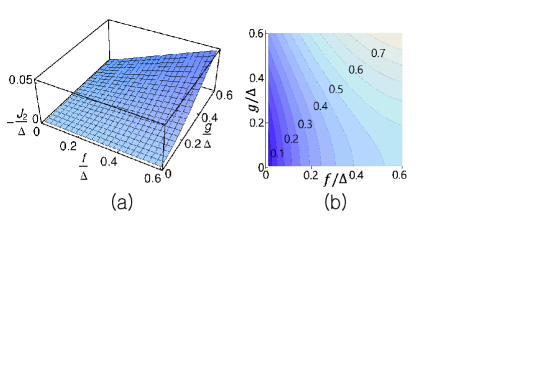
Figure 2: (a) Two qubit xy-coupling $J_{2}$ as a function of $g/\Delta$ and $f/\Delta$. (b) A contour plot for $\Delta^{\prime}/\Delta$ obtained from Eqs. (12)-(14) for $n=2$ in the $(g/\Delta,f/\Delta)$ plane.

The Hamiltonian in Eq. (43) can be represented in the subspace of the Hilbert space satisfying ${\cal N}_{e}=1$ as follows:

$$H^{*}_{n,2}\!=\!\frac{1}{2}\omega^{\prime}_{a}\sigma_{az}\!\!+\!\sum^{n}_{j=1}\frac{1}{2}\omega^{\prime}_{q}\sigma_{jz}\!+\!\!\!\!\sum^{n}_{i,j=1,i\neq j}\!\!\!\!\!\!J_{n}(\sigma_{i+}\sigma_{j-}\!\!+\!\sigma_{i-}\sigma_{j+}).$$

For the state with $s_{az}=-1/2$ and one of $s_{iz}$’s is 1/2 we have $\varepsilon^{q}_{n}=-\frac{(n-2)}{2}\omega^{\prime}_{q}-\frac{1}{2}\omega^{\prime}_{a}$, and for the state with $s_{az}=1/2$ and all $s_{iz}$’s are -1/2 we have $\varepsilon^{a}_{n}=-\frac{n}{2}\omega^{\prime}_{q}+\frac{1}{2}\omega^{\prime}_{a}$, resulting in the relations

$$\omega^{\prime}_{a} = -\frac{1}{n-1}(n\varepsilon^{q}_{n}-(n-2)\varepsilon^{a}_{n}),$$ (49)

$$\omega^{\prime}_{q} = -\frac{1}{n-1}(\varepsilon^{q}_{n}+\varepsilon^{a}_{n}).$$ (50)

Since the Hamiltonian $H^{*}_{n,2}$ with xy-type coupling has the W state as an eigenstate, we can produce the W state in the transformed coordinate with the system of $n$-qubits coupled with each other as shown in Fig. 1(b).

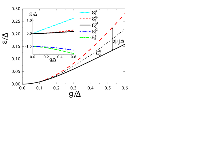
Figure 3: Energy levels of the Hamiltonian ${H}_{2}$ and the two-qubit coupling strength $J_{2}$ for $g=f$. The dotted line shows the energy level, $\varepsilon^{q}_{2}$. In the inset all the energy levels of $H_{2}$ are shown, among which the energy levels, $\varepsilon^{q1}_{2}=\varepsilon^{q}_{2}-|J_{2}|$ and $\varepsilon^{q2}_{2}=\varepsilon^{q}_{2}+|J_{2}|$, are enlarged in the main figure.

III Two-qubit coupling

In this section we will give numerical results of two qubit case ($n=2$). If we set $\omega_{r,1}=\omega_{r,2}=\omega_{r}$ and $\omega_{q,1}=\omega_{q,2}=\omega_{q}$ as before, the transformed Hamiltonian ${\tilde{H}}_{2}=U^{\dagger}_{2}H_{2}U_{2}$ becomes block-diagonalized as

$${\tilde{H}}_{2}={\tilde{H}}_{2,1}\oplus{\tilde{H}}_{2,2}$$ (51)

and we can determine $\Delta^{\prime}/\Delta$, $\phi$, and $\theta$ by using the conditions in Eqs. (12)-(14). As a result, we have

$${\tilde{H}}_{2,2}=\left(\begin{array}[]{ccc}e_{q}&j_{q}&j_{a}\\ j_{q}&e_{q}&j_{a}\\ j_{a}&j_{a}&e_{a}\end{array}\right),$$ (55)

where the basis is given by the transformation of $\{|1/2,0,-1/2,0,-1/2\rangle,|-1/2,0,1/2,0,-1/2\rangle,|-1/2,0,-1/2,0,1/2\rangle\}$ by $U_{2}$. Further, $j_{a}$ term can be eliminated by the transformation $H^{*}_{2,2}={\tilde{U}}^{\dagger}_{2,2}{\tilde{H}}_{2,2}{\tilde{U}}_{2,2}$, and we have

$$H^{*}_{2,2}=\left(\begin{array}[]{ccc}\varepsilon^{q}_{2}&J_{2}&0\\ J_{2}&\varepsilon^{q}_{2}&0\\ 0&0&\varepsilon^{a}_{2}\end{array}\right)$$ (59)

with $\varepsilon^{q}_{2}$, $\varepsilon^{a}_{2}$, and $J_{2}$ in Eqs. (44)-(47).

In Fig. 2(a) we show $J_{2}$ as a function of $g/\Delta$ and $f/\Delta$, where $J_{2}$ increases monotonically from 0 as $g/\Delta$ or $f/\Delta$ increases. Fig. 2(b) shows $\Delta^{\prime}/\Delta$ for obtaining the final Hamiltonian of Eq. (59), which requires that we adjust the value $\Delta^{\prime}/\Delta$ as $g$ or $f$ varies by changing the bridge qubit frequency. If we consider the bridge qubit as a transmon, this can be done by varying the parameter value $E_{J}/E_{C}$ with $E_{J}$ being the Josephson energy and $E_{C}$ the charging energy. In the design of transmon Koch2 the Josephson energy is given by $E_{J}=E_{J,{\rm max}}|\cos(\pi\Phi/\Phi_{0})|$ which can be tuned by the external magnetic flux $\Phi$. From the numerical data of Ref. Koch2, $\delta\omega_{a}$ is tunable such that $\delta\omega_{a}\sim$1GHz for $\delta(E_{J}/E_{C})\sim 10$ around $E_{J}/E_{C}=50$ for a typical transmon Schreier . In Fig. 2(b) $\Delta^{\prime}/\Delta<1$, which can be obtained by adjusting $\delta\Delta^{\prime}\sim\delta\omega_{a}\lesssim$1GHz with $\Delta\approx$1GHz for a circuit-QED architecture Blais .

In the inset of Fig. 3 the eigenvalues of the two-qubit Hamiltonian $H_{2}$ are shown for the case that $g=f$. In the figure $\varepsilon^{r1}_{2}$ and $\varepsilon^{r2}_{2}$ correspond to the energy levels of the resonator modes, and $\varepsilon^{q1}_{2}$, $\varepsilon^{q2}_{2}$, and $\varepsilon^{a}_{2}$ to those of two qubits and bridge qubit, respectively. In Fig. 3 we enlarge the energy levels in the inset corresponding to $\varepsilon^{q1}_{2}$ and $\varepsilon^{q2}_{2}$. Under the unitary transformations, $U_{2}$ and ${\tilde{U}}_{2,2}$, the eigenvalues are invariant, and thus ${\tilde{H}}_{2,1}\oplus H^{*}_{2,2}$ has the same eigenvalues as $H_{2}$. Since from the Hamiltonian $H^{*}_{2,2}$ in Eq. (59) $\varepsilon^{q1}_{2}=\varepsilon^{q}_{2}-|J_{2}|$ and $\varepsilon^{q2}_{2}=\varepsilon^{q}_{2}+|J_{2}|$, we can observe that the energy gap in Fig. 3 is the two-qubit coupling strength which is consistent with the result in Fig. 2(a).

Consider the bridge qubit as the states of transmon at degeneracy point. Then, far from the degeneracy point of the bridge qubit two-qubits can be effectively decoupled, which provides a switching function. In Ref. Majer, a Stark pulse is applied bringing qubits in resonance for a quarter period of oscillation to achieve the $\sqrt{{\rm iSWAP}}$ gate McDermott . In this case two qubits are coupled with the same resonator with the interaction strength $J=g_{1}g_{2}/\Delta$ for the same qubit frequencies, which is derived from the rotating wave approximation and the transformation similar to that in Eq. (3) Blais . In the present case we perform the $\sqrt{{\rm iSWAP}}$ gate similarly by using the switching function: a Stark pulse bring the bridge qubit to degeneracy point and stay for an adjusted time during which two-qubit state evolves. At the end of the $\sqrt{{\rm iSWAP}}$ gate the bridge qubit moves away from the degeneracy point and two-qubit coupling is switched off.

In addition we can consider an one-dimensional qubit array. Owing to the switching function we can selectively choose a pair of nearest neighbor qubits and perform a two-quibt gate, and do the same process for another pair of qubits. In this way we can implement a scalable quantum computing in 1D array of qubits. Moreover, since the qubit-resonator couplings $g$ and $f$ can be tuned by using a three island version of the transmon Gambetta , the two-qubit coupling $J_{n}$ in Eq. (47) can also be in situ controllable. The switching function and controllability is important for scalability of quantum circuit.

IV Discussions and Summary

In section 2 we showed that the W state $|\psi^{\prime*}_{W}\rangle$ can be formed with the coupled qubits in Fig. 1(b) from the Hamiltonian in Eq. (II) in the transformed coordinate. However, this is not the exact W state in the original basis. For the transformed Hamiltonian $H^{*}=U^{\dagger}HU$ with the eigenstate such that $H^{*}|\psi^{\prime*}_{W}\rangle=E|\psi^{\prime*}_{W}\rangle$ the eigenstate $|\psi^{\prime}_{W}\rangle$ of original Hamiltonian $H$ can be calculated as $|\psi^{\prime}_{W}\rangle=U|\psi^{\prime*}_{W}\rangle$.

Actually we have introduced two consecutive transformation, $U_{2}$ and ${\tilde{U}}_{2,2}$, and thus we can obtain $|\psi^{\prime}_{W}\rangle$ represented as $|\psi^{\prime}_{W}\rangle=\sum^{n}_{k=1}(c_{2k-1}|\phi_{2k-1}\rangle+c_{2k}|\phi_{2k}\rangle)+c_{2n+1}|\phi_{2n+1}\rangle$, where the basis ket is given by $\{|s_{1z},N_{r1},s_{2z},N_{r2},$ $\cdots,s_{nz},N_{rn},s_{az}\rangle\}$ as before. For $|\phi_{2k-1}\rangle$ state $N_{rj}=0$ and $s_{az}=s_{jz}=-1/2$ except $s_{kz}=1/2$, for $|\phi_{2k}\rangle$ state $N_{rj}=0$ except $N_{rk}=1$ and $s_{az}=s_{jz}=-1/2$, and for $|\phi_{2n+1}\rangle$ state $N_{rj}=0$, $s_{jz}=-1/2$ and $s_{az}=1/2$, where $1\leq j\leq n$. Here, the coefficients are given by

$$c_{2k-1}\!\!\!\! = \!\!\!\!\frac{1}{\sqrt{n}q^{2}}[(n\theta^{2}\!\!+\!\!\phi^{2}\!\!\cos q)\!\cos\!\!\sqrt{n}\eta\!-\!2\sqrt{n}\phi\theta\!\sin^{2}\!\frac{q}{2}\!\sin\!\!\sqrt{n}\eta],$$

$$c_{2k}\!\!\!\! = \!\!\!\!-\frac{\sin q}{\sqrt{n}q}(\phi\cos\sqrt{n}\eta+\sqrt{n}\theta\sin\sqrt{n}\eta),$$ (60)

$$c_{2n+1}\!\!\!\! = \!\!\!\frac{1}{q^{2}}[(\phi^{2}\!+\!n\theta^{2}\!\cos q)\!\sin\!\sqrt{n}\eta-2\sqrt{n}\phi\theta\!\sin^{2}\!\frac{q}{2}\!\cos\!\sqrt{n}\eta].$$

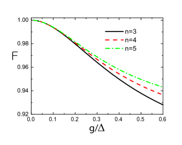
Figure 4: Fidelity for W state formation by using the design in Fig. 1(b) as a function of qubit-resonator coupling strength for $n=3,4,5$.

The fidelity for the W state formation can be given by $F=|\langle\psi_{W}|\psi^{\prime}_{W}\rangle|=(1/\sqrt{n})\sum^{n}_{k=1}c_{2k-1}=\sqrt{n}{\cal C}$ with ${\cal C}=c_{2k-1}$, where $|\psi_{W}\rangle$ is the W state in the original basis. For a tripartite system with $n=3$, for example, $|\psi_{W}\rangle$ is explicitly written as $|\psi_{W}\rangle=(1/\sqrt{3})(|\frac{1}{2},0,-\frac{1}{2},0,-\frac{1}{2},0,-\frac{1}{2}\rangle+|-\frac{1}{2},0,\frac{1}{2},0,$ $-\frac{1}{2},0,-\frac{1}{2}\rangle+|-\frac{1}{2},0,-\frac{1}{2},0,\frac{1}{2},0,-\frac{1}{2}\rangle)$. In superconducting qubit systems the three-qubit W states WKim ; Mlynek have been demonstrated in experiments by using sequential gates Neeley ; Altomare ; Sun . In Fig. 4 the fidelities $F$ are close to 1 for weak coupling, but in this case the gap of energy levels between the W state and the other states become too small. On the other hand, as the coupling increases, the energy gap increases but fidelity decreases. The fidelity increases slightly along with $n$ due to the reduced occupation probability of the bridge qubit state for higher $n$.

The present scheme suffers from the decoherence problem. It is known that decoherence rate increases with the system size Unruh ; Palma . In Fig. 1(a) two qubits and a bridge qubit are coupled to two resonators, which may cause decoherence due to hybridization of the qubits and the cavity. This decoherence effect can be estimated by obtaining the eigenstates of the hybridized system.

From the symmetric eigenstate $|\psi^{*}\rangle_{s}=(1/\sqrt{2})(1~{}1~{}0)^{T}$ of the Hamiltonian $H^{*}_{2,2}$ in Eq. (59) for $n=2$ we obtain the ground state with eigenvalue $\varepsilon^{q1}_{2}$ of the Hamiltonian $H_{2}$ in original basis such as $|\psi\rangle_{g}=c_{1}|\frac{1}{2},0,-\frac{1}{2},0,-\frac{1}{2}\rangle+c_{2}|-\frac{1}{2},1,-\frac{1}{2},0,-\frac{1}{2}\rangle+c_{3}|-\frac{1}{2},0,\frac{1}{2},0,-\frac{1}{2}\rangle+c_{4}|-\frac{1}{2},0,-\frac{1}{2},1,-\frac{1}{2}\rangle+c_{5}|-\frac{1}{2},0,-\frac{1}{2},0,\frac{1}{2}\rangle$, where $c_{i}$’s are given by Eq. (IV) with $n=2$. Also, from the antisymmetric eigenstate $|\psi^{*}\rangle_{a}=(1/\sqrt{2})(1~{}-1~{}0)^{T}$ we have the excited state with eigenvalue $\varepsilon^{q2}_{2}$ such as

$$|\psi\rangle_{e}=\frac{\cos\phi}{\sqrt{2}}|\frac{1}{2},0,-\frac{1}{2},0,-\frac{1}{2}\rangle-\frac{\sin\phi}{\sqrt{2}}|-\frac{1}{2},1,-\frac{1}{2},0,-\frac{1}{2}\rangle$$

$$-\frac{\cos\phi}{\sqrt{2}}|-\frac{1}{2},0,\frac{1}{2},0,-\frac{1}{2}\rangle+\frac{\sin\phi}{\sqrt{2}}|-\frac{1}{2},0,-\frac{1}{2},1,-\frac{1}{2}\rangle.~{}~{}$$ (61)

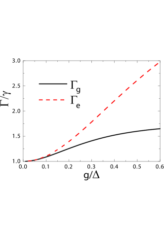
Figure 5: Relaxation rates of the ground and excited states of coupled qubit-resonator system in Fig. 1(a) as a function of qubit-resonator coupling strength. Here we set $\kappa=12\gamma$ Blais1 and $\gamma^{\prime}=\gamma$.

From the eigenstate in original basis we can estimate the decay rate of the ground(excited) state $\Gamma_{g(e)}$ Blais1 as

$$\Gamma_{g} = (c^{2}_{1}+c^{3}_{3})\gamma+(c^{2}_{2}+c^{2}_{4})\kappa+c^{2}_{5}\gamma^{\prime},$$ (62)

$$\Gamma_{e} = \gamma\cos^{2}\phi+\kappa\sin^{2}\phi,$$

where $\gamma$ and $\gamma^{\prime}$ are the relaxation rate of qubit and bridge qubit, respectively, and $\kappa$ that of cavity. Due to coupling to the cavity with large relaxation rate $\kappa>\gamma$ the qubit state decays by the Purcell effect. In Fig. 5 we observe that the relaxation rate of eigenstates increases along with the qubit-resonator coupling $g$. The ratio of relaxation rate of the coupled system to that of the uncoupled qubit remains in the same order for reasonable coupling $g$ so that the present scheme may be viable in real experiments.

In summary, a coupling scheme for qubits in circuit-QED architecture with a bridge qubit introduced between cavities is studied. The cavity modes interacting with the bridge qubit mediate the coupling between qubits. We derive a transformation producing an exact representation of two-qubit coupling for arbitrary number of qubits. Our active coupling scheme enables switching function and control of coupling between qubits. For $n$ qubits coupled with each other the system can produce the W state as an eigenstate of the system. We find that the coupled two-qubit system will be viable in experiments.

Acknowledgments.$-$ This research was supported by Basic Science Research Program through the National Research Foundation of Korea (NRF) funded by the Ministry of Education, Science and Technology (2011-0023467) and by the IT R$\&$D program of MOTIE/KEIT [10043464(2012)].

Appendix A Transformation Matrix

The transformation can be explicitly evaluated for coupled $n$ qubits. Here we, for simplicity, consider identical qubits and resonators, $\phi_{j}=\phi$ and $\theta_{j}=\theta$ and thus

$$U_{n}\!=\!e^{M}\!=\!e^{-\sum^{n}_{j=1}[\phi(a^{\dagger}_{j}\sigma_{j-}-a_{j}\sigma_{j+})+\theta(a^{\dagger}_{j}\sigma_{a-}-a_{j}\sigma_{a+})]}.$$ (63)

Then, the $U_{n}$ can be represented as a block-partitioned $(2n+1)\times(2n+1)$ matrix consisting of $Q,T,C$ and $C^{\prime}$ for ${\cal N}_{e}=1$ as shown in Eq. (11). If we expand $U_{n}$ by using the relation, $e^{M}=1+M+\frac{1}{2!}M^{2}+\frac{1}{3!}M^{3}+\cdot\cdot\cdot$, we obtain

$$Q_{11} = 1+\phi^{2}\sum^{\infty}_{m=1}\frac{(-1)^{m}}{(2m)!}a_{m}$$ (64)

$$Q_{22} = \sum^{\infty}_{m=1}\frac{(-1)^{m-1}}{(2m-2)!}a_{m}$$ (65)

$$Q_{12} = \phi\sum^{\infty}_{m=1}\frac{(-1)^{m-1}}{(2m-1)!}a_{m}$$ (66)

$$Q_{21} = -Q_{12}$$ (67)

with

$$a_{1} = 1,$$

$$a_{2} = \phi^{2}+\theta^{2},$$

$$a_{3} = \phi^{4}+2\phi^{2}\theta^{2}+n\theta^{4},$$ (68)

$$a_{4} = \phi^{6}+3\phi^{4}\theta^{2}+3n\phi^{2}\theta^{4}+n^{2}\theta^{6},$$

$$\cdots$$

This series has the following general form

$$a_{m} = q^{2(m-1)}-(n-1)\theta^{2}\sum^{m-1}_{l=1}q^{2(m-l-1)}\phi^{2(l-1)}$$ (69)

$$= \frac{1}{n}q^{2(m-1)}+\frac{n-1}{n}\phi^{2(m-1)}$$

with $q=\sqrt{\phi^{2}+n\theta^{2}}$ and thus the matrix $Q$ can be written as

$$Q=\left(\begin{array}[]{cc}\frac{\phi^{2}}{nq^{2}}\cos q+\frac{n-1}{n}\cos\phi+\frac{\theta^{2}}{q^{2}}&\frac{\phi}{nq}\sin q+\frac{n-1}{n}\sin\phi\\ -\frac{\phi}{nq}\sin q-\frac{n-1}{n}\sin\phi&\frac{1}{n}\cos q+\frac{n-1}{n}\cos\phi\\ \end{array}\right).$$ (72)

For the matrix $T$ we have similar results such that

$$T_{11} = \phi^{2}\sum^{\infty}_{m=1}\frac{(-1)^{m+1}}{(2m+2)!}b_{m}$$ (74)

$$T_{22} = \sum^{\infty}_{m=1}\frac{(-1)^{m}}{(2m)!}b_{m}$$ (75)

$$T_{12} = \phi\sum^{\infty}_{m=1}\frac{(-1)^{m}}{(2m+1)!}b_{m}$$ (76)

$$T_{21} = -T_{12}$$ (77)

with

$$b_{1} = \theta^{2},$$

$$b_{2} = \theta^{2}(2\phi^{2}+n\theta^{2}),$$

$$b_{3} = \theta^{2}(3\phi^{4}+3n\phi^{2}\theta^{2}+n^{2}\theta^{4}),$$ (78)

$$b_{4} = \theta^{2}(4\phi^{6}+6n\phi^{4}\theta^{2}+4n^{2}\phi^{2}\theta^{4}+n^{3}\theta^{6}),$$

$$\cdots$$

and thus

$$b_{m} = \frac{1}{n}\left(q^{2m}-\phi^{2m}\right),$$ (79)

resulting in

$$T=\left(\begin{array}[]{cc}\frac{\phi^{2}}{nq^{2}}\cos q-\frac{1}{n}\cos\phi+\frac{\theta^{2}}{q^{2}}&\frac{\phi}{nq}\sin q-\frac{1}{n}\sin\phi\\ -\frac{\phi}{nq}\sin q+\frac{1}{n}\sin\phi&\frac{1}{n}\cos q-\frac{1}{n}\cos\phi\\ \end{array}\right).$$ (82)

The elements of matrices $C$ and $C^{\prime}$ also can be evaluated similarly as

$$C_{1} = -\frac{1}{2!}\phi\theta+\frac{1}{4!}\phi\theta(\phi^{2}+n\theta^{2})-\frac{1}{6!}\phi\theta(\phi^{2}+n\theta^{2})^{2}+\cdots$$

$$C_{2} = -\theta+\frac{1}{3!}\theta(\phi^{2}+n\theta^{2})-\frac{1}{5!}\theta(\phi^{2}+n\theta^{2})^{2}+\cdots$$

$C^{\prime}_{1}=C_{1}$, and $C^{\prime}_{2}=-C_{2}$, resulting in

$$C = \left(\begin{array}[]{c}\frac{\phi\theta}{q^{2}}(\cos q-1)\\ -\frac{\theta}{q}\sin q\\ \end{array}\right),$$ (88)

$$C^{\prime} = \left(\begin{array}[]{cc}\frac{\phi\theta}{q^{2}}(\cos q-1)&\frac{\theta}{q}\sin q\\ \end{array}\right).$$ (90)

Finally, the matrix element, $[U_{n}]_{2n+1,2n+1}$, can be evaluated as

$$[U_{n}]_{2n+1,2n+1} = 1-\frac{1}{2!}n\theta^{2}+\frac{1}{4!}n\theta^{2}(\phi^{2}+n\theta^{2})-\cdots$$ (91)

$$= \frac{\phi^{2}+n\theta^{2}\cos q}{q^{2}}.$$

References

- (1) A. Blais, R.-S. Huang, A. Wallraff, S. M. Girvin, and R. J. Schoelkopf, Phys. Rev. A 69, 062320 (2004).
- (2) A. Blais, J. Gambetta, A. Wallraff, D. I. Schuster, S. M. Girvin, M. H. Devoret, and R. J. Schoelkopf, Phys. Rev. A 75, 032329 (2007).
- (3) J. Majer, J. M. Chow, J. M. Gambetta, J. Koch, B. R. Johnson, J. A. Schreier, L. Frunzio, D. I. Schuster, A. A. Houck, A. Wallraff, A. Blais, M. H. Devoret, S. M. Girvin, and R. J. Schoelkopf, Nature 449, 443 (2007).
- (4) L. DiCarlo, J. M. Chow, J. M. Gambetta, Lev S. Bishop, B. R. Johnson, D. I. Schuster, J. Majer, A. Blais, L. Frunzio, S. M. Girvin, and R. J. Schoelkopf, Nature 460, 240 (2009).
- (5) A. F. van Loo, A. Fedorov, K. Lalumiere, B. C. Sanders, A. Blais, and A. Wallraff, Science 342, 1494 (2013).
- (6) M. D. Kim, Quantum Inf. Proc. 14, 3677 (2015).
- (7) M. D. Reed, L. DiCarlo, S. E. Nigg, L. Sun, L. Frunzio, S. M. Girvin, and R. J. Schoelkopf, Nature 482, 382 (2012).
- (8) S. Schmidt and J. Koch, Ann. Phys. 525, 395 (2013).
- (9) A. A. Houck, H. E. Türeci, and J. Koch, Nature Phys. 8, 292 (2012).
- (10) D. L. Underwood, W. E. Shanks, J. Koch, and A. A. Houck, Phys. Rev. A 86, 023837 (2012).
- (11) M. Leib and M. J. Hartmann, New J. Phys. 12, 093031 (2010).
- (12) S. Schmidt, D. Gerace, A. A. Houck, G. Blatter, and H. E. Türeci, Phys. Rev. B 82, 100507(R) (2010).
- (13) L. Tian, Phys. Rev. Lett. 105, 167001 (2010).
- (14) J. Koch, A. A. Houck, K. Le Hur, and S. M. Girvin, Phys. Rev. A 82, 043811 (2010).
- (15) A. Nunnenkamp, J. Koch, and S. M. Girvin, New J. Phys. 13, 095008 (2011).
- (16) F. W. Strauch, K. Jacobs, and R. W. Simmonds, Phys. Rev. Lett. 105, 050501 (2010).
- (17) F. W. Strauch, D. Onyango, K. Jacobs, and R. W. Simmonds, Phys. Rev. A 85, 022335 (2012).
- (18) R. Sharma and F. W. Strauch, arXiv:1503.02157 [quant-ph].
- (19) M. Sandberg, D. Mcclure, H. Paik, D. F. Bogorin, B. L. T. Plourde, O. Dial, B. Abdo, unpublished (http://meetings.aps.org/link/BAPS.2015.MAR.B39.11).
- (20) J. Koch, T. M. Yu, J. Gambetta, A. A. Houck, D. I. Schuster, J. Majer, A. Blais, M. H. Devoret, S. M. Girvin, and R. J. Schoelkopf, Phys. Rev. A 76, 042319 (2007).
- (21) J. A. Schreier, A. A. Houck, Jens Koch, D. I. Schuster, B. R. Johnson, J. M. Chow, J. M. Gambetta, J. Majer, L. Frunzio, M. H. Devoret, S. M. Girvin, and R. J. Schoelkopf, Phys. Rev. B 77, 180502(R) (2008).
- (22) R. McDermott, R. W. Simmonds, M. Steffen, K. B. Cooper, K. Cicak, K. D. Osborn, S. Oh, D. P. Pappas, J. M. Martinis, Science 307, 1299 (2005).
- (23) J. M. Gambetta, A. A. Houck, and A. Blais, Phys. Rev. Lett. 106, 030502 (2011).
- (24) M. D. Kim and S. Y. Cho, Phys. Rev. B 77, 100508(R) (2008).
- (25) J. A. Mlynek, A. A. Abdumalikov, Jr., J. M. Fink, L. Steffen, M. Baur, C. Lang, A. F. van Loo, and A. Wallraff, Phys. Rev. A 86, 053838 (2012).
- (26) M. Neeley, R. C. Bialczak, M. Lenander, E. Lucero, M. Mariantoni, A. D. O Connell, D. Sank, H. Wang, M. Weides, J. Wenner, Y. Yin, T. Yamamoto, A. N. Cleland, and J. M. Martinis, Nature 467, 570 (2010).
- (27) F. Altomare, J. I. Park, K. Cicak, M. A. Sillanpaa, M. S. Allman, D. Li, A. Sirois, J. A. Strong, J. D. Whittaker, and R.W. Simmonds, Nature Phys. 6, 777 (2010)
- (28) G. Sun, X. Wen, B. Mao, J. Chen, Y. Yu, P. Wu, and S. Han, Nature Comm. 1, 51 (2012).
- (29) W. G. Unruh, Phys. Rev. A 51 992 (1995).
- (30) G. M. Palma, K. A. Suominen, and A. K. Ekert, Proc. R. Soc. London A 452, 567 (1996).