Absorption lines from magnetically-driven winds in X-ray binaries

Abstract

Context. High resolution X-ray spectra of black hole X-ray binaries (BHBs) show blueshifted absorption lines suggesting presence of outflowing winds. Further, observations show that the disk winds are equatorial and they occur in the Softer (disk-dominated) states of the outburst and are less prominent or absent in the Harder (power-law dominated) states.

Aims. We want to test if the self-similar magneto-hydrodynamic (MHD) accretion-ejection models can explain the observational results for accretion disk winds in BHBs. In our models, the density at the base of the outflow from the accretion disk is not a free parameter. This mass loading is determined by solving the full set of dynamical MHD equations without neglecting any physical term. Thus the physical properties of the outflow depend on and are controlled by the global structure of the disk.

Methods. We studied different MHD solutions characterized by different values of (a) the disk aspect ratio ($\varepsilon$) and (b) the ejection efficiency ($p$). We also generate two kinds of MHD solutions depending on the absence (cold solution) or presence (warm solution) of heating at the disk surface. Such heating could be from e.g. dissipation of energy due to MHD turbulence in the disk or illumination. Warm solutions can have large ($>0.1$) values of $p$ which would imply larger wind mass loading at the base of the outflow. We use each of these MHD solutions to predict the physical parameters (e.g. distance density, velocity, magnetic field etc.) of an outflow. We have put limits on the ionization parameter ($\xi$), column density and timescales, motivated by observational results. Further constraints were derived for the allowed values of $\xi$ from thermodynamic instability considerations, particularly for the Hard SED. These physical constraints were imposed on each of these outflows to select regions within it, which are consistent with the observed winds.

Results. The cold MHD solutions are found to be inadequate to account for winds due to their low ejection efficiency. On the contrary warm solutions can have sufficiently high values of $p(\gtrsim 0.1)$ which is required to explain the observed physical quantities in the wind. From our thermodynamic equilibrium curve analysis for the outflowing gas, we found that in the Hard state a range of $\xi$ is unstable. This constrain makes it impossible to have any wind at all, in the Hard state.

Conclusions. Using the MHD outflow models we could explain the observed trends - that the winds are equatorial and that they are observable in the Soft states (and not expected in the Hard state) of the BHB outbursts.

1 Introduction

The launch of Chandra and XMM-Newton, revealed blueshifted absorption lines in the high resolution X-ray spectra of stellar mass black holes in binaries (BHBs). These are signatures of winds from the accretion disk around the black hole. The velocity and ionization state of the gas, interpreted from the absorption lines, vary from object to object and from observation to observation. In most cases, only H- and He-like Fe ions are detected (e.g Lee et al. 2002, Neilsen & Lee 2009 for GRS 1915+105, Miller et al. 2004 for GX 339-4, Miller et al. 2006 for H1743-322 and King et al. 2012 for IGR J17091-3624). In some of the objects however, a wider range of ions is seen from O through Fe (e.g. Ueda et al. 2009 for GRS 1915+105, Miller et al. 2008; Kallman et al. 2009 for GRO J1655–40). The variations in the wind properties seem to indicate variations in the temperature, pressure and density of the gas from one object to another. Further, even in the same object, the winds seem to have variations depending on the accretion state of the black hole.

Both spectral and timing observations of most BHBs show common behaviour patterns centered around a few states of accretion. The spectral energy distributions (SEDs) corresponding to the different states have varying degree of contribution from the accretion disk and the non-thermal power-law components. The X-ray studies of BHB show that winds are not present in all states. It has been shown by several authors that the absorption lines are more prominent in the Softer (accretion disk dominated) states (Miller et al. 2008; Neilsen & Lee 2009; Blum et al. 2010; Ponti et al. 2012). For some objects, the reason for such changes is attributed to changes in the photoionizing flux (e.g. Miller et al. 2012, in the case of H1743-322). However, the alternative explanation of ‘changes in the driving mechanism’ is of greater relevance to this paper.

The observable properties of the accretion disk winds are often used to infer the driving mechanism of the winds (Lee et al. 2002; Ueda et al. 2009, 2010; Neilsen et al. 2011; Neilsen & Homan 2012). Hence the variation or disappearance of the wind through the various states of the BHB, has been interpreted as variation in the driving mechanism of the wind. A good example is the case of GRO J1655–40. A well known Chandra observation of GRO J1655–40 (Miller et al. 2006, 2008; Kallman et al. 2009), showed a rich absorption line spectrum from OVIII - NiXXVI, and led the authors to conclude for magnetic driving mechanism for the wind. Neilsen & Homan (2012) analysed the data from another observation from 3 weeks later, for the same source, and found absorption by Fe  xxvi only. They argue that such a change cannot be due to variation in photoionization flux only and suggest that variable thermal pressure and magnetic fields may be important in driving long-term changes in the wind in GRO J1655–40.

To get a consolidated picture of these systems, it is necessary to understand the relation between the accretion states of the BHBs and the driving mechanisms of the winds. In this paper we investigate the magneto hydrodynamic (hereafter MHD) solutions as driving mechanisms for winds from the accretion disks around BHBs - cold solutions from Ferreira (1997, hereafter F97) and warm solutions from Casse & Ferreira (2000b) and Ferreira (2004). To understand the basic motivation of the MHD solutions used to model the winds, throughout this paper, it is important to discuss the distinction between winds and jets from accretion disks. Observationally, jets are usually described as collimated, fast (mildly relativistic) outflows detected or directly imaged in radio wavelengths. On the other hand, winds are detected as absorption features, showing speeds of a few thousand $\rm{km\,s^{-1}}$. However, on the theoretical side, both are outflows launched from the accretion disk surface due to magnetic and/or thermal/radiative effects. The power carried by these outflows is, ultimately, a fraction of the released accretion power. Hence, although observationally distinct, theoretically, it is not simple to distinguish between the two. One way to make a clear theoretical distinction between these two outflows is to look at the magnetization $\sigma$ at the disk surface, namely the ratio of the MHD Poynting flux to the sum of the thermal energy flux and the kinetic energy flux. Jets would have $\sigma>1$, a high magnetization translating into both large asymptotic speeds and (magnetic) self-confinement. On the contrary, winds would be much less magnetized ($\sigma<1$) with much lower asymptotic speeds and the confinement (if any) will come only from the external medium.

MHD solutions have been used by other authors to address outflows in various systems. Of particular relevance to this paper are the works presented by Fukumura et al. (2010a, b, 2014, 2015). Based on the self-similar Contopoulos & Lovelace (1994) MHD models of outflowing material, the aforementioned papers have already argued in favour of large scale magneto-centrifugally driven winds in active galactic nuclei (AGN - galaxies which host actively mass accreting super-massive, $M_{BH}>10^{6}M_{\odot}$, black holes at their centres). Their analysis shows that such models can account for the observed warm absorbers and ultra-fast outflows seen as absorption lines in high resolution X-ray spectra of AGN. They have also attempted to explain the broad absorption lines (seen in high resolution ultraviolet spectra of AGN) using the same MHD wind models. Note however, that the Contopoulos & Lovelace (1994) model (which is an extension of the Blandford & Payne 1982 hydromagnetic flows ) does not treat the underlying disk. As a consequence, the link between the mass loss in winds and the disk accretion rate is lost and the mass loading at the base of the disk can be (almost) arbitrarily large or small. On the contrary, the MHD models in F97 (and subsequent papers) link the density of the outflowing material to the disk accretion rate.

A consistent theory of MHD outflows from the disk must explain how much matter from the disk is deviated from the radial to the vertical motion, as well as the amount of energy and angular momentum carried away from the disk. This requires a thorough treatment of the resistive disk interior and matching it with the outflowing material using ideal MHD. The only way to solve such an entangled problem is to take into account all dynamical terms, a task that has been done within a self-similar framework in F97.

The F97 MHD solutions have been used in Ferreira et al. (2006) and Petrucci et al. (2010), to describe accretion disks giving rise to jets in the Hard States of BHBs. Winds, on the other hand are seen in the Soft state of the BHBs when radio jets are absent. Using the F97 models we aim to test if the same theoretical framework (which could reproduce jets) can reproduce the observed properties of the winds (ionization parameter, column density, velocity etc.). We shall further, look into the parameter space of the theoretical models to distinguish between the Softer accretion states, when the wind is observed and the Harder states when the absorption lines from the wind is not observed.

2 The MHD accretion disk wind solutions

2.1 General properties

We use the F97 solutions describing steady-state, axisymmetric solutions under the following two conditions:
(1) A large scale magnetic field of bipolar topology is assumed to thread the accretion disk. The strength of the required vertical magnetic field component is obtained as a result of the solution (Ferreira 1995).
(2) Some anomalous turbulent resistivity is at work, allowing the plasma to diffuse through the field lines inside the disk.

For a set of disk parameters, the solutions are computed from the disk midplane to the asymptotic regime, the outflowing material becoming, first, super slow-magnetosonic, then, Alfvénic and finally, fast-magnetosonic. All solutions that will be discussed in this paper, have this same asymptotic behavior which corresponds to the following physical scenario: after an opening of the radius of the outflow, leading to a very efficient acceleration of the plasma, the outflow undergoes a refocusing towards the axis (recollimation). The solutions are then, mathematically terminated (see F97 for more details). Physically speaking however, the outflowing plasma will most probably undergo an oblique shock (which is independent of the assumption concerning the thermal state of the magnetic surfaces) after the recollimation happens. However, theoretically accounting for the oblique shock is beyond the scope of this paper. Thus, in this paper we rely on those solutions only, which cross their Alfvén surfaces before recollimating (i.e. before the solutions have to be mathematically terminated).

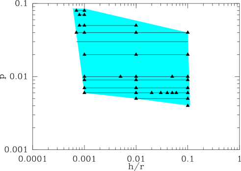
Figure 1: Parameter space ejection index $p$ ($\dot{M}_{acc}\propto r^{p}$) versus disk aspect ratio $\varepsilon=h/r$ for isothermal, cold accretion-ejection solutions of F97. The colored area shows the zone where super-Alfvenic outflows have been obtained, the triangles are some specific solutions and lines are for constant $p$.

2.2 Model parameters

The rigorous mathematical details of how the isothermal MHD solutions for the accretion disk outflow are obtained are given in the aforementioned papers and we refrain from repeating them here. In this section, we focus on describing the two parameters that affect the density $n^{+}$ (or $\rho^{+}$) of the outflowing material at a given radius $r$ in the disk.

Because of ejection, the disk accretion rate varies with the radius even in a steady state, namely $\dot{M}_{acc}\propto r^{p}$. This radial exponent, $p$ (labelled $\xi$ in F97, Ferreira et al. 2006; Petrucci et al. 2010, etc.) is very important since it measures the local ejection efficiency. For an accretion disk which is giving rise to an outflow, the mass outflow rate is related to the accretion rate through the ejection index p. If the disk extends between the inner radius $r_{in}$ and the outer radius $r_{out}$ and is being fed by a disc accretion rate $\dot{M}_{acc}(r_{out})$, the ejection to accretion mass rate ratio is

$$\frac{2\dot{M}_{outflow}}{\dot{M}_{acc}(r_{out})}=1-\left(\frac{r_{in}}{r_{out}}\right)^{p}\simeq p\ln\frac{r_{out}}{r_{in}}$$ (1)

where the last estimate holds only for $p<<1$. For the most extreme MHD solution discussed in this paper (namely $r_{out}\simeq 10^{7}r_{in}$ and $p\simeq 0.1$), about 80% of the accreted mass is ejected in the form of the outflow. The larger the exponent, the more massive and slower is the outflow. Mass conservation writes

$$2\frac{d\dot{M}_{outflow}}{dr}=4\pi r\rho^{+}u^{+}_{z} = \frac{d\dot{M}_{acc}}{dr}=p\frac{\dot{M}_{acc}}{r}$$

$$n^{+}m_{p}=\rho^{+} \simeq \frac{p}{\varepsilon}\frac{\dot{M}_{acc}}{4\pi\Omega_{K}r^{3}}$$ (2)

where $m_{p}$ is the proton mass and the superscript ”+” stands for the height where the flow velocity becomes sonic, namely $u_{z}^{+}=C_{s}=\Omega_{K}h=\varepsilon V_{K}$. Here, $V_{K}=\Omega_{K}r=\sqrt{GM_{BH}/r}$ ($G$: gravitational constant) is the keplerian speed and

$$\varepsilon=\frac{h}{r}$$ (3)

is the disk aspect ratio, where $h(r)$ is the vertical scale height at the cylindrical radius $r$. It can thus be seen that the wind density, a crucial quantity when studying absorption features, is mostly dependent on $p$ and $\varepsilon$ for a given disk accretion rate $\dot{M}_{acc}$.

Equation 2 is the fundamental difference between the MHD models used in the aforementioned papers by Fukumura et al. and the ones used in this work. While in the former, the initial wind density $\rho^{+}$ can be “arbitrarily” prescribed i.e. independent of the the underlying disk accretion rate, here it is a result of an accretion-ejection calculation and are determined by $p$ and $\varepsilon$. In the Fukumura et al. papers there are two assumptions, put by hand, that determine the physical properties of the outflow. a) The authors do not use the parameter $p$. However, comparing the equations for the radial distributions of magnetic field ($B_{z}\propto r^{q-2}$) of the outflow, we can get the relation $q=\frac{3}{4}+\frac{p}{2}$ (Ferreira 1993). Note that $q$ is not any parameter related to the accretion disk, but an index related to the outflow. The Fukumura et al. papers discuss the two cases of with $q=1$ and $q=3/4$, but for modelling the AGN winds they use the former, which would correspond to $p=0.5$. The choice of $q=1$ was to ensure that the density in the outflow followed $n\propto r^{\alpha}$ with $\alpha=2q-3=1$, as suggested by observations. b) The density at the launching point of the wind is prescribed by a parameter $\eta_{W}$ which is the ratio of the mass outflow rate to the disk accretion rate. Note that the authors use a constant value $\eta_{W}=0.5$, independent of $q$. These preassigned values for the parameters defining the outflow and the lack of any connection to the accretion process, fosters a sense of ”physical arbitrariness”. To achieve such a high value of $\eta_{W}$, an extra process (other than magneto-hydrodynamic acceleration) must be acting within the resistive disk (this will be discussed later in Section 5 in the context of “Warm” models).

In the MHD models used in this paper the value of the exponent $p$ influences the extent of magnetisation in the outflow. This is another way in which the ejection index relates the accretion process and the outflow properties. In a non-relativistic framework the ratio of the MHD Poynting flux to the kinetic energy flux at the disk surface is

$$\sigma^{+}\simeq\frac{1}{p}\left(\frac{\Lambda}{1+\Lambda}\right)$$ (4)

(F97, Casse & Ferreira 2000a) where $\Lambda$ is the ratio of the torque due to the outflow to the turbulent torque (usually referred to as the viscous torque). The torque due to the outflow transfers the disk angular momentum to the outflowing material whereas the turbulent torque provides an outward radial transport within the disk. Smaller the value of $p$, larger is the energy per unit mass in the outflow. A magnetically dominated self-confined outflow requires $\sigma^{+}>1$. The F97 outflow models have been obtained in the limit $\Lambda\rightarrow\infty$ so that the self-confined outflows carry away all the disk angular momentum and thereby rotational energy with $\sigma^{+}\simeq 1/p\gg 1$. The outflow material reaches the maximum asymptotic poloidal speed $V_{max}\sim V_{K}(r_{o})p^{-1/2}$, where $r_{o}$ is the anchoring radius of the magnetic field line.

Figure 1 shows the $p-\varepsilon$ parameter space of super-Alfvenic MHD solutions obtained by F97 with cold, isothermal magnetic surfaces. It can be seen that under these assumptions it is impossible to achieve high values of $p\gtrsim 0.1$. Such a limit on the value of $p$ does not improve even if the magnetic surfaces are changed to be adiabatic, as long as the outflowing material remains cold (Casse & Ferreira 2000a). The outflow is cold when its enthalpy is negligible when compared to the magnetic energy, which is always verified in near Keplerian accretion disks. However, the warming up of the outflowing material could occur if some additional heat deposition becomes active at the disk surface layers (through illumination for instance, or enhanced turbulent dissipation at the base of the corona). In that case, larger values of $p$ up to $\sim 0.45$ have been reported (Casse & Ferreira 2000b; Ferreira 2004). We will examine the cold outflows in Section 4 and the “warm outflows” in Section 5.

2.3 The scaling relationships

For the MHD outflow (with given $\varepsilon$ and $p$) emitted from the accretion disk settled around a black hole, the important physical quantities are given at any cylindrical (r,z) by

$$n(r,z)=\frac{\dot{m}}{\sigma_{T}r_{g}}\left(\frac{r}{r_{g}}\right)^{(p-3/2)}f_{n}(y)$$ (5)

$$B_{i}(r,z)=\left(\frac{\mu_{o}m_{p}\dot{m}c^{2}}{\sigma_{T}r_{g}}\right)^{1/2}\left(\frac{r}{r_{g}}\right)^{(-5/4+p/2)}f_{B_{i}}(y)$$ (6)

$$v_{i}(r,z) = c\left(\frac{r}{r_{g}}\right)^{-1/2}f_{v_{i}}(y)$$ (7)

$$\tau_{dyn}(r) = \frac{2\pi r_{g}}{c}\left(\frac{r}{r_{g}}\right)^{3/2}f_{\tau}(y)$$ (8)

where $\sigma_{T}$ is the Thomson cross section, $c$ the speed of light, $r_{g}=GM_{BH}/c^{2}$ is the gravitational radius, $\mu_{o}$ the vacuum magnetic permeability, $y=z/r$ the self-similar variable and the functions $f_{X}(y)$ are provided by the solution of the full set of MHD equations. In the above expressions, $n$ is the proton number density and we consider it to be $\sim n_{H}$ (the Hydrogen number density); $v_{i}$ (or $B_{i}$) is any component of the velocity (or magnetic field) and $\tau_{dyn}=1/div\bf{V}$ (where $\bf{V}$ is the plasma velocity) is a measure of the dynamical time in the flow. The normalized disk accretion rate used in the above equations is defined by

$$\dot{m}=\frac{\dot{M}_{acc}(r_{g})\,c^{2}}{L_{Edd}}$$

where $L_{Edd}$ is the Eddington luminosity.

Note that we are using a steady state assumption for the accretion disk of a BHB i.e. the variation of the accretion rate with the radius is assumed to be the same for the entire disk (same $p$ and same normalization). This assumption is maintained from the innermost regions (a few $r_{g}$) to the outer part of the disk where the disk wind becomes relevant (between $10^{3}-10^{4}r_{g}$). We acknowledge that this is a simplistic picture since BHBs are outbursting systems where the accretion rate is obviously varying. So the accretion rate of the outer part of disk could be significantly different to the one in the inner part. Taking this effect into account would however, require considering a detailed time evolution of the accretion mechanism through the different stages of the outburst which is far beyond the scope of this paper. Hence we proceed forward to perform our calculations, within the aforementioned scientific framework.

3 Observational constrains

3.1 The spectral energy distribution for the Soft and the Hard state

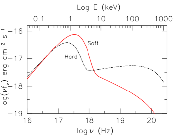
Figure 2: The SEDs corresponding to the Soft and Hard states of the outburst of a black hole of $10M_{\odot}$. The two important components of the SED, namely, the disk spectrum and the power-law have been added following the scheme described in Remillard & McClintock (2006). See Section 3.1 for the details.

The SED of BHBs usually comprises of two components - (1) a thermal component and (2) a non thermal power-law component with a photon spectrum $N(E)\propto E^{-\Gamma}$ (Remillard & McClintock 2006). The thermal component is believed to be the radiation from the inner accretion disk around the black hole, and is conventionally modeled with a multi-temperature blackbody often showing a characteristic temperature ($T_{in}$) near 1 keV. During their outbursts the BHBs transition through different states where the SED shows varying degrees of contribution from the aforementioned components. The state where the radiation from the inner accretion disk dominates and contributes more than 75% of the 2-20 keV flux, is fiducially called the Soft state (Remillard & McClintock 2006). On the other hand the fiducial Hard state is one when the non thermal power-law contributes more than 80% of the 2-20 keV flux (Remillard & McClintock 2006). For any given BHB, the accretion disk usually appears to be fainter and cooler in this Hard power-law state than it is in the Soft thermal state.

The radiation from a thin accretion disk may be modeled as the sum of local blackbodies emitted at different radii and the temperature $T_{in}$ of the innermost annulus (with radius $r_{in}$) of accreted matter is proportional to $\left[\dot{m}_{obs}/(M_{BH}r_{in}^{3})\right]^{1/4}$ (Peterson 1997; Frank, King & Raine 2002) where the observational accretion rate $\dot{m}_{obs}$ is defined as

$$\dot{m}_{obs}=L_{rad}/L_{Edd},$$ (9)

$L_{rad}$ being the luminosity in the energy range 0.2 to 20 keV and $L_{Edd}$ being the Eddington luminosity. A standard model for emission from a thin accretion disk is available as disk blackbody (hereafter diskbb, Mitsuda et al. 1984; Makishima et al. 1987) in XSPEC (Arnaud 1996). We use the diskbb in version 11.3 of XSPEC to generate the disk spectrum $f_{disk}(\nu)$, where $T_{in}$ is used as an input. The other required input for diskbb, the normalisation, is proportional to $r_{in}^{2}$. To $f_{disk}(\nu)$ we add a hard power-law with a high energy cut-off, yielding

$$f(\nu)=f_{disk}(\nu)+[A_{pl}\nu^{-\alpha}]\exp{{}^{-\frac{\nu}{\nu_{max}}}}$$ (10)

to account for the full SED. We use the high energy exponential cut-off to insert a break in the power-law at 100 keV.

We follow the prescription given in Remillard & McClintock (2006) to choose appropriate values of the relevant parameters to derive the two representative SEDs for a black hole of $10M_{\odot}$.

1. Soft state (Figure 2 solid red curve): In the Soft state the accretion disk extends all the way to $r_{in}=3R_{s}=6r_{g}$. Thus $T_{in}=0.56\,{\rm keV}$. The power-law has $\Gamma=2.5$ and $A_{pl}$ is chosen in such a way that disk contributes to 80% of the 2-20 keV flux.

2. Hard state (Figure 2 dotted-and-dashed black curve): With $r_{in}=6R_{s}=12r_{g}$ we generate a cooler disk with $T_{in}=0.33\,{\rm keV}$. The power-law is dominant in this state with $\Gamma=1.8$ so that 2-20 keV flux is only 20%.

For a $10M_{\odot}$ black hole, $L_{Edd}=1.23\times 10^{39}\rm{erg\,s^{-1}}$. Using the aforementioned fiducial SEDs, we can derive $\dot{m}_{obs}=0.14$ using the Soft SED and is equal to $0.07$ for the Hard SED. Thus for simplicity we assume $\dot{m}_{obs}=0.1$ for the rest of this paper.

It is important to note here, the distinction between the disk accretion rate $\dot{m}$ (Equations 5 and 2.3) mentioned above, and the observed accretion rate $\dot{m}_{obs}$ which is more commonly used in the literature. One can define,

$$\dot{m}=\frac{2}{\eta_{acc}}\frac{\dot{m}_{obs}}{\eta_{rad}}$$ (11)

where the factor $2$ is due to the assumption that we see only one of the two surfaces of the disk.

The accretion efficiency $\eta_{acc}\simeq r_{g}/2r_{in}$ depends mostly on the black hole spin. For the sake of simplicity, we choose the Schwarzchild black hole, so that $\eta_{acc}\sim 1/12$, both in Soft and Hard state.

The radiative efficiency, $\eta_{rad}=1$ if the inner accretion flow is radiatively efficient i.e. it radiates away all the power released due to accretion. This is the case for a standard (i.e. geometrically thin, optically thick) accretion disk and is satisfied in the Soft state when the standard accretion disk extends all the way up to $r_{in}=6r_{g}$. Thus $\dot{m}=24\dot{m}_{obs}=2.4$. We acknowledge that $\eta_{rad}$ can be expected to be $<1$ in the Hard state because the interior most parts of the accretion disk may be more complex. In the Hard state, part of the accretion power could be advected and not radiated (like in accretion dominated accretion flow, ADAF), or ejected (like in Jet Emitting Disks, Ferreira et al. 2006). Instead of going into detailed calculations of such kind of accretion disks, we accounted for the resultant modifications in the Hard SED, by merely increasing the standard accretion disk radius $r_{in}$ to $12r_{g}$, keeping in mind that the inner part of the flow could be filled by a different, radiatively less efficient, accretion flow. But,the fact that $\eta_{rad}<1$ (in the hard state), may be balanced by the fact that $\dot{m}_{obs,\,\rm{Hard}}$ is slightly smaller (0.07) than $\dot{m}_{obs,\,\rm{Soft}}$ (0.14), so that $\dot{m}_{obs}/\eta_{rad}$ remains the same for the Soft and the Hard states. Hence, for the sake of simplicity, we assume that the same value of $\dot{m}=2.4$ can be retained for the Hard state.

3.2 Constraints from atomic physics

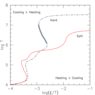
Figure 3: The stability curves for photoionised gas with Solar abundance, $n_{H}=10^{10}\,\,\rm{cm^{-3}}$ and $N_{H}=10^{23}\,\,\rm{cm^{-2}}$ being illuminated by the Soft and the Hard SEDs. A part of the Hard stability curve is highlighted in thick gray - this is the negative slope part of the curve and corresponds to unstable thermodynamic equilibrium. Gas with $\log\xi$ in this part of the curve is unlikely to exist in nature. The Soft curve is stable in the relevant part ($\log T\geq 5.5$) Note that both curves have a part with negative slope at $\log T\lesssim 5.0$. However, this part of the stability curve has such low values of $\log\xi\,\,(<2.0)$ which are not relevant for gas around BHBs.

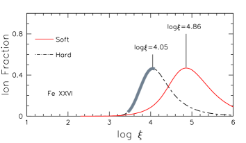
Figure 4: The ion fraction distribution of FeXXVI with respect to $\log\xi$ is shown for the two SEDs, Soft and Hard. The peak of the distribution is marked and the corresponding $\log\xi$ values are labeled. Note that for the Hard SED, a part of the distribution is highlighted by thick gray line - corresponds to the thermodynamically unstable range of $\xi$.

The MHD solutions can be used to predict the presence of outflowing material over a wide range of distances. For any given solution, this outflowing material spans large ranges in physical parameters like ionization parameter, density, column density, velocity and timescales. Only part of this outflow will be detectable through absorption lines - we refer to this part as the “detectable wind”.

Ionization parameter is one of the key physical parameters in determining which region of the outflow can form a wind. There are several forms of ionization parameter in the literature. In this paper we use the definition, more commonly used by X-ray high resolution spectroscopists, namely $\xi=L_{ion}/(n_{H}R^{2}_{sph})$ (Tarter et al. 1969), where $L_{ion}$ is the luminosity of the ionizing light in the energy range 1 - 1000 Rydberg (1 Rydberg = 13.6 eV) and $n_{H}$ is the density of the gas located at a distance of $R_{sph}$. We assume that at any given point within the flow, the gas is getting illuminated by light from a central point source. This simplified approach is not a problem unless the wind is located at distances very close to the black hole ($\leq 100r_{g}$). The SEDs for this radiation has been discussed in the previous Section 3.1.

For detecting the presence of ionized gas, we need to evaluate if the ionization parameter of the gas is thermodynamically stable. Any stable photoionised gas will lie on the thermal equilibrium curve or ‘stability’ curve of $\log T$ vs $\log(\xi/T)$ (Figure 3). This curve is often used to understand the structure of absorbing gas in AGN (Chakravorty et al. 2008, 2009, 2012, and references therein) and BHBs (Chakravorty et al. 2013; Higginbottom & Proga 2015). If the gas is located (in the $\xi-T$ space) on a part of the curve with negative slope then the system is considered thermodynamically unstable because any perturbation (in temperature and pressure) would lead to runaway heating or cooling. Gas lying on the part of the curve with positive slope, on the other hand, is thermodynamically stable to perturbations and hence likely to be detected when they will cause absorption lines in the spectrum.

With version C08.00 of CLOUDY(Ferland et al. 1998). we generated stability curves using both the Soft and the Hard SEDs as the ionizing continuum. For the simulation of these curves we assumed the gas to have solar metallicity, $n_{H}=10^{10}\,\,\rm{cm^{-3}}$ and $N_{H}=10^{23}\,\,\rm{cm^{-2}}$. Assuming these representative average values of $n_{H}$ and $N_{H}$ are reasonable because the stability curves remain invariant when these two parameters are varied over a wide range spanning several decades (see Chakravorty et al. 2013, for details). The Soft stability curve (solid red line in Figure 3) has no unstable region, whereas the Hard one (dotted-and-dashed black line) has a distinct region of thermodynamic instability which is marked by the thick grey line. This part of the curve corresponds to $3.4<\log\xi<4.1$. Thus, this range of ionization parameter has to be considered undetectable, when we are using the Hard SED as the source of ionising light.

Literature survey shows that it is usually absorption lines from H- and He-like Fe ions that are detected (e.g Lee et al. 2002, Neilsen & Lee 2009, Miller et al. 2004, Miller et al. 2006, King et al. 2012). In fact, it is the absorption line from FeXXVI that is most commonly cited as observed. A very important compilation of detected winds in BHBs was presented in (Ponti et al. 2012), and this paper also, concentrates the discussion around the line from FeXXVI. Hence we choose the presence of the ion FeXXVI as a proxy for detectable winds. The probability of presence of a ion is measured by its ion fraction. The ion fraction $I(X^{+i})$ of the $X^{+i}$ ion is the fraction of the total number of atoms of the element $X$ which are in the $i^{\rm{th}}$ state of ionization. Thus,

$$I(X^{+i})=\frac{N(X^{+i})}{f(X)\,N_{\rm{H}}},$$

where $N(X^{+i})$ is the column density of the $X^{+i}$ ion and $f(X)=n(X)/n_{\rm{H}}$ is the ratio of the number density of the element $X$ to that of hydrogen. Figure 4 shows the ion fraction of FeXXVI calculated using CLOUDY. The ion fractions are of course, different based on whether the Soft or the Hard SED has been used as the source of ionization for the absorbing gas. The value of $\log\xi$, where the presence of FeXXVI is maximised, changes from 4.05 for the Hard state, by $\sim$ 0.8 dex, to 4.86 for the Soft state.

In the light of all the above mentioned observational constraints, we will impose the following physical constraints on the MHD outflows (in Sections 4 and 5) to locate the detectable wind region within them:

• In order to be defined as an outflow, the material needs to have positive velocity along the vertical axis ($z_{cyl}$).

• Over-ionized gas cannot cause any absorption and hence cannot be detected. Thus to be observable via FeXXVI absorption lines we constrain the material to have an upper limit for its ionization parameter. We imposed that $\xi\leq 10^{4.86}\,\,{\rm{erg\,cm}}$ (peak of FeXXVI ion fraction) for the Soft state. The ion fraction of FeXXVI peaks at $\xi=10^{4.05}$ for the Hard state, but this value is within the thermodynamically unstable range. Hence for the Hard state, the constraint is $\xi\leq 10^{3.4}\,\,{\rm{erg\,cm}}$, the value below which the thermal equilibrium curve is stable.

• The wind cannot be Compton thick and hence we impose that the integrated column density along the line of sight satisfies $N_{H}<10^{24}{\rm{cm^{-2}}}$.

3.3 Finding the detectable wind within the MHD outflow

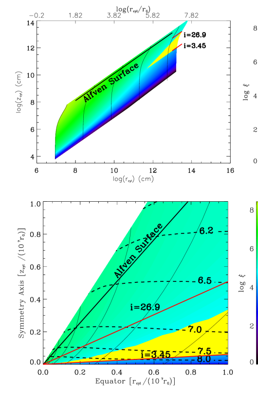
Figure 5: Top Panel: The distribution of the ‘Best Cold Set’ in the logarithmic plane of the radial ($r_{cyl}$) and vertical ($z_{cyl}$) distance (in cylindrical co-ordinates) from the black hole. The distances are also expressed in terms of the gravitational radius $r_{g}$ (top axis), which is $1.5\times 10^{6}\rm{cm}$ for a $10M_{\odot}$ black hole. The colour gradient informs about the $\xi$ distribution of the flow. The solid black lines threading through the distribution show some of the magnetic field lines along which material is outflowing. The Alfvén surface corresponding to the solution is also marked and labelled. The yellow wedge highlights the wind part of the flow - this material is optically thin with $N_{H}<10^{24}\rm{cm^{-3}}$ and has sufficiently low ionization parameter (with $\xi<10^{4.86}\rm{erg\,cm}$) to cause FeXXVI absorption lines. The angular extent of the wind is also clearly marked, where $i$ is the equatorial angle. Bottom Panel: A close up view of the wind region. The distances are expressed in linear scale, but normalised to $10^{7}r_{g}$. The dashed lines show the iso-contours of $n_{H}$, while the associated labels denote the value of $\log n_{H}(\rm{cm^{-3}})$.

In this subsection we demonstrate how we choose the part of the MHD outflow which will be detectable through absorption lines of FeXXVI. For the demonstration we use the MHD solution with $\varepsilon=0.001$ and $p=0.04$ which is illuminated by the Soft SED. Hereafter we will refer to this set of parameters as the “Best Cold Set”. For the purpose of discussion in this subsection, we will work with the Soft SED only, but in subsequent sections additional calculations will be carried out for the scenario where the MHD outflow is illuminated by the Hard SED.

The Best Cold MHD solution provides us with the knowledge of the density of the material at each point within the outflow. Further, we know the Soft SED (both shape and intensity). Hence at each point in the outflow we can calculate the ionization parameter $\xi=L_{ion}/(n_{H}R^{2}_{sph})$. Figure 5 shows the ionization parameter distribution (colour gradient) and the density distribution (iso-density contours on the lower panel) of the outflow due to the “Best Cold Set”. The solid black lines threading through the distribution shows the magnetic field lines along which material is outflowing. The MHD solutions are mathematically self-similar in nature, which essentially means that we can propagate the solutions infinitely. However we have restricted the last streamline to be anchored at $r_{o}=10^{7}r_{g}$. The top panel of the figure is a global view, which shows the entire span of the MHD solution that has been evaluated.

To find the wind region (detectable through FeXXVI absorption lines) within this outflow we have to impose the three required physical conditions listed in Section 3.2. The resultant wind region is highlighted as the yellow wedge in Figure 5. We see that the wind is detected only from the outer parts of the flow with $\log R_{sph}|_{\rm{wind}}/r_{g}\geq 5.4$. The lowest and highest equatorial angle ($i$) of the line of sight are clearly marked for the wind region (in both panels). The observer will have to view the BHB within this angular range to be able to detect the wind. The wind is equatorial, for the ‘Best Cold Set’, not extending beyond $i=26.9^{\circ}$. In the lower panel of Figure 5 we use a linear (but normalised by $10^{7}r_{g}$) scale for $r_{cyl}$ and $z_{cyl}$, which renders us a close up view of the wind region within the solution. The labelled dashed black lines are the iso-contours for the number density $\log n_{H}(\rm{cm^{-3}})$. The velocities $v_{obs}$ (not shown in the Figure) in this region fall within the range $10^{2}-10^{3}\rm{km\,s^{-1}}$.

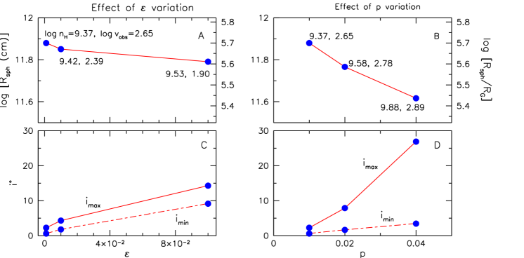
Figure 6: The physical parameters of the wind are plotted as a function of $\varepsilon$ (left panels) and $p$ (right panels), while using the Soft SED as the ionizing continua. Top Panels: For the closest wind point, we plot the logarithm of $R_{sph}|_{wind}$ in the left panel A as a function of the disk aspect ratio $\varepsilon$ and as a function of the accretion index $p$ in the right panel B. $p=0.01$ is held constant for the solutions in the left panels and $\varepsilon=0.001$ is kept constant for those in the right panels. Each blue circle in the figure represents a MHD solution. The logarithm of two other relevant quantities, $n_{H}$ and $v_{obs}$ for the closest wind point are labeled at each point - these are their maximum possible values within the wind region, for a given MHD solution. Bottom Panels: The minimum ($i_{min}$) and the maximum ($i_{max}$) equatorial angles of the line of sight, within which the wind can be observed, is plotted as a function of $\varepsilon$ (left) and of $p$ (right).

This same method of finding the wind, and the associated physical conditions is used for all the cold MHD solutions considered in this paper. In the subsequent sections we will vary the MHD solutions (i.e. $\varepsilon$ and $p$) and investigate the results using both the Soft and Hard SEDs.

To ensure that the wind is in thermal equilibrium, it is important to compare the various physical timescales. We used CLOUDY to evaluate the cooling time scales at each point within the wind region of the solution. CLOUDY assumes that atomic processes (including photoionization and recombination cooling) occur on timescales that are much faster than other changes in the system, so that atomic rates have had time to become “time-steady”. These atomic processes, in addition to some other continuum processes like Comptonization and Bremsstrahlung, are responsible for heating and cooling the gas. Whether the atomic processes dominate over the continuum processes is determined by the ionization state and/or the temperature of the gas. For photoionized wind we expect the atomic processes to dominate. However, one way to make sure that the gas satisfies the time-steady condition (which is assumed by CLOUDY) is to check the CLOUDY computed cooling time scale against the dynamical time scales from our physical MHD models. CLOUDY defines the cooling time scale as the time needed to loose half of the heat generated in the gas due to various atomic and continuum processes. Thus thermal equilibrium is also ensured as long as the cooling time scale is smaller than the dynamical time scale $\tau_{dyn}$ - which was found to be true within the wind region of the outflow for the ‘Best Cold Set’.

4 The cold MHD solutions

4.1 Effect of variation of the parameters of the MHD flow

Here we aim to find which of the two parameters $\varepsilon$ and $p$ is more influential in producing the wind. The value of $p$ and $\varepsilon$ decides the density of material at the launching point of our magneto-hydrodynamic outflow (Equation 2). The extent of magnetisation in the outflow is also dependant on $p$ (Section 2). It is these two parameters that links the density and other physical properties of the outflow with the accretion disk. Since a particular pair of $p$ and $\varepsilon$ will result in a unique MHD solution, we can generate different MHD solutions, by changing the values of $p$ and $\varepsilon$. On each of these solutions, we perform the methods described in the previous Section 3.3 and investigate the wind part of the outflow.

To judge the influence of $p$ and $\varepsilon$, in a quantitative way, we compare some physically relevant parameters of the wind. For observers, one important set of wind parameters are the distance, density and velocity of the point of the wind closest to the black hole. Hereafter we shall call this point as the ‘closest wind point’. Another quantity of interest would be the predicted minimum and maximum angles (of the line of sight) within which the wind can be observed. We conduct this exercise using both the SEDs - Soft and Hard. The results are plotted in Figure 6.

The exact value of these quantities should not be considered very rigorously, because the value is decided by the various constraints that we have applied. It is more important to note the changes in these quantities as $\varepsilon$ and $p$ vary. The relative changes should be used to assess how variations in $\varepsilon$ and $p$ increase the possibilities of detecting the wind.

4.1.1 Variation of the disk aspect ratio $\varepsilon$

For the closest wind point, we plot $R_{sph}|_{wind}$ versus the value of $\varepsilon$ of the MHD solution, in panel A of Figure 6. Further, $n_{H}$ and $v_{obs}$ for this point are labelled. Using the Soft SED, the closest wind point reaches closer to the black hole by a factor of 1.06 as $\varepsilon$ increases from 0.001 to 0.01, and then by a farther factor of 1.14 as $\varepsilon$ increases to 0.1. The density at the closest point is $n_{H}|_{max}=10^{9.37}\rm{cm^{-3}}$, for $\varepsilon=0.001$ . Note that for any given solution, the density at the closest point is the maximum attainable density within the wind region, for that particular MHD solution. This maximum attainable density of the wind, increases as $\varepsilon$ increases to 0.01 and then to 0.1. However, as a function of $\varepsilon$, the variation in this quantity is not very high, but only 0.16 dex. Like density, for a given solution, the velocity at the closest wind point, $v_{obs}|_{max}$, is the highest that can be attained by the detectable wind. This quantity monotonically decreases by 0.26 dex and then by 0.49 dex as $\varepsilon$ increases from 0.001 to 0.01 and then to 0.1. This means, to get winds with higher speed, we need disks with higher aspect ratios.

$i_{min}$ is the minimum and $i_{max}$ the maximum equatorial angles of the line of sight, within which the wind can be detected. Panel C of Figure 6 shows the changes in the angles as $\varepsilon$ varies. One can easily judge the angular extent of the wind by gauging the difference between $i_{min}$ and the maximum angles, for a particular solution (and SED). $i_{min}$ rises from 0.60 to 1.78 to 9.15 and $i_{max|{Soft}}$ increases from 2.27 to 4.31 to 14.3 as $\varepsilon$ varies from 0.001 to 0.01 to 0.1. The growth of $\Delta i=i_{max}-i_{min}$ with $\varepsilon$ shows that the wind gets broader as the disk aspect ratio increases.

4.1.2 Variation of the ejection index $p$

As $p$ increases, the wind moves closer to the black hole (panel B of Figure 6) - $R_{sph}|_{wind}$ drops by a factor of 1.3 as $p$ goes from 0.01 to 0.02 and then reduces further by a factor of 1.41 when $p$ is increased to 0.04, while using the Soft SED. The total change in the density of the closest wind point is 0.51 dex as $p$ changes from 0.01 to 0.04. Thus both $R_{sph}|_{wind}$ and $n_{H}|_{max}$ are effected more by the variation in $p$ than by the variation in $\varepsilon$ (within the range of these parameters investigated by us). The velocity $v_{obs}|_{max}$ of the closest point however, varies far less with change in $p$, the total decrease being only 0.24 dex.

$i_{min}$ and $i_{max}$ as a function of $p$ (using the Soft SED) is shown in panel D of Figure 6. As $p$ goes from 0.01 through 0.02 to 0.04, the minimum angle rises from 0.60 through 1.65 to 3.45, a range rather smaller than that caused by the $\varepsilon$ variation. $i_{max}$ goes from 2.27 to 7.89 to 26.9. Thus the growth of $\Delta i$ is rendered to be higher as a function of increase in $p$, implying a higher probability of detecting a wind when the flow corresponds to higher $p$ values. Since $p$ is the relatively more dominant (compared to $\varepsilon$) disk parameter in increasing the density at a given distance, the resultant outflowing material has lower ionisation. This is a favourable influence to cause detectable winds.

4.2 Cold solutions for the Hard state

For the entire range of $\varepsilon$ (0.001 - 0.1) and $p$ (0.01 - 0.04) we analysed the MHD solutions illuminated by the Hard SED, as well. Note that for the Hard SED, we have to modify the upper limit of $\xi$ according to the atomic physics and thermodynamic instability considerations (Section 3.2). With the appropriate condition, $\log\xi\leq 3.4$, we could not find any wind portions within the Compton thin part of the outflow, for any of the MHD solutions.

This is a very significant result, because this provides strong support to the observations that BHBs do not have winds in the Hard state. We will discuss this issue further complimented with better quantitative details in Section 6.3.

4.3 The need for Warm MHD solutions

The density reported for most of the observed BHB winds $\geq 10^{11}\,\rm{cm^{-3}}$ and the distance estimates place the winds at $\leq 10^{10}\,\rm{cm}$ (Schulz & Brandt 2002; Ueda et al. 2004; Kubota et al. 2007; Miller et al. 2008; Kallman et al. 2009). Our analysis in the previous subsections show that $R_{sph}|_{wind}$ is too high and $n_{H}|_{max}$ is too low even for the ‘Best Cold Solution’ to match observations. The purpose of this section is to understand which parameter of the accretion-ejection process can provide us with a MHD solution capable of explaining observed (or derived) parameters of BHB winds. Studying the effect of the disk parameters gives us a clear indication that increasing the value of the ejection index $p$ favours the probability of detecting winds, as demonstrated by the larger extent of increase in $\Delta i$. Further, the increase in $p$ results in two more favourable effects - the closest wind point moves closer to the black hole and causes a higher increase in density.

The above phenomenological tests of the $\varepsilon-p$ space, indicates that a MHD solutions with higher $\varepsilon$, say 0.01, and a high $p\geq 0.04$ would be the better suited to produce detectable winds, comparable to observations. However there are limitations on the $\varepsilon-p$ combination imposed by the physics of the MHD solutions (see Figure 1) and it is not possible to reach larger values of $p$ for the cold solutions with isothermal magnetic surfaces. As shown in Casse & Ferreira (2000b), to get denser outflows with larger $p$, some additional heating needs to take place at the disk upper layers leading to a warming up of the wind. The authors argued that the origin of this extra heating could be due to illumination from an external source or enhanced turbulent dissipation within the disk surface layers. Let us now investigate in the following section if a warm solution is indeed, much better for producing winds matching observations.

5 Warm MHD solutions

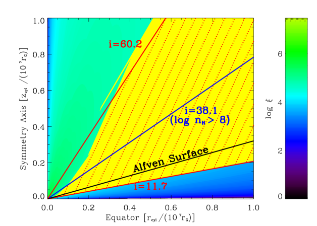
Figure 7: The ionization parameter distribution for a Warm MHD solution with $\varepsilon=0.01$ and $p=0.10$. The yellow region within the outflow is obtained in the same way as in Figure 5. The shaded region (with dotted red lines) is the wind region within such a warm outflow - to obtain this region we used the additional constraint that the cooling timescale of the gas has to be lower than the dynamical time scale. Further, the solid blue line with $i=38.1^{\circ}$ is drawn to depict that high density material ($\log n_{H}\geq 8.0$) in the flow is confined to low equatorial angles.

In this section we investigate the properties of the wind as a function of increasing $p$, but for warm MHD solutions. Here we choose to ignore the effect of $\varepsilon$, because in the previous section we found that variation in $\varepsilon$ (over two orders of magnitude) has very little effect on changing the physical quantities of the wind. Further, in the previous sections we found that the wind does not exist for the Hard SED. Hence, we shall conduct the extensive calculations with the Soft SED only. We shall however, discuss winds in the Hard state in Section 6.3 as a part of general discussions.

Self-confined outflows require $\sigma^{+}\simeq 1/p$ larger than unity, as pointed out through Equation 4 in Section 2.2. Moreover, the power in the outflow is always a sizable fraction of the mechanical power

$$L_{acc}=\left[\frac{GM_{BH}\dot{M}_{acc}(r)}{2r}\right]^{r_{in}}_{r_{out}}$$ (12)

released by the accreting material between the inner radius $r_{in}$ and the outer radius $r_{out}$. Because $\dot{M}_{acc}(r)\propto r^{p}$ in a disk, launching outflows, one gets $L_{acc}=0$ for $p=1$. This is why, unless there is an external source of energy, $p=1$ is a maximum limit, and in fact, powerful magnetically driven flows require a much smaller ejection index. To consider what highest value of $p$ should be aimed for, we scout the literature. We find two relevant references, namely,
(a) Casse & Ferreira (2000b) who computed warm MHD accretion-ejection solutions up to $p=0.456$ to model winds mostly, in young stellar objects and
(b) a series of papers by Fukumura et al. (Fukumura et al. 2010a, b, 2014, 2015), who used a model with $p=0.5$.
Hence while attempting to generate the disk surface heated, magnetically driven and magnetically confined outflows, we will limit ourselves to $p\leq 0.5$.

For this paper, we obtain dense warm solutions (with higher values of $p$, i.e. $p\geq 0.04$) through the use of an ad-hoc heating function acting along the flow. This additional heating needs to start within the disk itself, in the resistive MHD layers, in order to cause a larger mass loading at the base of the outflow. However, the heating requires to be maintained for some distance within the outflow too, into the ideal MHD zone. This is necessary in order to help the launching of these dense outflows and tap the thermal energy content instead of the magnetic one (refer to Casse & Ferreira 2000b, for more details). It must therefore be realized that any given “warm solution” from a near Keplerian accretion disk is based on an ad-hoc heating term (the function $Q$ in Casse & Ferreira 2000b, , see also Section A of Appendix). The physical mechanism behind the heating term has not been specified. However, a posteriori calcualtions show that even a few percents of the released accretion energy would be enough to give rise to such warm MHD winds. Whether or not MHD turbulence in accretion disks can provide such a surface heating is an open theoretical issue. For further discussion on this see Section A of the Appendix. On the other hand the heating could be caused by the illumination form the interior parts of the disk. To determine and/or distinguish between the physical cause of the heating is a rigorous theoretical study in itself and is beyond the scope of this paper.

To ease comparison between various warm models, we use the same shape for the heating function, while playing only with its normalization to increase $p$ (the larger the heat input, the larger the value of $p$, see Figure 2 in Casse & Ferreira 2000b). For $\varepsilon=0.01$ we could achieve a maximum value of $p=0.11$. For the purpose of this paper, it is not required to provide the “most massive” (i.e. largest possible $p=0.5$) solution - it is enough to show general trends. However, we are developing the methods to generate denser MHD solutions with $p=0.5$ and these solution(s) will be reported in our subsequent publications where we will attempt to model the winds observed in specific outbursts of specific BHBs.

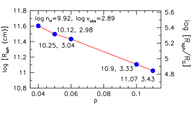
Figure 8: Distance (density and velocity) of the closest wind point is (are) plotted (labelled) as a function of $p$ for all the warm MHD solutions that we investigated. $\varepsilon=0.01$ is constant.

Figure 7 shows the wind for a Warm MHD solution with a rather high $p=0.10$. The wind (yellow region) spans a much wider range (than even the “Best Cold Solution”) and extends far beyond the Alfven surface which was not the case for the cold MHD solutions. Hence we introduce an additional constraint derived from timescale considerations. The lower angular limit ($i=11.7^{\circ}$) is derived due to the constraints of $\xi$ and $N_{H}$. Next, we used CLOUDY to calculate the cooling timescales of the gas at each point within the yellow wind region of the outflow. Note that for the timescale calculations using CLOUDY (which are computationally expensive) we have used a much coarser grid of $i$ than that used for other calculations of the MHD solutions. This is sufficient for our purpose here, where a coarse upper limit on $i$ is sufficient. To be consistent with a photoionised wind which is in thermal equilibrium, the cooling timescale needs to be shorter than the dynamical timescale. This timescale condition was satisfied within the yellow region if $i\leq 60^{\circ}$. Thus the red-dotted shaded region is the resultant detectable wind. However, note that the densest parts of the wind is confined to low equatorial angles. For example, gas with $n_{H}\geq 10^{8}\,\rm{cm^{-3}}$ will lie below $i=38.1^{\circ}$. For this solution, we further calculated $B_{z}\sim 70$ Gauss (Equation 6) at the disk mid plane at a distance $r_{cyl}=R_{sph}=1.28\times 10^{11}\rm{cm}$.

We investigated warm MHD solutions with a range of values of $p$. In Figure 8 we have plotted the distance of the closest wind point for all those solutions. Each point is also labelled with the respective values of density and velocity. Between the $p=0.04$ solution and the one with the highest $p=0.11$ (that we could achieve) $R_{sph}|_{wind}$ goes closer by a factor of 3.79 and stands at $7.05\times 10^{4}\,r_{g}$. The highest density that we could achieve is $\log n_{H}=11.1$ and the highest velocity is $\log v_{obs}=3.43$. Hereafter we shall refer to the $\varepsilon=0.01$ and $p=0.10$ warm MHD solution as the “Best Warm Solution”.

Clearly, warm solutions do a much better job than cold ones, as expected. However, some observational results require the winds to have higher density and lower distance than those produced by the “Best Warm Solution”. In the following section we discuss the possibilities in which we can theoretically achieve more stringent values demanded by observations of some extreme winds.

6 Discussions

6.1 Towards the extreme MHD winds

6.1.1 Choice of upper limit of $\xi$

The ionization parameter is the key parameter in defining the wind region within the outflow. Here we discuss (a) the possibility of changing $\xi$ if $\dot{m}$ changes and (b) the effect if the upper limit of $\xi$ is changed.

(a) In the definition of $\xi$, the density $n_{H}$ in the denominator is proportional to $\dot{m}$ (see Equation 5). In the numerator, $L_{ion}\propto L_{rad}$ and we also assume $L_{rad}$ to be proportional to $\dot{m}$ (see Section 3.1). Hence for a given MHD solution, changing $\dot{m}$ will not change the $\xi$ distribution within the outflow.

In the case of inefficient accretion flow like ADAF, $L_{rad}\propto\dot{m}^{2}$, and changes in $\dot{m}$ could have some effects. However, we are considering here, physical scenarios, where the accretion disk is radiatively efficient with $\dot{m}_{obs}\sim 0.1$. Hence, accepting $L_{rad}\propto\dot{m}$ is a reasonable assumption.

(b) We used the limit $\log\xi\leq 4.86$ to define the detectable wind. Note that for the Soft SED, $\log\xi=4.86$ corresponds to the peak of the ion fraction of FeXXVI (Figure 4). The ion can have significant presence at higher $\xi$. For example, at $\log\xi=6.0$ FeXXVI is still present, but at $\sim 1/4$ of its peak value. Further, there are other ions (including NiXXVIII) which peak at higher values of $\xi$ (see Figure 4 of Chakravorty et al. 2013). Such ions have been reported in Miller et al. (2008). In fact such ions may be routinely detected in data from the future X-ray telescopes like Astro-H and Athena. It is thus instructive to investigate how the properties of the closest wind point (for a given solution) are modified when the constraint on upper limit of $\log\xi$ are changed.

For the best warm solution we calculated the physical parameters for the closest wind point with a modified upper limit $\log\xi=6.0$. We find that $R_{sph}|_{wind}$ decreases by a factor of 93.4 bringing this point to $9.1\times 10^{2}r_{g}$. The density at this point is $\log n_{H}=13.71$ and the velocity is $\log v_{obs}=4.28$. Thus we see that the parameters of closest point is sensitively dependant on the choice of the upper limit of $\xi$.

6.1.2 The need for denser warm solution

From the analysis presented in Section 4.1 and Section 5 it is clear that MHD solutions with larger $p$ favour winds which are closer to the black hole. Even for the densest solution discussed in this paper, with $\varepsilon=0.01$ and $p=0.11$, we cannot predict a wind closer than $7.05\times 10^{4}\,r_{g}$ (for $\log\xi\leq 4.86$) and denser than $\log n_{H}>11.07$ . However Miller et al. (2008) discussed that the wind in GRO J1655-40 was very dense, where $\log n_{H}\geq 12$, and hence had to be very close to the black hole at $\sim 10^{3}r_{g}$. Thus, to explain such extreme winds, we need denser warm MHD solutions with higher $p$.

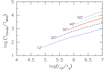
Figure 9: Comparison of the different temperatures associated with wind in the Best Cold Solution. $T_{Cloudy}$ is the temperature calculated using CLOUDY and is the actual temperature of the photoionized gas. $T_{MHD}$ is the temperature du to the MHD solution - the value that has been used to calculate all the physical properties of the outflow. The ratio between these two temperatures are plotted as a function of the distance from the black hole and at different angles of line of sight.

In the context of AGN, Fukumura et al. (2010a, b, 2014, 2015) have been able to reproduce the various components of the absorbing gas using MHD outflows which would correspond to $p\simeq 0.5$. As discussed in Section 5, we have not been able to reproduce such high values of $p$ and are limited to $p=0.11$. Our calculations in the previous section shows that as $p$ increased from 0.04 to 0.11 for the warm MHD solution, $R_{sph}|_{wind}$ for the closest wind point decreased by a factor of 3.79. Thus a further increase to $p\simeq 0.5$ may take the closest wind point nearer to the black hole by a further factor of $\sim 10$ to $\sim 5\times 10^{3}r_{g}$. The above hypothetical numbers are assuming an almost linear change in density as $p$ increases. In reality, the progression of the physical quantities in the denser MHD solutions may not be that simple. We shall report the exact calculations in our future publications.

As our analyses stand now, even with denser warm MHD solutions with $p=0.5$ we do not expect the wind to exist closer than $\sim 5\times 10^{3}r_{g}$, if $\log\xi<4.86$. However, note from the discussion in the previous subsection, this distance may be reduced by a factor of $\sim 90$ to few $<10^{2}r_{g}$ for a modified constraint of $\log\xi<6.0$. The density and velocity will be increased accordingly. These speculative numbers indicate that indeed the warm MHD outflow models may be able to explain even the most extreme winds observed (Miller et al. 2008; King et al. 2012; Diaz Trigo et al. 2013). The aforementioned speculations strongly indicate to us the kind of MHD solutions that we need to generate to fit observations. However a confirmation of this speculations is beyond the scope of this paper. We will report the exact calculations for the extreme MHD models in our subsequent papers.

6.2 Temperature of the outflowing gas

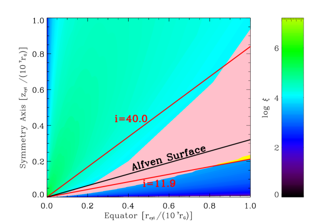
Figure 10: The wind characteristics, when the “Best Warm Solution” is illuminated with a Hard SED. The drastically reduced (compared to Figure 7) yellow region within the outflow is obtained in the same way as in Figures 5 and 7. We can only see a very small portion of this yellow region at $r_{cyl}/(10^{7}r_{g})>0.8$. The rest of this yellow region is occulted by the pink wedge which represents the part of the outflow which is thermodynamically unstable and has $3.4\leq\log\xi\leq 4.05$. Note that a small part of this unstable outflow is within the Compton thick region with $\log N_{H}>24$ (portions below the line marking the low angle $i=11.9^{\circ}$).

The physical properties of the MHD solutions depend on the energy equation which involves solving the balance between the local heating and cooling effects. Hence, along with all the other properties, like the velocity, density etc. the temperature ($T_{MHD}$) of the outflowing gas is also specified - see discussion in Section A of the Appendix. However, the MHD calculations do not take into account the effect of photoionization of the outflowing material due to light from the central source. In fact, the temperature of the gas within the wind region is determined by the effects of photoionization by the ionizing SED and may be very different from $T_{MHD}$.

We used CLOUDY to calculate the temperature $T_{Cloudy}$ of the gas to check how different it is from $T_{MHD}$ for the best warm solution and the comparison is shown in Figure 9. CLOUDY calculations are computationally expensive and hence we restricted them to within the wind region (the shaded region with dotted red lines) of the outflow only. Note that for the best warm solution, below $i=11.7^{\circ}$ the gas is Compton thick with integrated $N_{H}>10^{24}cm^{-2}$. Hence photoionization and associated acceleration of the Compton thick gas may be negligible. As such, the properties of the outflow in the Compton thick region of the outflow is likely to be determined by magnetic fields alone. To determine whether this qualitative assumption is true is beyond the scope of the paper (although, see Section 3.4 of Garcia et al. 2001 for detailed methodology of how one might attempt to solve the energy equation along a flow field line involving both the MHD dynamical terms and a photoionization code). Hence we compare temperatures within the Compton thin wind region only.

Figure 9 shows that $T_{Cloudy}$ is indeed different from $T_{MHD}$ and the difference increases as we move away from the surface of the accretion disk and as we move further out. We need to judge at this point, if this difference in the gas temperature, and hence on its enthalpy, will make a difference to the properties of the gas.

Figures 13 and 14 of the Appendix show that the specific enthalpy term is negligible compared to the specific magnetic energy. Comparing the specific energies, we see that even if the gas temperatures were higher (due to photoionization) than $T_{MHD}$ by orders of magnitude, the magnetic field would still dominate the specific energy and hence the properties of the outflow would still be determined by the magnetic field.

6.3 Effect of thermodynamic instability in the Hard state

Conventionally it is assumed that ionized gas cannot be detected if it is thermodynamically unstable. Chakravorty et al. (2013) showed the effect of thermodynamic considerations and found that the equilibrium curve to be unstable for a range of $\xi$ values, but only for the Hard SED. We have conducted stability curve analysis in Section 3.2 and have found similar results - for the Hard SED, the range $3.4<\log\xi<4.1$ is thermodynamically unstable. Thus the constraints on $\xi$ have to be modified accordingly, when looking for the wind region within an outflow illuminated by the Hard SED.

In Section 4.2 we have mentioned that with the appropriate restrictions on the $\xi$ value, no wind could be found within the cold MHD outflows. Since the warm solutions result in much broader (than that in cold solutions) wind region, we test if the best warm solution can have a wind with a Hard SED.

Using the value $\log\xi=4.05$, we get a significant (although reduced from the Soft SED case) wind region. Next, we check the effect of thermodynamic instability. In Figure 10 the pink region shows the part of the outflow which has $\log\xi=3.4-4.05$, a range that is “thermodynamically unstable”. Note that above the $i=11.9^{\circ}$ line (which marks the Compton thick limit), this thermodynamically unstable zone almost completely occults the wind region (in yellow). This implies that in the Hard state, even if a significant region of the outflow is Compton thin and has the correct $\log\xi$ to produce FeXXVI lines, this same region is also thermodynamically unstable. Hence in the Hard state, we cannot expect to detect the wind.

Our analysis thus, strongly suggests that winds will not be detected in the Hard state. Hence, we are in agreement with observational results which detect winds only in the Softer states of the outburst (Ponti et al. 2012). Note that such a correlation between accretion state (Softer) and presence of wind has been found for neutron stars as well by Ponti et al. (2014). Thus our analysis and results maybe valid, not only for BHBs but neutron star accretion disks as well.

We would want to discuss, at this point, an interesting observation made by Higginbottom & Proga (2015) on the issue of thermodynamic instability. The authors correctly point out that, if a parcel of gas reaches a thermodynamically unstable temperature (where the gradient of the stability curve becomes negative - see Figure 3) the gas will quickly heat up to attain the higher temperature of the next thermodynamically stable point at same pressure (same $\xi/T$). For a thermally driven wind this effect would result in very efficient acceleration. However for a MHD wind this effect, particularly relevant for the Hard State, will not aid in the wind driving mechanism. In the Hard state (from Figure 3) the maximum increase of temperature, for a parcel of gas to avoid thermodynamic instability, is about an order of magnitude. In the previous subsection we have demonstrated that $T_{Cloudy}$ could be much higher than $T_{MHD}$ and still not affect the properties of the MHD driven wind. For a typical angle of $i=20^{\circ}$, (see Figures 9 and 14), even if $T_{Cloudy}$ were higher by an order of magnitude (raised by thermodynamic instability considerations), the magnetic specific energy would still dominate over that of enthalpy. Hence, for MHD winds, thermodynamic instability is unlikely to cause any additional efficient acceleration. We acknowledge that thermal lifting might play a role in the disk upper layers, where the disk material gets magneto-centrifugally accelerated. But it is unclear whether or not photoionisation equilibrium would correctly describe these highly expanding layers.

7 Conclusions

Winds are detected as absorption lines in the high resolution X-ray spectra of black hole binaries. The absorption lines are mostly from H-like and He-like Fe, but some rare observations show lines from other ions. Ponti et al. (2012) have shown that winds are seen in the Soft state of the outburst and never in the canonical Hard states. Further, the strongest winds were observed for objects with high inclination angles, i.e. the winds flow close to the disk surface at low equatorial angles. In this paper we investigated if magneto centrifugal outflows (Ferreira 1997; Casse & Ferreira 2000b) can reproduce the observed winds in terms of the correct range of ionization parameter ($\xi$), column density ($N_{H}$), velocity ($v_{obs}$) and density $n_{H}$. The investigations are done as a function of the two key accretion disk parameters - the disk aspect ratio $\varepsilon$ and the radial exponent $p$ of the accretion rate ($\dot{M}_{acc}\propto r^{p}$). We further test if our theoretical models can match the state dependant and angle dependant nature of the accretion disk winds. The results of our study are listed below:

1. The cold solutions, which are solely driven by the magnetic acceleration, produce very narrow regions of detectable wind and from the outer parts ($\geq 2.51\times 10^{5}r_{g}$) of the accretion disk. In addition, the cold MHD winds have lower density ($\log n_{H}\leq 9.9$) than what observations predict. The winds were found to be equatorial, within $i\sim 30^{\circ}$ of the accretion disk surface.

2. We realised that we need high values of $p(>0.04)$ to reproduce winds that can match observations. However $p$ cannot be increased to desirable values in the framework of the cold MHD solutions. We definitely need warm MHD solutions to explain the observational results. In the warm MHD solutions, some extra heating at the disk surface causes a larger mass loading at the base of the outflow, which is then magnetically accelerated to form a denser wind. We speculate that the aforementioned heating may be due to the illuminating SED, particularly in the Soft state, or due to dissipation of energy by MHD turbulence, within the disk. Indeed, even a few percents of the released accretion energy (if it were deposited on the disk surface, leading to local heating there, instead of being dissipated deep within the disk layers), would be enough to give rise to such warm MHD winds. Whether or not MHD turbulence in accretion disks provides such a surface heating is an open theoretical issue.

3. In the Soft state, our densest warm MHD solution predicts a wind at $7.05\times 10^{4}r_{g}$ with a density of $\log n_{H}=11.1$. The densest part of the wind ($\log n_{H}>8$) still remains equatorial - within $i\sim 30^{\circ}$ of the accretion disk. The values of the physical parameters are consistent with some of the observed winds in BHBs. However, there are some other extreme observations (e.g of GRO J1655-40 Miller et al. 2008) which require a denser wind which is at a smaller distance to the black hole. From our work we understand what kind of MHD solutions can reproduce such extreme winds - warm MHD solutions with $p\simeq 0.5$. It was beyond the scope of this paper to produce those particular solutions. However, we will generate and report such solutions in our future publications where we will attempt to reproduce spectra of BHB winds of different kinds.

4. The outflow illuminated by a Hard SED will not produce detectable wind because (i) the allowed region of the winds is smaller (compared to the Soft SED case) and (b) the wind region falls within the thermodynamically unstable range of $\log\xi$ and hence unlikely to be detected.

5. Thus in the framework of MHD outflows we can satisfy the observed trends reported in Ponti et al. (2012, and references therein) that - (a) winds are observed in the Soft states (and not expected in the Hard state) of the BHB outbursts and (b) accretion disk winds in BHBs are equatorial. We have been able to reproduce the expected values (consistent with observations) of distance, density and velocity for the average winds in BHBs. For the extremely dense (and hence at small distances from the black hole) winds our rigorous analysis was capable of pointing to the kind of accretion disks which will be able to reproduce them.

Appendix A Cold versus warm disk wind solutions

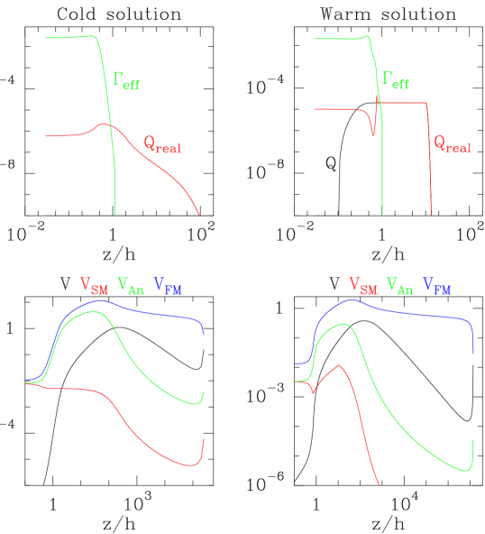
Figure 11: Profiles along a magnetic surface of a typical cold -isothermal- solution with $p=0.006$ (left) and warm solution with $p=0.1$ (right). Top: effective turbulent heating $\Gamma_{eff}$, real entropy generation term $Q_{real}$ and prescribed function $Q$ in arbitrary units. Bottom: critical velocities (see text) normalized to the disk mid plane sound speed.

In this appendix, we highlight some important points allowing to distinguish between ”cold” and ”warm” wind solutions from near-Keplerian accretion disks. In the terminology of Blandford & Payne (1982), a cold wind refers to a flow where the enthalpy is negligible with respect to the magnetic energy density at the base, namely at the disk surface. Unless some additional heating source occurs within the disk layers and/or at its surface, the temperature of the flow leaving the disk is at most comparable to that prevailing at the disk mid plane. This translates into an enthalpy which is roughly $(h/r)^{2}$ times the gravitational potential, hence negligible in a thin disk. As a consequence, a wind with a positive Bernoulli integral can only be achieved by magnetic means. Cold models have been thus computed using different prescriptions for the thermal state of the magnetic surfaces: either isothermal (constant temperature along a surface, eg. Ferreira (1997)) or adiabatic surfaces (decreasing temperature, eg Casse & Ferreira (2000a)).

Figure 12: Shape of the magnetic surfaces (top left) and vertical profiles along the magnetic surfaces of (a) outflow poloidal velocity normalized to the Keplerian speed at the field line anchoring radius $r_{o}$ (top right), (b) density normalized to its mid plane value (bottom left) and (c) temperature normalized to its mid plane value (bottom right). Solid lines are for the warm solution, dashed for the isothermal.

On the contrary, warm disk wind models rely on the existence of some ad-hoc entropy generation term $Q$. The exact energy equation for the outflowing material writes

$$\rho T\frac{dS}{dt}=\rho T\@vec{u_{p}}\cdot\@vec{\nabla}S=Q_{real}$$ (13)

where $S$ is the specific entropy and $Q_{real}$ is the local source of entropy which arises from the difference between all heating and cooling processes (Casse & Ferreira (2000b)). More specifically, it can be written $Q_{real}=(\Gamma_{eff}+\Gamma_{turb}+\Gamma_{ext})-(\Lambda_{rad}+\Lambda_{turb})$, where $\Gamma_{eff}=\eta_{m}J^{2}_{\phi}+\eta^{\prime}_{m}J^{2}_{p}+\eta_{v}r\left|\@vec{\nabla}\Omega\right|^{2}$ is the effective Joule and viscous heating, $\Gamma_{turb}$ is a turbulent heating term that cannot be described by simple anomalous transport coefficients (namely the term $\Gamma_{eff}$) and would correspond, for instance, to some resonant or wave heating above the disk, $\Gamma_{ext}$ is an external source of energy (typically due to some illumination by UV or X-rays, if present at all). $\Lambda_{rad}=\@vec{\nabla}\cdot\@vec{S}_{rad}$ is the radiative cooling ($\@vec{S}_{rad}$ being the radiative flux) and $\Lambda_{turb}$ is a cooling due to a turbulent energy transport, which is most probably also taking place inside turbulent disks (see Casse & Ferreira (2000b) for more details).

Taking into account all these processes is a tremendous task which requires the understanding not only of MHD turbulence in outflow emitting disks, but also of the complex radiative processes at work in various astrophysical objects. A simplified approach is actually to assume the entropy generation term, which is what we do. The above exact energy equation follows the flow streamlines, which is inconvenient to use when integrating the equations from the disk mid plane to outflow asymptotics (isothermal solutions cannot be obtained for instance). Hence, instead, the energy equation actually solved is

$$\frac{\rho u_{p}}{B_{p}}\@vec{B_{p}}\cdot\nabla C_{s}^{2}=(\gamma-1)\left(Q+C_{s}^{2}\frac{\rho u_{p}}{B_{p}}\@vec{B_{p}}\cdot\nabla\ln\rho\right)$$ (14)

where $\gamma$ is the adiabatic index and $C_{s}^{2}=P/\rho$ with a prescribed self-similar function $Q$ described in Section 4.1 of Casse & Ferreira (2000b). This equation is strictly equivalent to Eq.(13) in the ideal MHD outflow region and allows to treat the disk vertical structure. Once a full trans-Alfvénic MHD flow solution is obtained, the real entropy generation term $Q_{real}$ can be computed using Eq.(13) as shown in Figure 11.

To illustrate cold and warm solutions, we choose two representative super-Alfvenic solutions with same $\varepsilon=0.01$. The cold solution is isothermal ($\gamma=1$) with $p=0.006$, whereas the warm solution with $\gamma=5/3$ has $p=0.1$ and requires a heating function $Q$. The upper panels of Figure 11 show, for both solutions, the vertical profiles along a magnetic surface of the effective turbulent heating $\Gamma_{eff}$ and the imposed $Q$, as well as the real $Q_{real}$, entropy generation terms. The entropy parameter, defined as

$$f=\frac{\int_{V}Q_{real}dV}{\int_{disk}\Gamma_{eff}dV}$$ (15)

where the volume $V$ is both the disk and the wind, can be computed a posteriori once a solution is found. It provides the ratio of the power due to the extra heating going into the wind to the turbulent power dissipated within the disk. The warm solution resulted in an entropy parameter f = 0.02, which suggests that local MHD turbulence could actually lead to such solution. Indeed, the required extra heating amounts only to 2% of the power that would be dissipated within the disk (hence a reduction of 2% of the disk luminosity). This would be possible if MHD turbulence itself ($(\Gamma-\Lambda)_{turb}$ terms) conveys that power to the disk upper layers (the ’base of the wind’). This is an open theoretical issue of course. If such a process proves to be inexistent, then one should rely only on illumination ($\Gamma_{ext}$ term) to obtain warm MHD solutions of this kind. Note that magneto-centrifugal winds undergo a huge adiabatic cooling at the disk surface so that to remain isothermal requires some heat deposition as well. Thus, the cold solution displayed here would require a $Q_{real}$ such that $f=1.6\times 10^{-3}$. The lower panels show the profiles of the various velocities relevant in such MHD flows: the critical flow speed $V$, the slow $V_{SM}$ and fast $V_{FM}$ magnetosonic phase speeds and the Alfven speed $V_{An}$ (see Ferreira 1995 for their meaning and definition). Note that the warm solution becomes super-SM above the disk but that $V_{SM}$ is always smaller than the local sound speed.

The resulting solutions are shown in Figure 12. While the location of the SM point remains in both cases roughly above the disk surface ($x_{SM}=z/h=2.08$ in the cold case, $x_{SM}=1.1$ in the warm case), the main difference introduced by the surface heating term is the existence of a radial pressure gradient above the disk surface enforcing the wind to open up (Ferreira (2004)). Thus, while the Alfven surface for the cold solution is located at $x_{A}=151.5$, namely $z_{A}/r_{o}=14.61$, $r_{A}/r_{o}=9.64$ or an angle $\Phi_{A}=33^{o}$ from the vertical axis, it is much closer to the disk surface in the warm case, with $x_{A}=36.2$, namely $z_{A}/r_{o}=0.92$, $r_{A}/r_{o}=2.54$ or $\Phi_{A}=70^{o}$. The overall outflow behavior remains however the same: after an initial widening up to a maximum distance, the flow undergoes a recollimation towards the jet axis (perpendicular to the disk) where an oblique shock is expected to occur (and the validity of the self-similar solution breaks down, Ferreira (1997)). Due to the heating term present in the warm solution, the flow temperature is seen to increase up to about 20 times the mid plane temperature before undergoing an adiabatic decrease once the heating vanishes ($Q=0$). Note that the temperature profile mostly affects the disk vertical balance, allowing thereby a larger mass loss (larger ejection index $p$) in the warm case than in the isothermal case. But the asymptotic outflow speed is mainly a result of the magnetic energy (dominant term) conversion. This is illustrated in Figure 13 and Figure 14 which show, for the cold and warm cases respectively, the profiles of the various specific energy reservoirs along a magnetic surface (the sum of which defines the Bernoulli invariant). In self-similar solutions of this kind, all the initial magnetic energy is eventually converted into outflow kinetic poloidal energy.

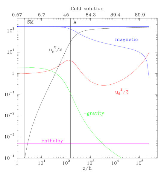
Figure 13: Profiles of various specific energy reservoirs (in $GM/2r_{o}$ units) along a magnetic surface anchored at a radius $r_{o}$, for the cold isothermal solution with $p=0.006$. The SM-point is located at $x_{SM}=z/h=2.08$ and the Alfven point at $x_{A}=151.5$. The thick solid blue line is the sum of all terms and defines the Bernoulli invariant. At the top of the figure, the axis is labelled with the inclination angle (in degrees) from the disk midplane $i=atan(\varepsilon z/h)$.

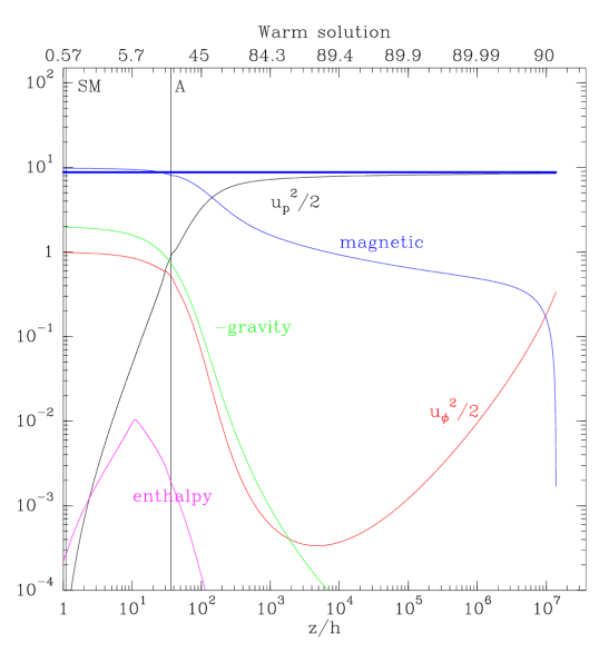
Figure 14: Same as Figure 13, but for the best warm ($\varepsilon=0.01,\,\,p=0.1$) solution. The SM-point is located at $x_{SM}=1.1$ and the Alfven point at $x_{A}=36.2$. Note the drastic decrease of the enthalpy due to the adiabatic cooling, once the heating term vanishes.

References

- Arnaud (1996) Arnaud, K. A. 1996, ASPC, 101, 17
- Blandford & Payne (1982) Blandford, R. D.; Payne, D. G. 1982, MNRAS, 199, 883
- Blum et al. (2010) Blum, J. L.; Miller, J. M.; Cackett, E.; Yamaoka, K.; Takahashi, H.; Raymond, J.; Reynolds, C. S.; Fabian, A. C. 2010, ApJ, 713, 1244
- Casse & Ferreira (2000a) Casse, F.; Ferreira, J. 2000, A&A, 353, 1115
- Casse & Ferreira (2000b) Casse, F.; Ferreira, J. 2000, A&A, 361, 1178
- Chakravorty et al. (2008) Chakravorty, S., Kembhavi, A.K., Elvis, M. & Ferland, G., Badnell, N. R. 2008, MNRAS, 384L, 24
- Chakravorty et al. (2009) Chakravorty, S., Kembhavi, A.K., Elvis, M. & Ferland, G., 2009, MNRAS, 393, 83
- Chakravorty et al. (2012) Chakravorty, S., Misra, R., Elvis, M., Kembhavi, A.K., & Ferland, G., 2009, MNRAS, 393, 83
- Chakravorty et al. (2013) Chakravorty, S., Lee, J. C., Neilsen, J. 2013, MNRAS, 436, 560
- Contopoulos & Lovelace (1994) Contopoulos, J., & Lovelace, R. V. E. 1994, ApJ, 429, 139
- Diaz Trigo et al. (2013) Diaz Trigo, M; Miller-Jones, J.C.A.; Migliari, S; Broderick, J.W.; Tzioumis, T; 2013, Nature, 504, 260
- Ferland et al. (1998) Ferland, G. J.; Korista, K. T.; Verner, D. A.; Ferguson, J. W.; Kingdon, J. B.; Verner, E. M. 1998, PASP, 110, 761
- Ferreira (1993) Ferreira, J., & Pelletier, G. 1993, A&A, 276, 625
- Ferreira (1995) Ferreira, J.; Pelletier, G. 1995, A&A, 295, 807
- Ferreira (1997) Ferreira, J. 1997, A&A, 319, 340
- Ferreira (2004) Ferreira, J.; Casse, F. 2004, ApJ, 601L, 139
- Ferreira et al. (2006) Ferreira, J.; Petrucci, P.-O.; Henri, G.; Saugé, L.; Pelletier, G. 2006, A&A, 447, 813
- Frank, King & Raine (2002) Frank, J., King, A., & Raine, D. 2002, Accretion Power in Astrophysics (3rd ed.; Cambridge: Cambridge Univ. Press)
- Fukumura et al. (2010a) Fukumura, K.; Kazanas, D.; Contopoulos, I.; Behar, E. 2010, ApJ, 715, 636
- Fukumura et al. (2010b) Fukumura, K.; Kazanas, D.; Contopoulos, I.; Behar, E. 2010, ApJ, 723L, 228
- Fukumura et al. (2014) Fukumura, K.; Tombesi, F.; Kazanas, D.; Shrader, C.; Behar, E.; Contopoulos, I. 2014, ApJ, 780, 120
- Fukumura et al. (2015) Fukumura, K.; Tombesi, F.; Kazanas, D.; Shrader, C.; Behar, E.; Contopoulos, I. 2015, ApJ, 805, 17
- Garcia et al. (2001) Garcia, P. J. V.; Ferreira, J.; Cabrit, S.; Binette, L. 2001, A&A, 377, 589
- Higginbottom & Proga (2015) Higginbottom, N.; Proga, D. 2015, ApJ, 807, 107
- Kallman et al. (2009) Kallman, T. R.; Bautista, M. A.; Goriely, S.; Mendoza, C.; Miller, J. M.; Palmeri, P.; Quinet, P.; Raymond, J. 2009, ApJ, 701, 865
- King et al. (2012) King, A. L. et al. 2012, ApJ, 746L, 20
- Kubota et al. (2007) Kubota et al. 2007, PASJ, 59S, 185
- Lee et al. (2002) Lee, J. C. and Reynolds, C. S. and Remillard, R. and Schulz, N. S. and Blackman, E. G. and Fabian, A. C. 2002, ApJ, 567, 1102
- Mitsuda et al. (1984) Mitsuda, K. et al. 1984, PASJ, 36, 741
- Makishima et al. (1987) Makishima, K.; Maejima, Y.; Mitsuda, K.; Bradt, H. V.; Remillard, R. A.; Tuohy, I. R.; Hoshi, R.; Nakagawa, M. 1986, ApJ, 308, 635
- Miller et al. (2004) Miller et al. 2004, ApJ, 601, 450
- Miller et al. (2006) Miller, J. M.; Raymond, J.; Homan, J.; Fabian, A. C.; Steeghs, D.; Wijnands, R.; Rupen, M.; Charles, P.; van der Klis, M.; Lewin, W. H. G. 2006, ApJ, 646, 394
- Miller et al. (2008) Miller, J. M. and Raymond, J and Reynolds, C. S. and Fabian, A. C. and Kallman, T. R. and Homan, J. 2008, ApJ, 680, 1359
- Miller et al. (2012) Miller et al. 2012, ApJ, 759L, 6
- Morrison & McCammon (1983) Morrison, R.; McCammon, D. 1983, ApJ 270, 119
- Neilsen & Lee (2009) Neilsen, J; Lee, J. C. 2009, Natur, 458, 481
- Neilsen et al. (2011) Neilsen, J.; Remillard, R. A.; Lee, J. C. 2011, ApJ, 737, 69
- Neilsen & Homan (2012) Neilsen, J.; Homan, J. arXiv1202.6053
- Peterson (1997) Peterson, B. M. 1997, An Introduction to Active Galactic Nuclei. Cambridge Univ. Press, Cambridge.
- Petrucci et al. (2010) Petrucci, Pierre-Olivier; Ferreira, Jonathan; Henri, Gilles; Malzac, J.; Foellmi, C. 2010, A&A, 522, 38
- Ponti et al. (2014) Ponti, G.; Munoz-Darias, T; Fender, R.P. 2014, MNRAS, 444, 1829
- Ponti et al. (2012) Ponti, G.; Fender, R. P.; Begelman, M. C.; Dunn, R. J. H.; Neilsen, J.; Coriat, M. 2012, MNRAS, 422L, 11
- Remillard & McClintock (2006) Remillard, R. A. and McClintock, J. E. 2006, Annu. Rev. Astron. Astrophys. 44, 49
- Schulz & Brandt (2002) Schulz, N. S.; Brandt, W. N. 2002, ApJ, 572, 971
- Tarter et al. (1969) Tarter, C.B., Tucker, W. & Salpeter, E.E., 1969, ApJ 156, 943
- Ueda et al. (2004) Ueda, Y.; Murakami, H.; Yamaoka, K.; Dotani, T.; Ebisawa, K. 2004, ApJ, 609, 325
- Ueda et al. (2009) Ueda, Y. and Yamaoka, K. and Remillard R. A. 2009, ApJ, 695, 888.
- Ueda et al. (2010) Ueda, Y. et al. 2010, ApJ, 713, 257