MSSM from F-theory SU(5) with Klein Monodromy

Miguel Crispim Romão,^⋆ Athanasios Karozas^† , Stephen F. King^⋆ , George K. Leontaris^† , Andrew K. Meadowcroft^⋆

^⋆ Physics and Astronomy, University of Southampton,

SO17 1BJ Southampton, United Kingdom

^† Physics Department, Theory Division, Ioannina University,

GR-45110 Ioannina, Greece

We revisit a class of $SU(5)$ SUSY GUT models which arise in the context of the spectral cover with Klein Group monodromy $V_{4}=Z_{2}\times Z_{2}$. We show that $Z_{2}$ matter parities can be realised via new geometric symmetries respected by the spectral cover. We discuss a particular example of this kind, where the low energy effective theory below the GUT scale is just the MSSM with no exotics and standard matter parity, extended by the seesaw mechanism with two right-handed neutrinos.

1 Introduction

Over the last decades string theory GUTs have aroused considerable interest. Recent progress has been focused in F-theory [1, 2] effective models [3]-[7] which incorporate several constraints attributed to the topological properties of the compactified space. Indeed, in this context the gauge symmetries are associated to the singularities of the elliptically fibred compactification manifold. As such, GUT symmetries are obtained as a subgroup of $E_{8}$ and the matter content emerges from the decomposition of the $E_{8}$-adjoint representation (for reviews see [8]).

As is well known, GUT symmetries, have several interesting features such as the unification of gauge couplings and the accommodation of fermions in simple representations. Yet, they fail to explain the fermion mass hierarchy and more generally, to impose sufficient constraints on the superpotential terms. Hence, depending on the specific model, several rare processes -including proton decay- are not adequately suppressed. We may infer that, a realistic description of the observed low energy physics world, requires the existence of additional symmetry structure of the effective model, beyond the simple GUT group.

Experimental observations on limits regarding exotic processes (such as baryon and lepton number as well as flavour violating cases) and in particular neutrino physics seem to be nicely explained when the Standard Model or certain GUTs are extended to include abelian and discrete symmetries. On purely phenomenological grounds, $U(1)$ as well as non-abelian discrete symmetries such as $A_{n},S_{n},SLP_{2}(n)$ and so on, have already been successfully implemented. However, in this context there is no principle to single out the family symmetry group from the enormous number of possible finite groups. Moreover, the choice of the scalar spectrum and the Higgs vev alignments introduce another source of arbitrariness in the models.

In contrast to the above picture, F-theory constructions offer an interesting framework for restricting both the gauge (GUT and discrete) symmetries as well as the available Higgs sector. In the elliptic fibration we end up with an 8-dimensional theory with a gauge group of ADE type. In this work we will focus in the simplest unified symmetry which is $SU(5)$ GUT. In the present geometric picture, the $SU(5)$ GUT is supported by 7-branes wrapping an appropriate (del Pezzo) surface $S$ on the internal manifold, while the number of chiral states is given in terms of a topological index formula. Moreover, there is no use of adjoint Higgs representations since the breaking down to the Standard Model symmetry can occur by turning on a non-trivial $U(1)_{Y}$ flux along the hypercharge generator [4]. At the same time this mechanism determines exactly the Standard Model matter content. Further, if the flux parameters are judiciously chosen they may provide a solution to the well known doublet triplet splitting problem of the Higgs sector. In short, in F-theory one can in principle develop all those necessary tools to determine the GUT group and predict the matter content of the effective theory.

In the present work we will revisit a class of $SU(5)$ SUSY GUT models which arise in the context of the spectral cover. The reason is that the recent developments in F-theory provide now a clearer insight and a better perspective of these constructions. For example, developments on computations of the Yukawa couplings[9]-[19] have shown that a reasonable mass hierarchy and mixing may arise even if more than one of the fermion families reside on the same matter curve. This implies that effective models left over with only a few matter curves after certain monodromy identifications could be viable and it would be worth reconsidering them. More specifically, we will consider the case of the Klein Group monodromy $V_{4}=Z_{2}\times Z_{2}$ [22, 23, 24, 26]. Interestingly, with this particular spectral cover, there are two main ways to implement its monodromy action, depending on whether $V_{4}$ is a transitive or non-transitive subgroup of $S_{4}$. A significant part of the present work will be devoted to the viability of the corresponding two kinds of effective models. Another ingredient related to the predictability of the model, is the implementation of R-parity conservation, or equivalently a $Z_{2}$ Matter Parity, which can be realised with the introduction of new geometric symmetries [11] respected from the spectral cover. In view of these interesting features, we also investigate in more detail the superpotential, computing higher non-renormalisable corrections, analysing the D and F-flatness conditions and so on.

The paper is organised as follows. In section 2 we give a short description of the derivation of $SU(5)$ GUT in the context of F-theory. In section 3 we describe the action of monodromies and their role in model building. We further focus on the Klein Group monodromy and the corresponding spectral cover factorisations which is our main concern in the present work. In section 4 we review a few well known mathematical results and theorems which will be used in model building of the subsequent sections. In section 5 we discuss effective field theory models with Klein Group monodromy and implement the idea of matter parity of geometric origin. Section 6 deals with the particle spectrum, the Yukawa sector and other properties and predictions of the effective standard model obtained from the above analysis. Finally we present our conclusions in section 7.

2 The origin of SU(5) in F-theory

In this section we explain the main setup of these class of models. Focusing in the case under consideration, i.e. the GUT $SU(5)$, the effective four dimensional model can be reached from the maximal $E_{8}$ gauge symmetry through the decomposition

$$E_{8}\supset SU(5)_{GUT}\times SU(5)_{\perp}$$

In the elliptic fibration, we know that an ${SU(5)}$ singularity is described by the Tate equation

$$y^{2}=x^{3}+b_{0}z^{5}+b_{2}xz^{3}+b_{3}yz^{2}+b_{4}x^{2}z+b_{5}xy$$ (2.1)

where the homologies of the coefficients in the above equation are given by:

$$[b_{k}] =\eta-kc_{1}$$

$$\eta =6c_{1}-t$$

where $c_{1}$ and $t$ are the Chern classes of the Tangent and Normal bundles respectively.

The first $SU(5)$ is defining the GUT group of the effective theory, the second $SU(5)_{\perp}$ incorporates additional symmetries of the effective theory while it can be described in the context of the spectral cover. Indeed, in this picture, one can depict the non-abelian Higgs bundle in terms of the adjoint scalar field configuration [6] and work with the Higgs eigenvalues and eigenvectors. For $SU(n)$ these emerge as roots of a characteristic polynomial of $n$-th degree. Thus the $SU(5)$ spectral surface $C_{5}$ is represented by the fifth order polynomial

$${C_{5}}=b_{0}s^{5}+b_{1}s^{4}+b_{2}s^{3}+b_{3}s^{2}+b_{4}s+b_{5}\,=\,b_{0}\prod^{5}_{i=1}(s-t_{i})$$ (2.2)

Since the roots are associated to the $SU(5)$ Cartan subalgebra their sum is zero, $\sum_{i}t_{i}=0$, thus we have put $b_{1}=0$.

The $5+\bar{5}$ and $10+\overline{10}$ representations are found at certain ehnancements of the $SU(5)$ singularity. In particular, for this purpose the relevant quantities are [6]

$${\cal P}_{10} = b_{5}=\prod_{i}t_{i}$$ (2.3)

$${\cal P}_{5} = b_{3}^{2}b_{4}-b_{2}b_{3}b_{5}+b_{0}b_{5}^{2}\propto\prod_{i\neq j}(t_{i}+t_{j})$$ (2.4)

At the ${\cal P}_{10}=0$ locus the enhanced singularity is $SO(10)$ and the intersection defines the matter curve accommodating the $10$’s. Fiveplets are found at a matter curve defined at an $SU(6)$ enhancement associated to the locus ${\cal P}_{5}=0$.

In practive, we are interested in phenomenologically viable cases where the spectral cover splits in several pieces. Consider for example the splitting expressed through the breaking chain

$$E_{8}\to SU(5)\times SU(5)\to SU(5)\times U(1)^{4}$$

where we assumed breaking of $SU(5)_{\perp}$ along the Cartan, $\sum_{i}t_{i}=0$. The presence of four $U(1)$’s in the effective theory leaves no room for a viable superpotential, since many of the required terms, including the top Yukawa coupling, are not allowed. Nevertheless, monodromies imply various kinds of symmetries among the roots $t_{i}$ of the spectral cover polynomial which can be used to relax these tight constraints. The particular relations among these roots depend on the details of the compactification and the geometrical properties of the internal manifold. All possible ways fall into some Galois group which in the case of $SU(5)_{\perp}$ is a subgroup of the corresponding Weyl group, i.e., the group $S_{5}$ of all possible permutations of the five Cartan weights $t_{i}$. It is obvious that there are several options and each of them leads to models with completely different properties and predictions of the effective field theory. Before starting our investigations on the effective models derived in the context of the aforementioned monodromy, we will analyse these issues in the next section.

3 The Importance of Monodromy

For the $SU(5)_{GUT}$ model, we have seen that any possible remnant symmetries (embedable in the $E_{8}$ singularity) must be contained in $SU(5)_{\perp}$. We have already explained that in the spectral cover approach we quotient the theory by the action of a finite group [22] which is expected to descend from a geometrical symmetry of the compactification. Starting form an $C_{5}$ spectral cover, the local field theory is determined by the $SU(5)$ GUT group and the Cartan subalgebra of $SU(5)_{\perp}$ modulo the Weyl group $W({\tiny SU(5)_{\perp}})$. This is the group $S_{5}$, the permutation symmetry of five elements which in the present case correspond to the Cartan weights $t_{1,\dots 5}$.

Depending on the geometry of the manifold, $C_{5}$ may slit to several factors

$$C_{5}=\prod_{j}C_{j}$$

For the present work, we will assume two cases where the compactification geometry implies the splitting of the spectral cover to $C_{5}\to C_{4}\times C_{1}$ and $C_{5}\to C_{2}\times C_{2}^{\prime}\times C_{1}$. Assuming the splitting $C_{5}\to C_{4}\times C_{1}$, the permutation takes place between the four roots, say $t_{1,2,3,4}$, and the corresponding Weyl group is $S_{4}$. Notwithstanding, under specific geometries to be discussed in the subsequent sections, the monodromy may be described by the Klein group $V_{4}\in S_{4}$. The latter might be either transitive or non transitive. This second case implies the spectral cover factorisation $C_{4}\to C_{2}\times C_{2}^{\prime}$. As a result, there are two non-trivial identifications acting on the pairs $(t_{1},t_{2})$ and $(t_{3},t_{4})$ respectively while both are described by the Weyl group $W(SU(2)_{\perp})\sim S_{2}$. Since $S_{2}\sim Z_{2}$, we conclude that in this case the monodromy action is the non-transitive Klein group $Z_{2}\times Z_{2}$. Next, we will analyse the basic features of these two spectral cover factorisations.

3.1 $S_{4}$ Subgroups and Monodromy Actions

The group of all permutations of four elements, $S_{4}$, has a total of $24$ elements. These include 2,3,4 and 2+2-cycles, all of which are listed in Table 1. These cycles form a total of 30 subgroups of $S_{4}$, shown in Figure 1. Of these there are those subgroups that are transitive subgroups of $S_{4}$: the whole group, $A_{4}$, $D_{4}$, $Z_{4}$ and the Klein group.

We focus now in compactification geometries consistent with the Klein group monodromy $V_{4}=Z_{2}\times Z_{2}$. We observe that there are three non-transitive $V_{4}$ subgroups within $S_{4}$ and only one transitive subgroup. This transitive Klein group is the subgroup of the $A_{4}$ subgroup. Considering Table 1, one can see that $A_{4}$ is the group of all even permutations of four elements and the transitive $V_{4}$ is that group excluding 3-cycles. The significance of this is that in the case of Galois theory, to be discussed in Section 4, the transitive subgroups $A_{4}$ and $V_{4}$ are necessarily irreducible quartic polynomials, while the non-transitive $V_{4}$ subgroups of $S_{4}$ should be reducible.

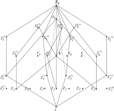
Figure 1: Pictorial summary of the subgroups of $S_{4}$, the group of all permutations of four elements - representative of the symmetries of a cube.

	$S_{4}$ cycles	Transitive $A_{4}$	Transitive $V_{4}$
4-cycles	$(1234)$, $(1243)$, $(1324)$, $(1342)$, $(1423)$, $(1432)$	No	No
3-cycles	$(123)$, $(124)$, $(132)$, $(134)$, $(142)$, $(143)$, $(234)$, $(243)$	Yes	No
2+2-cycles	$(12)(34)$, $(13)(24)$, $(14)(23)$	Yes	Yes
2-cycles	$(12)$, $(13)$, $(14)$, $(23)$, $(24)$, $(34)$	No	No
1-cycles	$e$	Yes	Yes

Table 1: A summary of the permutation cycles of $S_{4}$, categorised by cycle size and whether or not those cycles are contained within the transitive subgroups $A_{4}$ and $V_{4}$. This also shows that $V_{4}$ is necessarily a transitive subgroup of $A_{4}$, since it contains all the $2+2$-cycles of $A_{4}$ and the identity only.

In terms of group elements, the Klein group that is transitive in $S_{4}$ has the elements:

$$\{(1),(12)(34),(13)(24),(14)(23)\}$$ (3.1)

which are the 2+2-cycles shown in Table 1 along with the identity. On the other hand, the non-transitive Klein groups within $S_{4}$ are isomorphic to the subgroup containing the elements:

$$V_{4}=\{(1),(12),(34),(12)(34)\}$$ (3.2)

The distinction here is that the group elements are not all within one cycle, since we have two 2-cycles and one 2+2-cycle. These types of subgroup must lead to a factorisation of the quartic polynomial, as we shall discuss in Section 4. Referring to Figure 1, these Klein groups are the nodes disconnected from the web, while the central $V_{4}$ is the transitive group.

3.2 Spectral cover factorisation

In this section we will discuss the two possible factorisations of the spectral surface compatible with a Klein Group monodromy, in accordance with the previous analysis. In particular, we shall be examining the implications of a monodromy action that is a subgroup of $S_{4}$ - the most general monodromy action relating four weights. In particular we shall be interested in the chain of subgroups $S_{4}\rightarrow A_{4}\rightarrow V_{4}$, which we shall treat as a problem in Galois theory.

3.2.1 ${\mathcal{C}_{4}}$ spectral cover

This set of monodromy actions require the spectral cover of Equation (2.2) to split into a linear part and a quartic part:

$${\mathcal{C}_{5}} \rightarrow{\mathcal{C}_{4}\times C_{1}}$$ (3.3)

$${\mathcal{C}_{5}} \rightarrow(a_{5}s^{4}+a_{4}s^{3}+a_{3}s^{2}+a_{2}s+a_{1})(a_{6}+a_{7}s)$$ (3.4)

The $b_{1}=0$ condition must be enforced for $SU(5)$ tracelessness. This can be solved by consistency in Equation (3.4),

$$b_{1}=a_{5}a_{6}+a_{4}a_{7}=0\,.$$ (3.5)

Let us introduce a new section $a_{0}$, enabling one to write a general solution of the form:

$$a_{4} =\pm a_{0}a_{6}$$

$$a_{5} =\mp a_{0}a_{7}$$

Upon making this substitution, the defining equations for the matter curves are:

$${\mathcal{C}_{5}\,:} =a_{1}a_{6}$$ (3.6)

$${\mathcal{C}_{10}\,:} =(a_{2}^{2}a_{7}+a_{2}a_{3}a_{6}\mp a_{0}a_{1}a_{6}^{2})(a_{3}a_{6}^{2}+(a_{2}a_{6}+a_{1}a_{7})a_{7})$$ (3.7)

which is the most general, pertaining to an $S_{4}$ monodromy action on the roots. By consistency between Equation (3.4) and Equation (2.2), we can calculate that the homologies of the coefficients are:

$$[a_{i}] =\eta-(i-6)c_{1}-\chi$$

$$i =1,2,3,4,5$$

$$[a_{6}] =\chi$$

$$[a_{7}] =c_{1}+\chi$$

$$[a_{0}] =\eta-2(c_{1}+\chi)$$

3.2.2 The $C_{2}\times C_{2}^{\prime}\times C_{1}$ case

If the $V_{4}$ actions are not derived as transitive subgroups of $S_{4}$, then the Klein group is isomorphic to:

$$A_{4}\not\supset V_{4}:\,\,\{(1),(12),(12)(34),(34)\}$$ (3.8)

This is not contained in $A_{4}$, but is admissible from the spectral cover in the form of a monodromy $C_{5}\rightarrow C_{2}\times C_{2}^{\prime}\times C_{1}$.

Then, the ${\bf 10}\in SU(5)$ GUT (${\bf}\in SU(5)_{\perp}$) spectral cover reads

$$C_{5}:(a_{1}+a_{2}s+a_{3}s^{2})(a_{4}+a_{5}s+a_{6}s^{2})(a_{7}+a_{8}s)$$ (3.9)

We may now match the coefficients of this polynomial in each order in $s$ to the ones of the spectral cover with the $b_{k}$ coefficients:

$$b_{0} =a_{368}$$

$$b_{1} =a_{367}+a_{358}+a_{268}$$

$$b_{2} =a_{357}+a_{267}+a_{348}+a_{258}+a_{168}$$ (3.10)

$$b_{3} =a_{347}+a_{257}+a_{167}+a_{248}+a_{158}$$

$$b_{4} =a_{247}+a_{157}+a_{148}$$

$$b_{5} =a_{147}$$

following the notation $a_{ijk}=a_{i}a_{j}a_{k}$ in [23]. In order to find the homology classes of the new coefficients $a_{i}$, we match the coefficients of the above polynomial in each order in $s$ to the ones of Equation (2.2) such that we get relations of the form $b_{k}=b_{k}(a_{i})$.

Comparing to the homologies of the unsplit spectral cover, a solution for the above can be found for the homologies of $a_{i}$. Notice, though, that we have 6 well defined homology classes for $b_{j}$ with only 8 $a_{i}$ coefficients, therefore the homologies of $a_{i}$ are defined up to two homology classes:

$$[a_{n=1,2,3}] =\chi_{1}+(n-3)c_{1}$$

$$[a_{n=4,5,6}] =\chi_{2}+(n-6)c_{1}$$ (3.11)

$$[a_{n=7,8}] =\eta+(n-8)c_{1}-\chi_{1}-\chi_{2}$$

We have to enforce the $SU(5)$ tracelessness condition, $b_{1}=0$. An Ansatz for the solution was put forward in [23],

$$a_{2} =-c(a_{6}a_{7}+a_{5}a_{8})$$

$$a_{3} =ca_{6}a_{8}$$ (3.12)

which introduces a new section, $c$, whose homology class is completely defined by

$$[c]=-\eta+2\chi_{1}$$ (3.13)

With this anstaz for the solution of the splitting of spectral cover, $P_{10}$ reads

$$P_{10}=a_{1}a_{4}a_{7}$$ (3.14)

while the $P_{5}$ splits into

$$P_{5}= a_{5}(a_{6}a_{7}+a_{5}a_{8})(a_{6}a_{7}^{2}+a_{8}(a_{5}a_{7}+a_{4}a_{8}))(a_{1}-a_{5}a_{7}c)$$ (3.15)

$$(a_{1}^{2}-a_{1}(a_{5}a_{7}+2a_{4}a_{8})c+a_{4}(a_{6}a_{7}^{2}+a_{8}(a_{5}a_{7}+a_{4}a_{8}))c^{2}),$$ (3.16)

An extended analysis of this interesting case will be presented in the subsequent sections.

4 A little bit of Galois theory

So far, we have outlined the properties of the most general spectral cover with a monodromy action acting on four of the roots of the perpendicular $SU(5)$ group. This monodromy action is the Weyl group $S_{4}$, however a subgroup is equally admissible as the action. Transitive subgroups are subject to the theorems of Galois theory, which will allow us to determine what properties the coefficients of the quartic factor of Equation (3.4) must have in order to have roots with a particular symmetry [36]-[39]. In this paper we shall focus on the Klein group, $V_{4}\cong Z_{2}\times Z_{2}$. As already mentioned, the transitive $V_{4}$ subgroup of $S_{4}$ is contained within the $A_{4}$ subgroup of $S_{4}$, and so shall share some of the same requirements on the coefficients.

While Galois theory is a field with an extensive literature to appreciate, in the current work we need only reference a handful of key theorems. We shall omit proofs for these theorems as they are readily available in the literature and are not required for the purpose at hand.

Theorem 1.

Let $K$ be a field with characteristic different than $2$, and let $f(X)$ be a separable, polynomial in $K(X)$ of degree $n$.

• If $f(X)$ is irreducible in $K(X)$ then its Galois group over $K$ has order divisible by $n$.

• The polynomial $f(X)$ is irreducible in $K(X)$ if and only if its Galois group over $K$ is a transitive subgroup of $S_{n}$.

This first theorem offers the key point that any polynomial of degree $n$, that has non-degenerate roots, but cannot be factorised into polynomials of lower order with coefficients remaining in the same field must necessarily have a Galois group relating the roots that is $S_{n}$ or a transitive subgroup thereof.

Theorem 2.

Let $K$ be a field with characteristic different than $2$, and let $f(X)$ be a separable, polynomial in $K(X)$ of degree $n$. Then the Galois group of $f(X)$ over $K$ is a subgroup of $A_{n}$ if and only if the discriminant of $f$ is a square in $K$.

As already stated, we are interested specifically in transitive $V_{4}$ subgroups. Theorem 2 gives us the requirement for a Galois group that is $A_{4}$ or its transitive subgroup $V_{4}$ - both of which are transitive in $S_{4}$. Note that no condition imposed on the coefficients of the spectral cover should split the polynomial ($C_{4}\to C_{2}\times C_{2}$), due to Theorem 1. We also know by Theorem 2 that both $V_{4}$ and $A_{4}$ occur when the discriminant of the polynomial is a square, so we necessarily require another mechanism to distinguish the two.

4.1 The Cubic Resolvent

The so-called Cubic Resolvent, is an expression for a cubic polynomial in terms of the roots of the original quartic polynomial we are attempting to classify. The roots of the cubic resolvent are defined to be,

$$x_{1}=(t_{1}t_{2}+t_{3}t_{4}),\,x_{2}=(t_{1}t_{3}+t_{2}t_{4}),\,x_{3}=(t_{1}t_{4}+t_{2}t_{3})$$ (4.1)

and one can see that under any permutation of $S_{4}$ these roots transform between one another. However, in the event that the polynomial has roots with a Galois group relation that is a subgroup of $S_{4}$, the roots need not all lie within the same orbit. The resolvent itself is defined trivially as:

$$(x-(t_{1}t_{2}+t_{3}t_{4}))(x-(t_{1}t_{3}+t_{1}t_{4}))(x-(t_{1}t_{4}+t_{3}t_{2}))=g_{3}x^{3}+g_{2}x^{2}+g_{1}x+g_{0}$$ (4.2)

The coefficients of this equation can be determined by relating of the roots to the original ${\mathcal{C}_{4}}$ coefficients. This resulting polynomial is:

$$g(x)=a_{5}^{3}x^{3}-a_{3}a_{5}^{2}x^{2}+\left(a_{2}a_{4}-4a_{1}a_{5}\right)a_{5}x-a_{2}^{2}a_{5}+4a_{1}a_{3}a_{5}-a_{1}a_{4}^{2}$$ (4.3)

Note that this may be further simplified by making the identification $y=a_{5}x$.

$$g(y)=y^{3}-a_{3}y^{2}+\left(a_{2}a_{4}-4a_{1}a_{5}\right)y-a_{2}^{2}a_{5}+4a_{1}a_{3}a_{5}-a_{1}a_{4}^{2}$$ (4.4)

If the cubic resolvent is factorisable in the field $K$, then the Galois group does not contain any three cycles. For example, if the Galois group is $V_{4}$, then the roots will transform only under the 2+2-cycles:

$$V_{4}\subset A_{4}=\{(1),(12)(34),(13)(24),(14)(23)\}\,.$$ (4.5)

Each of these actions leaves the first of the roots in Equation (4.1) invariant, thus implying that the cubic resolvent is reducible in this case. If the Galois group were $A_{4}$, the 3-cycles present in the group would interchange all three roots, so the cubic resolvent is necessarily irreducible. This leads us to a third theorem, which classifies all the Galois groups of an irreducible quartic polynomial (see also Table 2).

Theorem 3.

The Galois group of a quartic polynomial $f(x)\in K$, can be described in terms of whether or not the discriminant of $f$ is a square in $K$ and whether or not the cubic resolvent of $f$ is reducible in $K$.

Group	Discriminant	Cubic Resolvent
$S_{4}$	$\Delta\neq\delta^{2}$	Irreducible
$A_{4}$	$\Delta=\delta^{2}$	Irreducible
$D_{4}$/$Z_{4}$	$\Delta\neq\delta^{2}$	Reducible
$V_{4}$	$\Delta=\delta^{2}$	Reducible

Table 2: A summary of the conditions on the partially symmetric polynomials of the roots and their corresponding Galois group.

5 Klein monodromy and the origin of matter parity

In this section we will analyse a class of four-dimensional effective models obtained under the assumption that the compactification geometry induces a $Z_{2}\times Z_{2}$ monodromy. As we have seen in the previous section, there are two distinct ways to realise this scenario, which depends on whether the corresponding Klein group is transitive or non-transitive. In the present work we will choose to explore the rather promising case where the monodromy Klein group is non-transitive. In other words, this essentially means that the spectral cover admits a $C_{2}\times C_{2}^{\prime}\times C_{1}$ factorisation. The case of a transitive Klein group is more involved and it is not easy to obtain a viable effective model, hence we will consider this issue in a future work.

Hence, turning our attention to the non-transitive case, the basic structure of the model obtained in this case corresponds to one of those initially presented in [22] and subsequently elaborated by other authors [23]-[26]. This model possesses several phenomenologically interesting features and we consider it is worth elaborating it further.

5.1 Analysis of the $Z_{2}\times Z_{2}$ model

To set the stage, we first present a short review of the basic characteristics of the model following mainly the notation of [23]. The $Z_{2}\times Z_{2}$ monodromy case implies a $2+2+1$ splitting of the spectral fifth-degree polynomial which has already been given in (3.9). Under the action (3.8), for each element, either $x_{2}$ and $x_{3}$ roots defined in (4.1) are exchanged or the roots are unchanged.

The effective model is characterised by three distinct $10$ matter curves, and five $5$ matter curves. The matter curves, along with their charges under the perpendicular surviving $U(1)$ and their homology classes are presented in table 3.

Curve	$U(1)$ Charge	Defining Equation	Homology Class
$10_{1}$	$t_{1}$	$a_{1}$	$-2c_{1}+\chi_{1}$
$10_{3}$	$t_{3}$	$a_{4}$	$-2c_{1}+\chi_{2}$
$10_{5}$	$t_{5}$	$a_{7}$	$\eta-c_{1}-\chi_{1}-\chi_{2}$
$5_{1}$	$-2t_{1}$	$a_{6}a_{7}+a_{5}a_{8}$	$\eta-c_{1}-\chi_{1}$
$5_{13}$	$-t_{1}-t_{3}$	$a_{1}^{2}-a_{1}(a_{5}a_{7}+2a_{4}a_{8})c+a_{4}(a_{6}a_{7}^{2}+a_{8}(a_{5}a_{7}+a_{4}a_{8}))c^{2}$	$-4c_{1}+2\chi_{1}$
$5_{15}$	$-t_{1}-t_{5}$	$a_{1}-a_{5}a_{7}c$	$-2c_{1}+\chi_{1}$
$5_{35}$	$-t_{3}-t_{5}$	$a_{6}a_{7}^{2}+a_{8}(a_{5}a_{7}+a_{4}a_{8})$	$2\eta-2c_{1}-2\chi_{1}-\chi_{2}$
$5_{3}$	$-2t_{3}$	$a_{5}$	$-c_{1}+\chi_{2}$

Table 3: Matter curves and their charges and homology classes

Knowing the homology classes associated to each curve allows us to determine the spectrum of the theory through the units of abelian fluxes that pierce the matter curves. Namely, by turning on a flux in the $U(1)_{X}$ directions, we can endow our spectrum with chirality and break the perpendicular group. In order to retain an anomaly free spectrum we need to allow for

$$\sum M_{5}+\sum M_{10}=0,$$ (5.1)

where $M_{5}$ ($M_{10}$) denote $U(1)_{X}$ flux units piercing a certain $5$ ($10$) matter curve.

A non-trivial flux can also be turned on along the Hypercharge. This will allow us to split GUT irreps, which will provide a solution for the doublet-triplet splitting problem. In order for the Hypercharge to remain ubroken, the flux configuration should not allow for a Green-Schwarz mass, which is accomplished by

$$F_{Y}\cdot c_{1}=0,\ F_{Y}\cdot\eta=0.$$ (5.2)

For the new, unspecified, homology classes, $\chi_{1}$ and $\chi_{2}$ we let the flux units piercing them to be

$$F_{Y}\cdot\chi_{1}=N_{1},\ F_{Y}\cdot\chi_{2}=N_{2},$$ (5.3)

where $N_{1}$ and $N_{2}$ are flux units, and are free parameters of the theory.

For a fiveplet, $5$ one can use the above construction as a doublet-triplet splitting solution as

$$n(3,1)_{-1/3}-n(\overline{3},1)_{1/3}=M_{5},$$ (5.4)

$$n(1,2)_{1/2}-n(1,2)_{-1/2}=M_{5}+N,$$ (5.5)

where the states are presented in the SM basis. For a $10$ we have

$$n(3,2)_{1/6}-n(\overline{3},2)_{-1/6}=M_{10},$$ (5.6)

$$n(\overline{3},1)_{-2/3}-n(3,1)_{2/3}=M_{10}-N,$$ (5.7)

$$n(1,1)_{1}-n(1,1)_{-1}=M_{10}+N.$$ (5.8)

In the end, given a value for each $M_{5}$, $M_{10}$, $N_{1}$, $N_{2}$ the spectrum of the theory is fully defined as can be seen in Table 4

Curve	Weight	Homology	$N_{Y}$	$N_{X}$	Spectrum
$10_{1}$	$t_{1}$	$-2c_{1}+\chi_{1}$	$N_{1}$	$M_{10_{1}}$	$M_{10_{1}}Q+(M_{10_{1}}-N_{1})u^{c}+(M_{10_{1}}+N_{1})e^{c}$
$10_{3}$	$t_{3}$	$-2c_{1}+\chi_{2}$	$N_{2}$	$M_{10_{3}}$	$M_{10_{3}}Q+(M_{10_{3}}-N_{2})u^{c}+(M_{10_{3}}+N_{2})e^{c}$
$10_{5}$	$t_{5}$	$\eta-c_{1}-\chi_{1}-\chi_{2}$	$-N_{1}-N_{2}$	$M_{10_{5}}$	$M_{10_{5}}Q+(M_{10_{5}}+N)u^{c}+(M_{10_{5}}-N)e^{c}$
$5_{1}$	$-2t_{1}$	$\eta-c_{1}-\chi_{1}$	$-N_{1}$	$M_{5_{1}}$	$M_{5_{1}}\overline{d^{c}}+(M_{5_{1}}-N_{1})\overline{L}$
$5_{13}$	$-t_{1}-t_{3}$	$-4c_{1}+2\chi_{1}$	$2N_{1}$	$M_{5_{13}}$	$M_{5_{13}}\overline{d^{c}}+(M_{5_{13}}+2N_{1})\overline{L}$
$5_{15}$	$-t_{1}-t_{5}$	$-2c_{1}+\chi_{1}$	$N_{1}$	$M_{5_{15}}$	$M_{5_{15}}\overline{d^{c}}+(M_{5_{15}}+N_{1})\overline{L}$
$5_{35}$	$-t_{3}-t_{5}$	$2\eta-2c_{1}-2\chi_{1}-\chi_{2}$	$-2N_{1}-N_{2}$	$M_{5_{35}}$	$M_{5_{35}}\overline{d^{c}}+(M_{5_{35}}-2N_{1}-N_{2})\overline{L}$
$5_{3}$	$-2t_{3}$	$-c_{1}+\chi_{2}$	$N_{2}$	$M_{5_{3}}$	$M_{5_{3}}\overline{d^{c}}+(M_{5_{3}}+N_{2})\overline{L}$

Table 4: Matter curve spectrum. Note that $N=N_{1}+N_{2}$ has been used as short hand.

5.2 Matter Parity

It was first proposed before [11], in local F Theory constructions there are geometric discrete symmetries of the spectral cover that manifest on the final field theory. To see this note that the spectral cover equation is invariant, up to a phase, under the transformation $\sigma:s\mapsto\sigma(s)$ of the fibration coordinates, such that

$$s \to se^{i\phi}$$ (5.9)

$$b_{k} \to b_{k}e^{i\chi}e^{i(k-6)\phi}.$$ (5.10)

As detailed in [26] this can be associated to a symmetry of the matter fields residing on the various curves. We can use the equations relating $b_{k}\propto a_{l}a_{m}a_{n}$, with $l+m+n=17$, to find the transformation rules of the $a_{k}$ such that the spectral cover equation respects the symmetry (5.10). This implies that the coefficients $a_{n}$ should transform as

$$a_{n}\to e^{i\psi_{n}}e^{i(11/3-n)\phi}a_{n}.$$ (5.11)

We now note that the above transformations can be achieved by a $Z_{N}$ symmetry if $\phi=3\frac{2\pi}{N}$. In that case one can find, by looking at the equations (3.10) for $b_{k}\propto a_{l}a_{m}a_{n}$ that we have

$$\psi_{1} =\psi_{2}=\psi_{3}$$ (5.12)

$$\psi_{4} =\psi_{5}=\psi_{6}$$ (5.13)

$$\psi_{7} =\psi_{8}$$ (5.14)

meaning that there are three distinct cycles, and

$$\chi=\psi_{1}+\psi_{4}+\psi_{7}.$$ (5.15)

Furthermore, the section $c$ introduced to split the matter conditions (3.12) has to transform as

$$c\to e^{i\phi_{c}}c,$$ (5.16)

with

$$\phi_{c}=\psi_{3}-\psi_{6}-\psi_{7}+\left(-\frac{11}{3}+11\right)\phi\quad{,}\quad\phi_{c}=\psi_{2}-\psi_{5}-\psi_{8}+\left(-\frac{11}{3}+11\right)\phi$$ (5.17)

We can now deduce what would be the matter parity assignments for $Z_{2}$ with $\phi=3(2\pi/2)$. Let $p(x)$ be the parity of a section (or products of sections), $x$. We notice that there are relations between the parities of different coefficients, for example one can easily find

$$\frac{p(a_{1})}{p(a_{2})}=-1$$ (5.18)

amongst others, which allow us to find that all parity assignments depend only on three independent parities

$$p(a_{1}) =i$$ (5.19)

$$p(a_{4}) =j$$ (5.20)

$$p(a_{7}) =k$$ (5.21)

$$p(c) =ijk,$$ (5.22)

where we notice that $i^{2}=j^{2}=k^{2}=+$. The parities for each matter curve – both in form of a function of $i,j,k$ and all possible assignments – can are presented in the table 5.

Curve	Charge	Parity	All possible assignments
$10_{1}$	$t_{1}$	$i$	$+$	$-$	$+$	$-$	$+$	$-$	$+$	$-$
$10_{3}$	$t_{3}$	$j$	$+$	$+$	$-$	$-$	$+$	$+$	$-$	$-$
$10_{5}$	$t_{5}$	$k$	$+$	$+$	$+$	$+$	$-$	$-$	$-$	$-$
$5_{1}$	$-2t_{1}$	$jk$	$+$	$+$	$-$	$-$	$-$	$-$	$+$	$+$
$5_{13}$	$-t_{1}-t_{3}$	$+$	$+$	$+$	$+$	$+$	$+$	$+$	$+$	$+$
$5_{15}$	$-t_{1}-t_{5}$	$i$	$+$	$-$	$+$	$-$	$+$	$-$	$+$	$-$
$5_{35}$	$-t_{3}-t_{5}$	$j$	$+$	$+$	$-$	$-$	$+$	$+$	$-$	$-$
$5_{3}$	$-2t_{3}$	$-j$	$-$	$-$	$+$	$+$	$-$	$-$	$+$	$+$

Table 5: All possible matter parity assignments

As such, models from $Z_{2}\times Z_{2}$ are completely specified by the information present in table 6.

Curve	Charge	Matter Parity	Spectrum
$10_{1}$	$t_{1}$	$i$	$M_{10_{1}}Q+(M_{10_{1}}-N_{1})u^{c}+(M_{10_{1}}+N_{1})e^{c}$
$10_{3}$	$t_{3}$	$j$	$M_{10_{3}}Q+(M_{10_{3}}-N_{2})u^{c}+(M_{10_{3}}+N_{2})e^{c}$
$10_{5}$	$t_{5}$	$k$	$M_{10_{5}}Q+(M_{10_{5}}+N_{1}+N_{2})u^{c}+(M_{10_{5}}-N_{1}-N_{2})e^{c}$
$5_{1}$	$-2t_{1}$	$jk$	$M_{5_{1}}\overline{d^{c}}+(M_{5_{1}}-N_{1})\overline{L}$
$5_{13}$	$-t_{1}-t_{3}$	$+$	$M_{5_{13}}\overline{d^{c}}+(M_{5_{13}}+2N_{1})\overline{L}$
$5_{15}$	$-t_{1}-t_{5}$	$i$	$M_{5_{15}}\overline{d^{c}}+(M_{5_{15}}+N_{1})\overline{L}$
$5_{35}$	$-t_{3}-t_{5}$	$j$	$M_{5_{35}}\overline{d^{c}}+(M_{5_{35}}-2N_{1}-N_{2})\overline{L}$
$5_{3}$	$-2t_{3}$	$-j$	$M_{5_{3}}\overline{d^{c}}+(M_{5_{3}}+N_{2})\overline{L}$

Table 6: All the relevant information for model building with $Z_{2}\times Z_{2}$ monodromy

5.3 The Singlets

For the singlets on the GUT surface we start by looking at the splitting equation for singlet states, $P_{0}$. For $SU(5)$ these are found to be

$$P_{0} =3125b_{5}^{4}b_{0}^{4}+256b_{4}^{5}b_{0}^{3}-3750b_{2}b_{3}b_{5}^{3}b_{0}^{3}+2000b_{2}b_{4}^{2}b_{5}^{2}b_{0}^{3}+2250b_{3}^{2}b_{4}b_{5}^{2}b_{0}^{3}-1600b_{3}b_{4}^{3}b_{5}b_{0}^{3}-128b_{2}^{2}b_{4}^{4}b_{0}^{2}$$

$$+144b_{2}b_{3}^{2}b_{4}^{3}b_{0}^{2}-27b_{3}^{4}b_{4}^{2}b_{0}^{2}+825b_{2}^{2}b_{3}^{2}b_{5}^{2}b_{0}^{2}-900b_{2}^{3}b_{4}b_{5}^{2}b_{0}^{2}+108b_{3}^{5}b_{5}b_{0}^{2}+560b_{2}^{2}b_{3}b_{4}^{2}b_{5}b_{0}^{2}-630b_{2}b_{3}^{3}b_{4}b_{5}b_{0}^{2}$$

$$+16b_{2}^{4}b_{4}^{3}b_{0}-4b_{2}^{3}b_{3}^{2}b_{4}^{2}b_{0}+108b_{2}^{5}b_{5}^{2}b_{0}+16b_{2}^{3}b_{3}^{3}b_{5}b_{0}-72b_{2}^{4}b_{3}b_{4}b_{5}b_{0}$$ (5.23)

Applying the solution for the $Z_{2}\times Z_{2}$ monodromy from Eq.(3.11,3.12) the above splits into 13 factors as follows

$$P_{0} =a_{6}^{2}a_{8}^{2}c\left(a_{5}^{2}-4a_{4}a_{6}\right)\left(a_{8}(a_{4}a_{8}-a_{5}a_{7})+a_{6}a_{7}^{2}\right)^{2}$$

$$\left(c(a_{5}a_{8}+a_{6}a_{7})^{2}-4a_{1}a_{6}a_{8}\right)(a_{1}a_{8}+a_{7}c(a_{5}a_{8}+2a_{6}a_{7}))^{2}$$

$$\left(a_{1}^{2}a_{6}+a_{1}c\left(-2a_{4}a_{6}a_{8}+2a_{5}^{2}a_{8}+a_{5}a_{6}a_{7}\right)+a_{4}c^{2}\left(a_{6}a_{8}(a_{4}a_{8}+3a_{5}a_{7})+2a_{5}^{2}a_{8}^{2}+a_{6}^{2}a_{7}^{2}\right)\right)^{2}$$ (5.24)

Their homologies and geometric parities can be founded by applying the results from the previous section, and are presented in Table 7

Equation	Power	Charge	Homology Class	Matter Parity
$a_{6}$	2	$\pm(t_{1}-t_{3})$	$\chi_{2}$	$j$
$a_{8}$	2	$\pm(t_{1}-t_{5})$	$\eta-\chi_{1}-\chi_{2}$	$-k$
$c$	1	$0$	$-\eta+2\chi_{1}$	$ijk$
$a_{5}^{2}-\ldots$	1	$0$	$-2c_{1}+\chi_{2}$	$+$
$a_{8}(a_{4}a_{8}-\ldots$	2	$\pm(t_{3}-t_{5})$	$2\eta-2c_{1}-2\chi_{1}-\chi_{2}$	$j$
$c(a_{5}a_{8}+\ldots$	1	$0$	$\eta-2c_{1}$	$ijk$
$(a_{1}a_{8}+\ldots$	2	$\pm(t_{1}-t_{5})$	$\eta-2c_{1}-\chi_{2}$	$-ik$
$(a_{1}^{2}a_{6}+\ldots$	2	$\pm(t_{1}-t_{3})$	$-4c_{1}+2\chi_{1}+\chi_{2}$	$j$

Table 7: Defining euations, multiplicity, homologies, matter parity, and perpendicular charges of singlet factors

5.4 Application of Geometric Matter Parity

We study now the implementation of the explicit $Z_{2}\times Z_{2}$ monodromy model presented in [23] alongside the matter parity proposed above. The model under consideration is defined by the flux data

$$N_{1}=M_{5_{15}}=M_{5_{35}}=0$$ (5.25)

$$N_{2}=M_{10_{3}}=M_{5_{1}}=1=-M_{10_{5}}=-M_{5_{3}}$$ (5.26)

$$M_{10_{1}}=3=-M_{5_{13}}$$ (5.27)

which leads to the spectrum presented in Table 8 alongside all possible geometric parities.

Curve	Charge	Spectrum	All possible assignments
$10_{1}$	$t_{1}$	$3Q+3u^{c}+3e^{c}$	$+$	$-$	$+$	$-$	$+$	$-$	$+$	$-$
$10_{3}$	$t_{3}$	$Q+2e^{c}$	$+$	$+$	$-$	$-$	$+$	$+$	$-$	$-$
$10_{5}$	$t_{5}$	$-Q-2e^{c}$	$+$	$+$	$+$	$+$	$-$	$-$	$-$	$-$
$5_{1}$	$-2t_{1}$	$D_{u}+H_{u}$	$+$	$+$	$-$	$-$	$-$	$-$	$+$	$+$
$5_{13}$	$-t_{1}-t_{3}$	$-3\overline{d^{c}}-3\overline{L}$	$+$	$+$	$+$	$+$	$+$	$+$	$+$	$+$
$5_{15}$	$-t_{1}-t_{5}$	$0$	$+$	$-$	$+$	$-$	$+$	$-$	$+$	$-$
$5_{35}$	$-t_{3}-t_{5}$	$-\overline{H}_{d}$	$+$	$+$	$-$	$-$	$+$	$+$	$-$	$-$
$5_{3}$	$-2t_{3}$	$-\overline{D}_{d}$	$-$	$-$	$+$	$+$	$-$	$-$	$+$	$+$

Table 8: Spectrum and allowed geometric parities for the $Z_{2}\times Z_{2}$ monodromy model

Name	Charge	All possible assignments
$\theta_{1}$	$\pm(t_{1}-t_{3})$	$+$	$+$	$-$	$-$	$+$	$+$	$-$	$-$
$\theta_{2}$	$\pm(t_{1}-t_{5})$	$-$	$-$	$-$	$-$	$+$	$+$	$+$	$+$
$\theta_{3}$	$0$	$+$	$-$	$-$	$+$	$-$	$+$	$+$	$-$
$\theta_{4}$	$0$	$+$	$+$	$+$	$+$	$+$	$+$	$+$	$+$
$\theta_{5}$	$\pm(t_{3}-t_{5})$	$+$	$+$	$-$	$-$	$+$	$+$	$-$	$-$
$\theta_{6}$	$0$	$+$	$-$	$-$	$+$	$-$	$+$	$+$	$-$
$\theta_{7}$	$\pm(t_{1}-t_{5})$	$-$	$+$	$-$	$+$	$+$	$-$	$+$	$-$
$\theta_{8}$	$\pm(t_{1}-t_{3})$	$+$	$+$	$-$	$-$	$+$	$+$	$-$	$-$

Table 9: Singlet curves and their perpendicular charges and geometric parity

Inspecting Table 8 one can arrive at some conclusions. For example, looking at the spectrum from each curve it’s immediate that all matter is contained in $10_{1}$ and $5_{13}$, while the Higgses come from $5_{1}$ and $5_{35}$, and the rest of the states are exotics that come in vector-like pairs. Immediately we see that there will be R-Parity violating terms since $5_{13}$ has positive parity.

In order to fully describe the model one also has to take into account the singlets, whose perpendicular charges and all possible geometric parities can be seen in Table 9, where we included the same field with its charge conjugated partner in the same row - i.e. $\theta_{i}$ has the same parity as $\overline{\theta}_{i}$.

Of the possible combinations $\{i,j,k\}$ for the geometric parity assignments, the only choices that allow for a tree-level top quark mass are:

$$\{i,j,k\}=\{+,+,+\}$$ (5.28)

$$\{i,j,k\}=\{-,+,+\}$$

$$\{i,j,k\}=\{+,-,-\}$$

$$\{i,j,k\}=\{-,-,-\}$$

The option that most closely resembles the R-parity imposed in the model [23] corresponds to the choice $i=-$, $j=k=+$. However, if R-parity has a geometric origin the parity assignments of matter curves cannot be arbitrarily chosen. Using the Mathematica package presented in [44], it is straight forward to produce the spectrum of operators up to an arbitrary mass dimension. One can readily observe that its implementation allows a number of operators that could cause Bilinear R-Parity Violation (BRPV) at unacceptably high rates. For example, the lowest order operators are:

$$H_{u}L\theta_{1},\,H_{u}L\theta_{8},\,H_{u}L\theta_{1}\theta_{4},\,H_{u}L\theta_{4}\theta_{8},\,H_{u}L\overline{\theta}_{5}\theta_{7}$$ (5.29)

with higher order operators also present, amplifying the scale of the problem. In order to avoid problems, we must forbid vacuum expectations for a number of singlets, especially $\theta_{1}$ and $\theta_{8}$. This does not immediately appear to be a model killing issue, however we must look to the exotic masses. Considering the Higgs triplets $D_{u/d}$, the only mass terms are:

$$D_{u}D_{d}\theta_{1}\theta_{1}\theta_{3},\,D_{u}D_{d}\theta_{1}\theta_{1}\theta_{6},\,D_{u}D_{d}\theta_{1}\theta_{2}\overline{\theta}_{5},\,D_{u}D_{d}\theta_{1}\theta_{3}\theta_{8},\,$$

$$D_{u}D_{d}\theta_{1}\theta_{6}\theta_{8},\,D_{u}D_{d}\theta_{2}\overline{\theta}_{5}\theta_{8},\,D_{u}D_{d}\theta_{3}\theta_{8}\theta_{8},\,D_{u}D_{d}\theta_{6}\theta_{8}\theta_{8}$$ (5.30)

As can be seen each of these terms contains $\theta_{1}$ or $\theta_{8}$. Since these are required to have no vacuum expectation value, it follows that the Higgs triplets cannot become massive. Since this is a highly disfavoured feature, we must rule out this model.

It transpires that in a similar way, all the models with this flux assignment must be ruled out when we apply this geometric parity. This is due to the tension between BRPV terms and exotic masses, which seem to always be at odds in models with this novel parity. This motivates one to search for models without any exotics, as these models will not have any constraining features coming from exotic masses, and we shall analyse one such model in the subsequence.

6 Deriving the MSSM with the seesaw mechanism

The parameter space of models is very large, given the number of reasonable combinations of fluxes, multiplicities and choices of geometric parities. There are a number of ways to narrow the parameter space of any search, for example requing that there be no exotics present in the spectrum, or contriving there to be only one tree-level Yukawa (to enable a heavy top quark), or perhaps allowing only models with standard matter parity be considered. This last option is quite difficult to search for, but can be constructed.

Let us make a choice for the flux parameters that enables this standard matter parity:

$$\{N_{1}=1,N_{2}=0\}$$

$$M_{10_{1}}=-M_{5_{13}}=2$$

$$M_{10_{5}}=-M_{5_{3}}=1$$ (6.1)

$$M_{10_{3}}=M_{5_{1}}=M_{5_{13}}=M_{5_{35}}=0$$

$$i=-j=k=-$$

The matter spectrum of this model is summarised in Table 10. With this choice, Table 9 will select the column with only the singlets $\theta_{7}$ and $\overline{\theta}_{7}$ having a negative matter parity. Provided this singlet does not acquire a vacuum expectation it will then be impossible for Bilinear R-parity violating terms due to the nature of the parity assignments. This will also conveniently give us candidates for right-handed neutrinos, $\theta_{7}$ and $\overline{\theta}_{7}$.

Curve	Charge	Matter Parity	Spectrum
$10_{1}$	$t_{1}$	$-$	$Q_{3}+Q_{2}+u^{c}_{3}+3e^{c}$
$10_{3}$	$t_{3}$	$+$	$-$
$10_{5}$	$t_{5}$	$-$	$Q_{1}+u^{c}_{2}+u^{c}_{1}$
$5_{1}$	$-2t_{1}$	$-$	$-\overline{L}_{1}$
$5_{13}$	$-t_{1}-t_{3}$	$+$	$2H_{u}$
$5_{15}$	$-t_{1}-t_{5}$	$-$	$-\overline{d}_{2}^{c}-\overline{d}_{1}^{c}-\overline{L}_{2}$
$5_{35}$	$-t_{3}-t_{5}$	$+$	$-2\overline{H}_{d}$
$5_{3}$	$-2t_{3}$	$-$	$-\overline{d}^{c}_{3}-\overline{L}_{3}$
$1_{15}=\theta_{7}$	$t_{1}-t_{5}$	$-$	$N_{R}^{a}$
$1_{51}=\overline{\theta}_{7}$	$t_{5}-t_{1}$	$-$	$N_{R}^{b}$

Table 10: Matter content for a model with the standard matter parity arising from a geometric parity assignment.

6.1 Yukawas

Having written down a spectrum that has the phenomenologically preferred R-parity, we must now examine the allowed couplings of the model. The model only allows Yukawa couplings to arise at non-renormalisable levels, however the resulting couplings give rise to rank three mass matrices. This is because the perpendicular group charges must be canceled out in any Yukawa couplings. For example, the Yukawa arising from $10_{1}\cdot 10_{1}\cdot 5_{13}$ has a charge $t_{1}-t_{3}$, which may be canceled by the $\theta_{1/8}$ singlets. Consider the Yukawas of the Top sector,

$$10_{1}\cdot 10_{1}\cdot 5_{13}\cdot(\overline{\theta}_{1}+\overline{\theta}_{8}) \rightarrow(Q_{3}+Q_{2})u_{3}H_{u}(\overline{\theta}_{1}+\overline{\theta}_{8})$$

$$10_{1}\cdot 10_{5}\cdot 5_{13}\cdot\theta_{5} \rightarrow((Q_{3}+Q_{2})(u_{1}+u_{2})+Q_{1}u_{3})H_{u}\theta_{5}$$ (6.2)

$$10_{5}\cdot 10_{5}\cdot 5_{13}\cdot\theta_{2}\cdot\theta_{5} \rightarrow Q_{1}(u_{1}+u_{2})H_{u}\theta_{2}\theta_{5}$$

where the numbers indicate generations (1, 2 and 3). The resulting mass matrix should be rank three, however the terms will not all be created equally and the rank theorem [10] should lead to suppression of operators arising from the same matter curve combination:

$$M_{u,c,t}\sim v_{u}\left(\begin{array}[]{ccc}\epsilon\theta_{2}\theta_{5}&\theta_{2}\theta_{5}&\theta_{5}\\ \epsilon^{2}\theta_{5}&\epsilon\theta_{5}&\epsilon(\overline{\theta}_{1}+\overline{\theta}_{8})\\ \epsilon\theta_{5}&\theta_{5}&\overline{\theta}_{1}+\overline{\theta}_{8}\end{array}\right)$$ (6.3)

where each element of the matrix has some arbitrary coupling constant. We use here $\epsilon$ to denote suppression due to the effects of the Rank Theorem [10] for Yukawas arising from the same GUT operators. The lightest generation will have the lightest mass due to an extra GUT scale suppression arising from the second singlet involved in the Yukawa. There are a large number of corrections at higher orders in singlet VEVs, which we have not included here for brevity. These corrections will also be less significant compared to the lowest order contributions.

In a similar way, the Down-type Yukawa couplings arise as non-renormalisable operators, coming from four different combinations. The operators for this sector often exploit the tracelessness of $SU(5)$, so that the sum of the GUT charges must vanish. The leading order Yukawa operators,

$$10_{1}\cdot\overline{5}_{3}\cdot\overline{5}_{35}\cdot(\theta_{1}+\theta_{8}) \rightarrow(Q_{3}+Q_{2})d_{3}H_{d}(\theta_{1}+\theta_{8})$$

$$10_{1}\cdot\overline{5}_{15}\cdot\overline{5}_{35}\cdot\theta_{5} \rightarrow(Q_{3}+Q_{2})(d_{1}+d_{2})H_{d}\theta_{5}$$ (6.4)

$$10_{5}\cdot\overline{5}_{3}\cdot\overline{5}_{35}\cdot(\theta_{1}+\theta_{8})\theta_{2} \rightarrow Q_{1}d_{3}H_{u}(\theta_{1}+\theta_{8})\theta_{2}$$

$$10_{5}\cdot\overline{5}_{15}\cdot\overline{5}_{35}\cdot\theta_{2}\cdot\theta_{5} \rightarrow Q_{1}(d_{1}+d_{2})H_{u}\theta_{2}\theta_{5}$$

The resulting mass matrix will, like in the Top sector, be a rank three matrix, with a similar form:

$$M_{d,s,b}\sim v_{d}\left(\begin{array}[]{ccc}\epsilon\theta_{2}\theta_{5}&\theta_{2}\theta_{5}&(\theta_{1}+\theta_{8})\theta_{2}\\ \epsilon^{2}\theta_{5}&\epsilon\theta_{5}&\epsilon(\theta_{1}+\theta_{8})\\ \epsilon\theta_{5}&\theta_{5}&\theta_{1}+\theta_{8}\end{array}\right)$$ (6.5)

The structure of the Top and Bottom sectors appears to be quite similar in this model, which should provide a suitable hierarchy to both sectors.

The Charged Leptons will have a different structure to the Bottom-type quarks in this model, due primarily to the fact the $e^{c}_{i}$ matter is localised on one GUT tenplet. The Lepton doublets however all reside on different $\overline{5}$ representations, which will fill out the matrix in a non-trivial way, with the operators:

$$10_{1}\cdot\overline{5}_{3}\cdot\overline{5}_{35}\cdot(\overline{\theta}_{1}+\overline{\theta}_{8}) \rightarrow L_{3}(e^{c}_{1}+e^{c}_{2}+e^{c}_{3})H_{d}(\overline{\theta}_{1}+\overline{\theta}_{8})$$

$$10_{1}\cdot\overline{5}_{15}\cdot\overline{5}_{35}\cdot\theta_{5} \rightarrow L_{2}(e^{c}_{1}+e^{c}_{2}+e^{c}_{3})H_{d}\theta_{5}$$ (6.6)

$$10_{1}\cdot\overline{5}_{1}\cdot\overline{5}_{35}\cdot(\theta_{1}+\theta_{8}) \rightarrow L_{1}(e^{c}_{1}+e^{c}_{2}+e^{c}_{3})H_{d}(\theta_{1}+\theta_{8})$$

The mass matrix for the Charged Lepton sector will be subject to suppressions arising due to the effects discussed above.

6.2 Neutrino Masses

The spectrum contains two singlets that do not have vacuum expectation values, which protects the model from certain classes of dangerous operators. These singlets, $\theta_{7}/\overline{\theta}_{7}$, also serve as candidates for right-handed neutrinos. Let us make the assignment $\theta_{7}=N_{R}^{a}$ and $\overline{\theta}_{7}=N_{R}^{b}$. This gives Dirac masses from two sources, the first of which involve all lepton doublets and $N_{R}^{a}$:

$$\overline{5}_{3}\cdot 5_{13}\cdot\theta_{7}\cdot\overline{\theta}_{5} \rightarrow L_{3}N_{R}^{a}H_{u}\overline{\theta}_{5}$$

$$\overline{5}_{15}\cdot 5_{13}\cdot\theta_{7}\cdot(\overline{\theta}_{1}+\overline{\theta}_{8}) \rightarrow L_{2}N_{R}^{a}H_{u}(\overline{\theta}_{1}+\overline{\theta}_{8})$$ (6.7)

$$\overline{5}_{1}\cdot 5_{13}\cdot\theta_{7}\cdot(\overline{\theta}_{1}+\overline{\theta}_{8})\cdot\theta_{2} \rightarrow L_{1}N_{R}^{a}H_{u}(\overline{\theta}_{1}+\overline{\theta}_{8})\theta_{2}$$

This generates a hierarchy for neutrinos, however the effect will be mitigated by the operators arising from the $N_{R}^{b}$ singlet:

$$\overline{5}_{3}\cdot 5_{13}\cdot\overline{\theta}_{7}\cdot(\overline{\theta}_{1}+\overline{\theta}_{8})\cdot\theta_{2} \rightarrow L_{3}N_{R}^{b}H_{u}(\overline{\theta}_{1}+\overline{\theta}_{8})\theta_{2}$$

$$\overline{5}_{15}\cdot 5_{13}\cdot\overline{\theta}_{7}\cdot\theta_{2}\cdot\theta_{5} \rightarrow L_{2}N_{R}^{b}H_{u}\theta_{2}\theta_{5}$$ (6.8)

$$\overline{5}_{1}\cdot 5_{13}\cdot\overline{\theta}_{7}\cdot\theta_{5} \rightarrow L_{1}N_{R}^{b}H_{u}\theta_{5}$$

If all these Dirac mass operators are present in the low energy spectrum, then the neutrino sector should have masses that mix greatly. This is compatible with our understanding of neutrinos from experiments, which requires large mixing angles compared to the other sectors.

A light mass scale for the neutrinos can be generated using the seesaw mechanism [41], which requires large right-handed Majorana masses to generate light physical left-handed Majorana neutrino mass at low values. The singlets involved in this scenario has perpendicular charges that must be canceled out, as with the quark and charged lepton operators. Fortunately, this can be achieved, in part due to the presence of $\theta_{2}/\overline{\theta}_{2}$, which have the same charge combinations as $N_{R}^{a,b}$. The leading contribution to the mass term will come from the off diagonal $\theta_{7}\overline{\theta}_{7}$ term, however there are diagonal contributions:

$$\frac{\langle\theta_{2}\rangle^{2}}{\Lambda}\overline{\theta}_{7}^{2}\,\,+\,\,\frac{\langle\overline{\theta}_{2}\rangle^{2}}{\Lambda}\theta_{7}^{2}\,\,+\,\,M\theta_{7}\overline{\theta}_{7}$$ (6.9)

Two right-handed neutrinos are sufficient to generate the appropriate physical light masses for the neutrinos required by experimental constraints [42, 43].

6.3 Other Features

An interesting property of this model is the requirement of extra Higgs fields. Due to the flux factors, under doublet-triplet splitting it is necessary to have two copies of the up and down-type Higgs. This insures that the model is free of Higgs colour triplets, $D_{u}/D_{d}$ in the massless spectrum, while also allowing the designation of $+$ parity to Higgs matter curves. As a consequence of this, the $\mu$-term for the Higgs mass would seem to give four Higgs operators of the same mass: $M_{ij}H_{u}^{i}H_{d}^{j}$, with $i,j=1,2$. However, since for both the up and down-types there are two copies on the matter curve, we can call upon the rank theorem [10]. Consider the operator for the $\mu$-term:

$$5_{13}\cdot\overline{5}_{35}\cdot\theta_{2}\rightarrow M_{ij}H_{u}^{i}H_{d}^{j}\rightarrow M\left(\begin{array}[]{cc}\epsilon_{h}^{2}&\epsilon_{h}\\ \epsilon_{h}&1\end{array}\right)\left(\begin{array}[]{c}H_{u}^{1}\\ H_{u}^{2}\end{array}\right)\left(\begin{array}[]{cc}H_{d}^{1}&H_{d}^{2}\end{array}\right)$$ (6.10)

This operator will give a mass that is naturally large for one generation of the Higgs, while the second mass should be suppressed due to non-perturbative effects. This is parameterised by $\epsilon_{h}$, which is required to be sufficiently small as to allow a Higgs to be present at the electroweak scale, while the leading order Higgsl must be heavy enough to remain at a reasonably high scale and not prevent unification. Thus we should have a light Higgs boson as well as a heavier copy that is as of yet undetected.

The spectrum is free of the Higgs colour triplets $D_{u}/D_{d}$, however we must still consider operators of the types $QQQL$ and $d^{c}u^{c}u^{c}e^{c}$, since the colour triplets may appear in the spectrum at the string scale. Of these types of operator, most are forbidden at leading order due to the charges of the perpendicular group. However, one operator is allowed and we must consider this process:

$$10_{1}10_{1}10_{5}\overline{5}_{3}\rightarrow(Q_{3}+Q_{2})(Q_{3}+Q_{2})Q_{1}L_{3}+(u^{c}_{2}+u^{c}_{1})u_{3}^{c}d^{c}_{3}(e^{c}_{1}+e^{c}_{2}+e^{c}_{3})$$ (6.11)

None of the operators arising are solely first generation matter, however due to mixing they may contribute to any proton decay rate. The model in question only has one of each type of Higgs matter curve, which means any colour triplet partners must respect the perpendicular charges of those curves. The result of this requirement is that the vertex between the initial quarks and the $D_{u}$ colour triplet must also include a singlet to balance the charge, with the same requirement for the final vertex. The resulting operator should be suppressed by some high scale where the colour triplets are appearing in the spectrum - $\Lambda_{s}$. The most dangerous contribution of this operator can be assume to be the $Q_{2}Q_{1}Q_{2}L_{3}$ component, which will mix most strongly with the lightest generation. It can be estimated that, given the quark mixing and the mixing structure of the charged Leptons in particular, the suppression scale should be in the region $\sim 10^{4-6}\Lambda_{s}$. This estimate seems to place the suppression of proton decay at too small a value, though not wildly inconsistent.

However, if we consider Figure 2, we can see that while the external legs of this process give an overall adherence to the charges of the perpendicular group charges, the vertices require singlet contributions. For example, the first vertex is $Q_{2}Q_{1}D_{u}\theta_{5}$, which is nonrenormalisable and we cannot write down a series of renormalisable operators to mediate this effective operator. This is because the combination of perpendicular group and GUT charges constrain heavily the operators we can write down, which means proton decay can be seen to be suppressed here by the dynamics as well as the symmetries required by the F-theory formalism. The full determination of the coupling strengths of any process of this type in F-theory should be found through computing the overlap integral of the wavefunctions involved [20], and this will be discussed in upcoming work on R-parity violating processes.

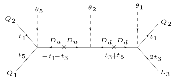
Figure 2: Proton Decay graph

7 Conclusions

We have revisited a class of $SU(5)$ SUSY GUT models which arise in the context of the spectral cover with Klein Group monodromy $V_{4}=Z_{2}\times Z_{2}$. By investigating the symmetry structures of the spectral cover equation and the defining equations of the mater curves it is possible to understand the F-theory geometric origin of matter parity, which has hitherto been just assumed in an ad hoc way. In particular, we have shown how the simplest $Z_{2}$ matter parities can be realised via the new geometric symmetries respected by the spectral cover. By exploiting the various ways that these symmetries can be assigned, there are a large number of possible variants.

We have identified a rather minimal example of this kind, where the low energy effective theory below the GUT scale is just the MSSM with no exotics and standard matter parity. Furthermore, by deriving general properties of the singlet sector, consistent with string vacua, including the D and F-flatness conditions, we were able to identify two singlets, which provide suitable candidates for a two right-handed neutrinos. We were thus able to derive the MSSM extended by a two right-handed neutrino seesaw mechanism. We also computed all baryon and lepton number violating operators emerging from higher non-renormalisable operators and found all dangerous operators to be forbidden.

SFK acknowledges partial support from the STFC Consolidated ST/J000396/1 grant and the European Union FP7 ITN-INVISIBLES (Marie Curie Actions, PITN- GA-2011-289442). AKM is supported by an STFC studentship. MCR acknowledges support from the FCT under the grant SFRH/BD/84234/2012.

Appendix A F-Flatness

The super potential for the singlets involves a total of thirteen fields, which couple in such as way as to cancel all their perpendicular group charges and to have consistent parity.

$$W\supset c_{17}\theta_{1}\overline{\theta}_{1}\theta_{3}+c_{18}\theta_{1}\overline{\theta}_{1}\theta_{4}+c_{19}\theta_{1}\overline{\theta}_{1}\theta_{6}+c_{4}\theta_{1}\overline{\theta}_{1}+c_{20}\theta_{1}\overline{\theta}_{2}\theta_{5}+c_{21}\theta_{1}\theta_{3}\overline{\theta}_{8}+$$

$$c_{22}\theta_{1}\theta_{4}\overline{\theta}_{8}+c_{23}\theta_{1}\theta_{6}\overline{\theta}_{8}+c_{5}\theta_{1}\overline{\theta}_{8}+c_{24}\overline{\theta}_{1}\theta_{2}\overline{\theta}_{5}+c_{25}\overline{\theta}_{1}\theta_{3}\theta_{8}+c_{26}\overline{\theta}_{1}\theta_{4}\theta_{8}+$$

$$c_{27}\overline{\theta}_{1}\theta_{6}\theta_{8}+c_{6}\overline{\theta}_{1}\theta_{8}+c_{28}\theta_{2}\overline{\theta}_{2}\theta_{3}+c_{29}\theta_{2}\overline{\theta}_{2}\theta_{4}+c_{30}\theta_{2}\overline{\theta}_{2}\theta_{6}+c_{7}\theta_{2}\overline{\theta}_{2}+$$

$$c_{31}\theta_{2}\overline{\theta}_{5}\overline{\theta}_{8}+c_{32}\overline{\theta}_{2}\theta_{5}\theta_{8}+c_{33}\theta_{3}^{3}+c_{34}\theta_{3}^{2}\theta_{4}+c_{35}\theta_{3}^{2}\theta_{6}+c_{8}\theta_{3}^{2}+c_{36}\theta_{3}\theta_{4}^{2}+$$

$$c_{37}\theta_{3}\theta_{4}\theta_{6}+c_{9}\theta_{3}\theta_{4}+c_{38}\theta_{3}\theta_{5}\overline{\theta}_{5}+c_{39}\theta_{3}\theta_{6}^{2}+c_{10}\theta_{3}\theta_{6}+c_{40}\theta_{3}\theta_{7}\overline{\theta}_{7}+$$

$$c_{41}\theta_{3}\theta_{8}\overline{\theta}_{8}+c_{1}\theta_{3}+c_{42}\theta_{4}^{3}+c_{43}\theta_{4}^{2}\theta_{6}+c_{11}\theta_{4}^{2}+c_{44}\theta_{4}\theta_{5}\overline{\theta}_{5}+c_{45}\theta_{4}\theta_{6}^{2}+$$

$$c_{12}\theta_{4}\theta_{6}+c_{46}\theta_{4}\theta_{7}\overline{\theta}_{7}+c_{47}\theta_{4}\theta_{8}\overline{\theta}_{8}+c_{2}\theta_{4}+c_{48}\theta_{5}\overline{\theta}_{5}\theta_{6}+c_{13}\theta_{5}\overline{\theta}_{5}+c_{49}\theta_{6}^{3}+$$

$$c_{14}\theta_{6}^{2}+c_{50}\theta_{6}\theta_{7}\overline{\theta}_{7}+c_{51}\theta_{6}\theta_{8}\overline{\theta}_{8}+c_{3}\theta_{6}+c_{15}\theta_{7}\overline{\theta}_{7}+c_{16}\theta_{8}\overline{\theta}_{8}$$ (A.1)

In order to establish flatness of the F-terms, we must consider $F_{\theta_{i}}=\frac{\delta W}{\delta\theta_{i}}$, giving a total of thirteen equations, each of which must vanish. The solution of this system of equations should be such that none of the coefficients are required to take special values to be natural and free of fine tuning.

$$F_{\theta_{1}}= c_{17}\overline{\theta}_{1}\theta_{3}+c_{18}\overline{\theta}_{1}\theta_{4}+c_{19}\overline{\theta}_{1}\theta_{6}+c_{4}\overline{\theta}_{1}+c_{20}\overline{\theta}_{2}\theta_{5}+c_{21}\theta_{3}\overline{\theta}_{8}+c_{22}\theta_{4}\overline{\theta}_{8}$$

$$+c_{23}\theta_{6}\overline{\theta}_{8}+c_{5}\overline{\theta}_{8}$$ (A.2)

$$F_{\overline{\theta}_{1}}= c_{17}\theta_{1}\theta_{3}+c_{18}\theta_{1}\theta_{4}+c_{19}\theta_{1}\theta_{6}+c_{4}\theta_{1}+c_{24}\theta_{2}\overline{\theta}_{5}+c_{25}\theta_{3}\theta_{8}$$

$$+c_{26}\theta_{4}\theta_{8}+c_{27}\theta_{6}\theta_{8}+c_{6}\theta_{8}$$ (A.3)

$$F_{\theta_{2}}= c_{24}\overline{\theta}_{1}\overline{\theta}_{5}+c_{28}\overline{\theta}_{2}\theta_{3}+c_{29}\overline{\theta}_{2}\theta_{4}+c_{30}\overline{\theta}_{2}\theta_{6}+c_{7}\overline{\theta}_{2}+c_{31}\overline{\theta}_{5}\overline{\theta}_{8}$$ (A.4)

$$F_{\overline{\theta}_{2}}= c_{20}\theta_{1}\theta_{5}+c_{28}\theta_{2}\theta_{3}+c_{29}\theta_{2}\theta_{4}+c_{30}\theta_{2}\theta_{6}+c_{7}\theta_{2}+c_{32}\theta_{5}\theta_{8}$$ (A.5)

$$F_{\theta_{3}}= c_{17}\theta_{1}\overline{\theta}_{1}+c_{21}\theta_{1}\overline{\theta}_{8}+c_{25}\overline{\theta}_{1}\theta_{8}+c_{28}\theta_{2}\overline{\theta}_{2}+3c_{33}\theta_{3}^{2}+2c_{34}\theta_{3}\theta_{4}$$

$$+2c_{35}\theta_{3}\theta_{6}+2c_{8}\theta_{3}+c_{36}\theta_{4}^{2}+c_{37}\theta_{4}\theta_{6}+c_{9}\theta_{4}+c_{38}\theta_{5}\overline{\theta}_{5}$$

$$+c_{39}\theta_{6}^{2}+c_{10}\theta_{6}+c_{40}\theta_{7}\overline{\theta}_{7}+c_{41}\theta_{8}\overline{\theta}_{8}+c_{1}$$ (A.6)

$$F_{\theta_{4}}= c_{18}\theta_{1}\overline{\theta}_{1}+c_{22}\theta_{1}\overline{\theta}_{8}+c_{26}\overline{\theta}_{1}\theta_{8}+c_{29}\theta_{2}\overline{\theta}_{2}+c_{34}\theta_{3}^{2}+2c_{36}\theta_{3}\theta_{4}$$

$$+c_{37}\theta_{3}\theta_{6}+c_{9}\theta_{3}+3c_{42}\theta_{4}^{2}+2c_{43}\theta_{4}\theta_{6}+2c_{11}\theta_{4}+c_{44}\theta_{5}\overline{\theta}_{5}+c_{45}\theta_{6}^{2}$$

$$+c_{12}\theta_{6}+c_{46}\theta_{7}\overline{\theta}_{7}+c_{47}\theta_{8}\overline{\theta}_{8}+c_{2}$$ (A.7)

$$F_{\theta_{5}}= c_{20}\theta_{1}\overline{\theta}_{2}+c_{32}\overline{\theta}_{2}\theta_{8}+c_{38}\theta_{3}\overline{\theta}_{5}+c_{44}\theta_{4}\overline{\theta}_{5}+c_{48}\overline{\theta}_{5}\theta_{6}+c_{13}\overline{\theta}_{5}$$ (A.8)

$$F_{\overline{\theta}_{5}}= c_{24}\overline{\theta}_{1}\theta_{2}+c_{31}\theta_{2}\overline{\theta}_{8}+c_{38}\theta_{3}\theta_{5}+c_{44}\theta_{4}\theta_{5}+c_{48}\theta_{5}\theta_{6}+c_{13}\theta_{5}$$ (A.9)

$$F_{\theta_{6}}= c_{19}\theta_{1}\overline{\theta}_{1}+c_{23}\theta_{1}\overline{\theta}_{8}+c_{27}\overline{\theta}_{1}\theta_{8}+c_{30}\theta_{2}\overline{\theta}_{2}+c_{35}\theta_{3}^{2}+c_{37}\theta_{3}\theta_{4}$$

$$+2c_{39}\theta_{3}\theta_{6}+c_{10}\theta_{3}+c_{43}\theta_{4}^{2}+2c_{45}\theta_{4}\theta_{6}+c_{12}\theta_{4}+c_{48}\theta_{5}\overline{\theta}_{5}+3c_{49}\theta_{6}^{2}$$

$$+2c_{14}\theta_{6}+c_{50}\theta_{7}\overline{\theta}_{7}+c_{51}\theta_{8}\overline{\theta}_{8}+c_{3}$$ (A.10)

$$F_{\theta_{7}}= c_{40}\theta_{3}\overline{\theta}_{7}+c_{46}\theta_{4}\overline{\theta}_{7}+c_{50}\theta_{6}\overline{\theta}_{7}+c_{15}\overline{\theta}_{7}$$ (A.11)

$$F_{\overline{\theta}_{7}}= c_{40}\theta_{3}\theta_{7}+c_{46}\theta_{4}\theta_{7}+c_{50}\theta_{6}\theta_{7}+c_{15}\theta_{7}$$ (A.12)

$$F_{\theta_{8}}= c_{25}\overline{\theta}_{1}\theta_{3}+c_{26}\overline{\theta}_{1}\theta_{4}+c_{27}\overline{\theta}_{1}\theta_{6}+c_{6}\overline{\theta}_{1}+c_{32}\overline{\theta}_{2}\theta_{5}+c_{41}\theta_{3}\overline{\theta}_{8}+c_{47}\theta_{4}\overline{\theta}_{8}$$

$$+c_{51}\theta_{6}\overline{\theta}_{8}+c_{16}\overline{\theta}_{8}$$ (A.13)

$$F_{\overline{\theta}_{8}}= c_{21}\theta_{1}\theta_{3}+c_{22}\theta_{1}\theta_{4}+c_{23}\theta_{1}\theta_{6}+c_{5}\theta_{1}+c_{31}\theta_{2}\overline{\theta}_{5}+c_{41}\theta_{3}\theta_{8}$$

$$+c_{47}\theta_{4}\theta_{8}+c_{51}\theta_{6}\theta_{8}+c_{16}\theta_{8}$$ (A.14)

The only constraint coming from the model discussed in Section 6 is that $\theta_{7}/\overline{\theta}_{7}$ not have a vacuum expectation to protect from dangerous operators. This requirement does not over constrain the equations or create any unsightly relations, however it also leaves a solution of the F-term alignment that is hard to write down in a concise manner due to the complexity of the equations involved.

References

• [1] C. Vafa, “Evidence for F theory,” Nucl. Phys. B 469 (1996) 403 [hep-th/9602022].
• [2] D. R. Morrison and C. Vafa, “Compactifications of F theory on Calabi-Yau threefolds. 2.,” Nucl. Phys. B 476 (1996) 437 [hep-th/9603161].
• [3] C. Beasley, J. J. Heckman and C. Vafa, “GUTs and Exceptional Branes in F-theory - I,” JHEP 0901 (2009) 058 [arXiv:0802.3391].
• [4] C. Beasley, J. J. Heckman and C. Vafa, “GUTs and Exceptional Branes in F-theory - II: Experimental Predictions,” JHEP 0901, 059 (2009) [arXiv:0806.0102].
• [5] R. Donagi and M. Wijnholt, “Breaking GUT Groups in F-Theory,” arXiv:0808.2223 [hep-th].
• [6] R. Donagi and M. Wijnholt, “Higgs Bundles and UV Completion in F-Theory,” Commun. Math. Phys.  326 (2014) 287 [arXiv:0904.1218].
• [7] R. Blumenhagen, T. W. Grimm, B. Jurke and T. Weigand, “Global F-theory GUTs,” Nucl. Phys. B 829 (2010) 325 doi:10.1016/j.nuclphysb.2009.12.013 [arXiv:0908.1784 [hep-th]].
• [8] J. J. Heckman, Ann. Rev. Nucl. Part. Sci.  60 (2010) 237 [arXiv:1001.0577]
T. Weigand, Class. Quant. Grav.  27 (2010) 214004 [arXiv:1009.3497]
G. K. Leontaris, PoS CORFU 2011 (2011) 095 [arXiv:1203.6277]; PoS CORFU 2014 (2015) 046.
A. Maharana and E. Palti, Int. J. Mod. Phys. A 28 (2013) 1330005 [arXiv:1212.0555].
• [9] J. J. Heckman and C. Vafa, “Flavor Hierarchy From F-theory,” Nucl. Phys. B 837 (2010) 137 [arXiv:0811.2417 [hep-th]].
• [10] S. Cecotti, M. C. N. Cheng, J. J. Heckman and C. Vafa, “Yukawa Couplings in F-theory and Non-Commutative Geometry,” arXiv:0910.0477.
• [11] H. Hayashi, T. Kawano, Y. Tsuchiya and T. Watari, JHEP 1008 (2010) 036 [arXiv:0910.2762].
• [12] A. Font and L. E. Ibanez, “Matter wave functions and Yukawa couplings in F-theory Grand Unification,” JHEP 0909 (2009) 036 [arXiv:0907.4895].
• [13] G. K. Leontaris and G. G. Ross, “Yukawa couplings and fermion mass structure in F-theory GUTs,” JHEP 1102 (2011) 108 [arXiv:1009.6000].
• [14] L. Aparicio, A. Font, L. E. Ibanez and F. Marchesano, “Flux and Instanton Effects in Local F-theory Models and Hierarchical Fermion Masses,” JHEP 1108, 152 (2011) [arXiv:1104.2609].
• [15] S. Cecotti, C. Cordova, J. J. Heckman and C. Vafa, “T-Branes and Monodromy,” JHEP 1107 (2011) 030 [arXiv:1010.5780 [hep-th]].
• [16] A. Font, L. E. Ibanez, F. Marchesano and D. Regalado, “Non-perturbative effects and Yukawa hierarchies in F-theory SU(5) Unification,” JHEP 1303 (2013) 140 [JHEP 1307 (2013) 036] [arXiv:1211.6529].
• [17] F. Marchesano, D. Regalado and G. Zoccarato, “Yukawa hierarchies at the point of E8 in F-theory,” JHEP 1504 (2015) 179 [arXiv:1503.02683].
• [18] A. Font, “Yukawa couplings in string theory: the case for F-theory GUT’s,” J. Phys. Conf. Ser.  651 (2015) 1, 012009.
• [19] F. Carta, F. Marchesano and G. Zoccarato, “Fitting fermion masses and mixings in F-theory GUTs,” arXiv:1512.04846
• [20] P. G. Camara, E. Dudas and E. Palti, “Massive wavefunctions, proton decay and FCNCs in local F-theory GUTs,” JHEP 1112 (2011) 112 [arXiv:1110.2206 [hep-th]].
• [21] A. Hebecker and J. Unwin, “Precision Unification and Proton Decay in F-Theory GUTs with High Scale Supersymmetry,” JHEP 1409 (2014) 125 [arXiv:1405.2930].
• [22] J. J. Heckman, A. Tavanfar and C. Vafa, “The Point of E(8) in F-theory GUTs,” JHEP 1008 (2010) 040 [arXiv:0906.0581].
• [23] E. Dudas and E. Palti, “On hypercharge flux and exotics in F-theory GUTs,” JHEP 1009 (2010) 013 [arXiv:1007.1297].
• [24] J. Marsano and S. Schafer-Nameki, “Yukawas, G-flux, and Spectral Covers from Resolved Calabi-Yau’s,” JHEP 1111 (2011) 098 [arXiv:1108.1794].
• [25] C. M. Chen and Y. C. Chung, “Flipped $SU(5)$ GUTs from $E_{8}$ Singularities in F-theory,” JHEP 1103, 049 (2011) [arXiv:1005.5728].
• [26] I. Antoniadis and G. K. Leontaris, “Building SO(10) models from F-theory,” JHEP 1208 (2012) 001 [arXiv:1205.6930].
• [27] C. Mayrhofer, E. Palti, O. Till and T. Weigand, “On Discrete Symmetries and Torsion Homology in F-Theory,” JHEP 1506 (2015) 029 [arXiv:1410.7814].
• [28] F. Baume, E. Palti and S. Schwieger, “On $E_{8}$ and F-Theory GUTs,” JHEP 1506 (2015) 039 [arXiv:1502.03878].
• [29] M. Cvetic, D. Klevers, D. K. M. Peña, P. K. Oehlmann and J. Reuter, “Three-Family Particle Physics Models from Global F-theory Compactifications,” JHEP 1508 (2015) 087 [arXiv:1503.02068 ].
• [30] S. Krippendorf, D. K. Mayorga Pena, P. K. Oehlmann and F. Ruehle, “Rational F-Theory GUTs without exotics,” JHEP 1407 (2014) 013 [arXiv:1401.5084].
• [31] S. Krippendorf, S. Schafer-Nameki and J. M. Wong, “Froggatt-Nielsen meets Mordell-Weil: A Phenomenological Survey of Global F-theory GUTs with U(1)s,” JHEP 1511 (2015) 008 [arXiv:1507.05961].
• [32] N. C. Bizet, A. Klemm and D. V. Lopes, “Landscaping with fluxes and the E8 Yukawa Point in F-theory,” arXiv:1404.7645
• [33] K. S. Choi, “On the Standard Model Group in F-theory,” Eur. Phys. J. C 74 (2014) 2939 [arXiv:1309.7297 ].
• [34] G. Honecker and W. Staessens, J. Phys. Conf. Ser.  631 (2015) 1, 012080 [arXiv:1502.00985].
• [35] C. Mayrhofer, E. Palti, O. Till and T. Weigand, JHEP 1506 (2015) 029 [arXiv:1410.7814].
• [36] J. Marsano, N. Saulina and S. Schafer-Nameki, JHEP 0908 (2009) 046 [arXiv:0906.4672].
• [37] I. Antoniadis and G. K. Leontaris, “Neutrino mass textures from F-theory,” Eur. Phys. J. C 73 (2013) 2670 [arXiv:1308.1581].
• [38] A. Karozas, S. F. King, G. K. Leontaris and A. Meadowcroft, “Discrete Family Symmetry from F-Theory GUTs,” JHEP 1409 (2014) 107 [arXiv:1406.6290].
• [39] A. Karozas, S. F. King, G. K. Leontaris and A. K. Meadowcroft, “Phenomenological implications of a minimal F-theory GUT with discrete symmetry,” [ arXiv:1505.00937].
• [40] R. Ahl Laamara, M. Miskaoui and E. H. Saidi, Nucl. Phys. B 901 (2015) 59 [arXiv:1511.03166].
• [41] P. Minkowski, “mu $\to$ e gamma at a Rate of One Out of 1-Billion Muon Decays?,” Phys. Lett. B 67 (1977) 421; M. Gell-Mann, P. Ramond and R. Slansky in Sanibel Talk, CALT-68-709, Feb 1979, and in Supergravity, North Holland, Amsterdam (1979); T. Yanagida in Proc. of the Workshop on Unified Theory and Baryon Number of the Universe, KEK, Japan (1979); S.L.Glashow, Cargese Lectures (1979); R. N. Mohapatra and G. Senjanovic, “Neutrino Mass And Spontaneous Parity Nonconservation,” Phys. Rev. Lett.  44 (1980) 912; J. Schechter and J. W. F. Valle, “Neutrino Masses in SU(2) x U(1) Theories,” Phys. Rev. D 22 (1980) 2227.
• [42] S. F. King, “Large mixing angle MSW and atmospheric neutrinos from single right-handed neutrino dominance and U(1) family symmetry,” Nucl. Phys.  B 576 (2000) 85 [hep-ph/9912492]. S. F. King, “Constructing the large mixing angle MNS matrix in seesaw models with right-handed neutrino dominance,” JHEP 0209 (2002) 011 [hep-ph/0204360].
• [43] S. F. King, “Littlest Seesaw,” arXiv:1512.07531 [hep-ph].
• [44] R. M. Fonseca, Comput. Phys. Commun.  183 (2012) 2298 doi:10.1016/j.cpc.2012.05.017 [arXiv:1106.5016 [hep-ph]].