Topological Phases: Classification of Topological Insulators and Superconductors of Non-Interacting Fermions, and Beyond

Abstract

After briefly recalling the quantum entanglement-based view of Topological Phases of Matter in order to outline the general context, we give an overview of different approaches to the classification problem of Topological Insulators and Superconductors of non-interacting Fermions. In particular, we review in some detail general symmetry aspects of the "Ten-Fold Way" which forms the foundation of the classification, and put different approaches to the classification in relationship with each other. We end by briefly mentioning some of the results obtained on the effect of interactions, mainly in three spatial dimensions.

I Introduction

Based on the theoretical and, shortly thereafter, experimental discovery of the $Z_{2}$ Topological Insulators in $d=2$ and $d=3$ spatial dimensions dominated by spin-orbit interactions (see Hasan and Kane (2010); Qi and Zhang (2010) for a review), the field of Topological Insulators and Superconductors has grown in the last decade into what is arguably one of the most interesting and stimulating developments in Condensed Matter Physics. The field is now developing at an ever increasing pace in a number of directions. While the understanding of fully interacting phases is still evolving, our understanding of Topological Insulators and Superconductors of non-interacting Fermions is now very well established and complete, and it serves as a stepping stone for further developments.

Here we will provide an overview of different approaches to the classification problem of non-interacting Fermionic Topological Insulators and Superconductors, and exhibit connections between these approaches which address the problem from very different angles. The exposition is meant to be fairly accessible. To set the stage we begin in section II by briefly recalling the general quantum entanglement-based viewpoint of Topological Phases of Matter. Section III addresses the classification of Topological Insulators (Superconductors) of non-interacting Fermions. In particular, in section III.1 we review in some detail general symmetry aspects of the so-called "Ten-Fold Way" which forms the underpinning of the classification problem, stressing its generality as well as its geometrical interpretation. In section III.2 we present basic ideas of how to bring topology into the general framework of the "Ten-Fold Way", and explain the result arising from the K-Theory classification of topological band theory for the translationally invariant Topological Insulators (Superconductors) in the bulk. In section III.3 we review a very different, boundary-based approach to the classification problem which exploits the inability of the boundaries of a non-interacting Topological Insulator (Superconductor) to support an Anderson-insulating phase even for a strong amount of breaking of translational symmetry ("disorder") - ‘lack of Anderson Localization’. In section III.4 we address the source of the agreement between the former bulk-based approach of topological band theory, requiring translational symmetry, and the latter boundary-based approach using Anderson Localization in which translational symmetry is intrinsically broken. We review in section III.5 a third perspective on the classification problem, that is also boundary-based, and exploits the existence of what are known as Quantum Anomalies which prevent the boundary to exist as a consistent quantum theory on its own, in isolation from the topological quantum state in the bulk. It was in the context of the classification problem of Topological Insulators (Superconductors) of non-interacting Fermions that the importance of Quantum Anomalies, well known for more than three decades from Quantum Field Theory in Elementary Particle Physics, was first recognized as a very general tool to characterize these phases.Ryu et al. (2012) The importance of the characterization in terms of Quantum Anomalies is that they are universal and persist beyond the non-interacting regime, and this has recently been a very active area of study. Finally, in section III.6 we mention results on Fermionic Topological Insulators (Superconductors) in $d=3$ spatial dimensions in the presence of interactions. This example indicates that while there are, expectedly, in many cases some significant differences between the interacting and non-interacting Topological Insulators (Superconductors), the fully interacting classification appears to follow rather closely the ‘non-interacting template’.

A number of technical details are delegated to four Appendices.

II Topological Phases - Entanglement Perspective

Quantum entanglement turns out to provide an important and very instructive perspectiveChen et al. (2013) on topological quantum states of matter. In particular, it is illuminating to distinguish two cases:

Case (1) - No Symmetry Constraints. Let us first consider a situation where the system under consideration is not subject to any symmetry constraints. It turns out to be useful to distinguish so-called (1a) Short Range Entangled (SRE), and (1b) Long Range Entangled (LRE) quantum states $|s\rangle$, depending on whether an "initial" state $|s\rangle=|s\rangle_{i}$ can (SRE), or cannot (LRE) be continuously transformed into a "final" direct product state $|s\rangle_{f}$,

$$|s\rangle_{f} = {\cal T}_{g}\left[e^{-i\int_{g_{i}}^{g_{f}}\ dg\ {\hat{H}}(g)}\right]|s\rangle_{i},$$

$$|s\rangle_{f} = ...\otimes|s_{1}\rangle_{i=1}\otimes|s_{2}\rangle_{i=2}\otimes|s_{3}\rangle_{i=3}\otimes....$$ (1)

Here ${\hat{H}}(g)$ is a local “Hamiltonian” (depending on a parameter $g$) on which no symmetry condition is imposed, and ${\cal T}_{g}$ is the usual ’time-ordering’ (in the parameter $g$ acting as ‘time’ for purposes of ‘time-ordering’). Long Range Entangled (LRE) states turn out to have what is often called “intrinsic bulk topological order”: that is, they typically possess ground state degeneracies on topologically non-trivial manifolds, anyonic excitations which may have fractional quantum numbers, etc.. (These are all properties familiar, e.g., from the 2D fractional quantum Hall states, the 2D Toric Code, etc..) Short Range Entangled (SRE) states, on the other hand, possess no such “intrinsic bulk topological order”; they can all be continuously transformed into each other using Eq. (1), i.e. there is only a single SRE phase in the current situation where no symmetry is imposed.

Case (2) - Systems with Symmetry Constraints. Let us now consider systems on which the condition is imposed that they be invariant under some symmetry group $G$. In this case the class of Short Range Entangled (SRE) quantum states can be richer and depends on the particular group $G$. First of all, there are ‘standard’ Short Range Entangled (SRE) states which simply arise from spontaneously breaking of the symmetry of the system; let us call this Case (2a.1). Second, there can be Short Range Entangled (SRE) states in which the symmetry of the system is not broken. These are called Symmetry Protected Topological (SPT) states which form the focus of much of this review; let us call this Case (2a.2). It turns out that in Case (2a.2) there can be several distinct phases, all possessing the same symmetry, such that in going from one such phase to another a quantum phase transition has to be crossed with the bulk gap closing. On the other hand, if we don’t impose the symmetry, the state can be continuously deformed into a direct product state (since it is as SRE state, case (1a) above). Well known examples of SPT phases are the spin-1 chain of SU(2) quantum spins in the "Haldane Phase", as well as the non-interacting Fermion topological insulators which form much of the focus of this review. But there are many others, and indeed, SPT phases can be viewed as a generalization of the non-interacting topological insulator phases. Finally, there are Long Range Entangled (LRE) states with given symmetry constraints. These are called Symmetry Enhanced Topological (SET) phases, Case (2.b), but they will not form the subject of this review.

Let us briefly review key properties of SPT phases Chen et al. (2013); Lu and Vishwanath (2012); Vishwanath and Senthil (2013); Wang et al. (2014); Wang and Senthil (2014); Metlitski et al. (2013); Fidkowski et al. (2013), case (2a.2) above. They have a bulk gap and, as already mentioned, no intrinsic bulk topological order (i.e. no anyons, no fractional quantum numbers, no ground state degeneracy on topologically non-trivial manifolds, …) In short, an SPT phase appears to exhibit no interesting bulk properties. However, the distinguishing feature of an SPT phase, that reflects the ‘topologically non-trivial’ nature of the phase, consists in the fact that the boundary (to vacuum or a topologically different phase) is always non-trivial in some way: Specifically, the boundary (i): must either spontaneously break the symmetry governing the phase, or (ii): if gapped, must have intrinsic (boundary-, not bulk-) topological order (i.e. anyons etc. …) , or else, (iii): must be gapless. In fact, the fundamental and characteristic property of an SPT phase resides in the nature of its boundary: The (d-1)-dimensional boundary of a d-dimensional SPT state cannot exist in isolation as a purely (d-1)-dimensional object. Rather, it must always be the boundary of some bulk theory in one dimension higher (i.e. of a d-dimensional SPT state). We say that the theory on the boundary of an SPT phase ‘is anomalous’, or ‘has an anomaly’. This property of SPT phases was first recognized in its general form in the context of non-interacting Fermionic Topological Insulators in Ref. Ryu et al. (2012), where it was related to the notion of quantum anomalies familiar from elementary particle physics. In the general case, including interacting theories, the properties of the boundaries of SPT phases in the various physical spatial dimensions are today known to be as follows: 1.) The (0+1)-dimensional boundary of a (1+1)-dimensional SPT phase is always gapless. (Gaplessness of a quantum theory at a point in space, such as at the (0+1)-dimensional boundary, is understood to be the presence of a zero mode at that point, i.e. a quantum state right at zero energy localized at that point.) 2.) The (1+1)-dimensional boundary of a (2+1)-dimensional SPT phase is either gapless or spontaneously breaks the symmetry defining the phase. 3.) The (2+1)-dimensional boundary of a (3+1)-dimensional SPT phase either spontaneously breaks the symmetry, carries intrinsic (boundary) topological order, or is gapless.

As already mentioned briefly, Topological Insulators and Superconductors of non-interacting Fermions provide the simplest examples of SPT phases (they were also the first examples of such phases that were discovered): A special property of these non-interacting Fermion SPT phases is that their boundaries happen to be always gapless [case (iii) above]. As is the case for all SPT phases, they cannot exist in isolation, without being attached to a bulk Topological Insulator (Superconductor) in one dimension higher. Topological Insulators and Superconductors of non-interacting Fermions can be completely classified in any dimension of space. Here we will review different approaches to this classification, and the interrelation between these approaches. This classification displays extremely interesting and far-reaching general structures.

More general SPT phases are minimal generalizations of the non-interacting Fermion Topological Insulators (Superconductors) to interacting system. This is currently a very active field of research and a number of interesting results have recently emerged. Some will be quoted further below.

It should also be mentioned that there has been much recent progress on Bosonic SPT phases, which are concerned with the physics of topological phases of systems of Bosons, or quantum spins. In particular, Chen, Gu, Liu and WenChen et al. (2013, 2012) pointed out that the notion of Group Cohomology plays an important role as a classifying principle of these (Bosonic) topological systems. Yet, Group Cohomology in its original form does not appear to exhaustively classify all Bosonic SPT phases, or may require certain extensions. It should also be mentioned that a slightly different direction consisting in the development of approaches focusing directly on physical properties of SPT phases was initiated in Ref. Lu and Vishwanath (2012) (and follow-up work). On the other hand, the full significance of a proposed generalization of the Group Cohomology approach ("Group Super Cohomology"Gu and Wen (2014)), aimed at classifying interacting Fermionic SPT phases, has not been fully understood to-date. In this review we will not focus on the Group Cohomology approach, nor on Bosonic SPT phases.

III Classification of Topological Insulators and Superconductors of Non-Interacting Fermions, and the Ten-Fold Way

Topological Insulators and Superconductors of Non-Interacting Fermions have been completely classified. Three entirely different approaches to the classification problem have been used. These are:

- Anderson Localization (Schnyder, Ryu, Furusaki, Ludwig, 2008; 2009; 2010) Schnyder et al. (2008, 2009); Ryu et al. (2010)),

- Topology (K-Theory) (Kitaev, 2009)Kitaev (2009)),

and slightly later a perspective using

- Quantum Anomalies (Ryu, Moore, Ludwig, 2012) Ryu et al. (2012))

was developed. Below we will review these approaches, and put them in perspective with each other. (For additional recent work see , .)

In three spatial dimensions for example, only one Topological Insulator was known to exist prior to the appearance of the classification. This was the $Z_{2}$-Topological InsulatorKane and Mele (2005a, b); Fu and Kane (2006, 2007); Moore and Balents (2007); Roy (2009a, b); Konig et al. (2007); Hsieh et al. (2008); Hasan and Kane (2010); Qi and Zhang (2010) characterized by the presence of strong spin-orbit interactions. (This Topological Insulator belongs to Symmetry Class AII in the classification scheme discussed in this review.) As a result of the classification, on the other hand, it was found that there exist precisely five distinct types of Topological Insulators (Superconductors) in every dimension of space. In three spatial dimensions, the four new Insulators (on top of the above-mentioned $Z_{2}$ Topological Insulator known before), include (i) Topological Superconductors with spin-orbit interactions, and the 3B Helium Superfluid (to be referred to as belonging to Symmetry Class DIII in the classification scheme), as well as (ii) Topological Singlet Superconductors (to be referred to as belonging to Symmetry Class CI in the classification scheme). This theoretical prediction, made as a consequence of the classification scheme, has since nucleated experimental activity on both types of systems, three-dimensional topological superconductors and the Helium 3B phase.

III.1 The Ten-Fold Way: Framework for the Classification of Topological Insulators and Superconductors

The simplest and most fundamental classification scheme for Topological Insulators and Superconductors of non-interacting Fermions, which is the one we will be reviewing here, applies to systems for which no symmetry that is unitarily realized on the first quantized Hamiltonian is required to protect the topological phase. Unitarily realized symmetries include for example translational invariance, invariance with respect to some internal symmetry such as e.g. SU(2) spin-rotation symmetry, symmetries of an underlying crystal lattice, lattice inversion (‘parity’) symmetry, etc.. It is of course also possible to ask what classification of Topological Insulators and Superconductors emerges when certain unitarily realized symmetries are required to protect a topological phase. The answer to this question will however clearly not be as universal in that it will depend on the specific unitarily realized symmetry group required to protect the topological phase. (For Bosonic SPT phases the Group Cohomology approach aims at addressing this questionChen et al. (2013). As already mentioned, the power of Group Cohomology to classify topological phases of Fermions (this is ‘Group Super Cohomology’Gu and Wen (2014)) is currently not entirely understood.) For this reason we ask here the most universal question possible, i.e. what topological phases of non-interacting Fermions can exist when no unitarily realized symmetry of the first quantized Hamiltonian is required to protect the topological phase. In order to obtain an exhaustive classification that incorporates all possible cases, one first needs to have a framework within which to describe all possible Hamiltonians. This is the framework of the so-called "Ten-Fold Way" that we will now review. After having reviewed this framework we will address the question as to which of those Hamiltonians are "topological" and which are not.

Of course, even when a given unitarily realized group of symmetries is not required to protect a topological phase, it may still be a symmetry of the Hamiltonian, i.e. it may commute with it. Given any first quantized Hamiltonian invariant under an unitarily realized symmetry, we may always choose a basis in which the Hamiltonian takes on block-diagonal form and the blocks possess no invariance properties with respect to the symmetry. That is, there are no constraints on any of those blocks arising from the unitarily realized symmetry, and thus there will be no linear operators that commute with any of them. (We will be more explicit below.) Since we are currently interested in systems for which no unitarily realized symmetry is required to protect the topological phase, it will thus have to be the properties of these block Hamiltonians that are responsible for the topological properties of the system, and we will now focus on the properties of the blocks. Since the block Hamiltonians will not commute with any linear operator, they must be very generic Hamiltonians. They can have very little specific structure. What can we say about the properties of such very generic first quantized Hamiltonians? It turns out, perhaps not unexpectedly, that the only properties they can possess are certain reality conditions, meaning that the Hamiltonian is real or complex in a suitable sense. Such reality conditions have in fact a very transparent physical meaning: They turn out to reflect the properties of the Hamiltonian under time-reversal and charge-conjugation (particle-hole) symmetry operations. The operations of time-reversal and charge-conjugation are fundamentally different from ordinary symmetry operations since they are not realized by unitary, but rather by anti-unitary operators on the Hilbert space of the first quantized Hamiltonian. [This is familiar from elementary quantum mechanics for time-reversal, but is also true for the charge conjugation (particle-hole) operation when acting on the Hilbert space of the first quantized Hamiltonian, as we detail below.] In fact, as we will now briefly review, there are only ten types of such block Hamiltonians, i.e. 10 ways such a block Hamiltonian can respond to time-reversal and charge conjugation (particle-hole) symmetries. These ten types of generic Hamiltonians were first disovered in foundational work in the context of random matrix theory by Zirnbauer, and Altland and ZirnbauerZirnbauer (1996); Altland and Zirnbauer (1997); Heinzner et al. (2005); Zirnbauer (2010).

Let us be more specific. First focus on non-superconducting systems, whose time-evolution is described in second quantization by the second quantized Hamiltonian of the form

$${\hat{H}}=\sum_{A,B}\ \ {\hat{\psi}}^{\dagger}_{A}\ {H}_{A,B}\ {\hat{\psi}}_{B}={\hat{\psi}}^{\dagger}H{\hat{\psi}}$$ (2)

with Fermion creation and annihilation operators satisfying canonical anti-commutation relations

$$\{{\hat{\psi}}_{A},{\hat{\psi}}_{B}^{\dagger}\}=\delta_{A,B},\quad\{{\hat{\psi}}_{A},{\hat{\psi}}_{B}\}=\{{\hat{\psi}}^{\dagger}_{A},{\hat{\psi}}_{B}^{\dagger}\}=0.$$ (3)

In the last equality of (2) we have denoted by ${\hat{\psi}}$ the column vector with components ${\hat{\psi}}_{A}$, and by ${\hat{\psi}}^{\dagger}$ the row vector with components ${\hat{\psi}}^{\dagger}_{A}$. For convenience we have ‘regularized’ the system on a lattice: The label $A$ denotes the lattice site "$i,j,...$"   (i.e. $A,B,...=i,j,...$), or may be a combined index, e.g. denoting a lattice site "$i$" and the orientation of Pauli-spin "$\sigma=\pm 1$" at that site (i.e. $A=(i,\sigma)$), etc.. Hence, the indices $A,B,...$ take on $N$ values where $N$ is the number of lattice sites, or twice the number of lattice sites, etc.. The Hamiltonian $H=$ $\{{H}_{A,B}\}$ in (2) is then a $N\times N$ matrix of numbers, the first quantized (or single-particle) Hamiltonian, and we are interested in the thermodynamic limit $N>>1$. (For a superconducting system, this Hamiltonian is replaced by the Bogoliubov-de-Gennes (BdG) Hamiltonian, and the vector ${\hat{\psi}}$ is replaced by the Nambu Spinor - see e.g. Appendix A for details. In all cases, superconducting or not, ${H}_{A,B}$ is a $N\times N$ matrix of numbers, the first quantized Hamiltonian, and we are interested in the thermodynamic limit $N>>1$. We continue here discussing the non-superconducting case.)

III.1.1 Unitarily Realized Symmetries

In the case where the Hamiltonian is invariant under a group $G_{0}$ of symmetries that are linearly realized on the single particle Hilbert space, there exists a set of unitary $N\times N$ matrices $U$ ($=U_{g}$ a linear representation of $G_{0}$ where $g\in G_{0}$) which commute with the first quantized (‘single-particle’) Hamiltonian,

$$UHU^{\dagger}=H.$$ (4)

In second quantized language this corresponds to operators ${\hat{\cal U}}$ acting on the Fermion Fock space via

$${\hat{\cal U}}\ {\hat{\psi}}_{A}\ {\hat{\cal U}}^{-1}\equiv\sum_{B}U^{\dagger}_{A,B}\ {\hat{\psi}}_{B},\qquad\quad{\hat{\cal U}}\ {\hat{\psi}}^{\dagger}_{A}\ {\hat{\cal U}}^{-1}\equiv\sum_{B}\ {\hat{\psi}}^{\dagger}_{B}\ U_{B,A}$$ (5)

and commuting with the second quantized Hamiltonian

$${\hat{\cal U}}\ {\hat{H}}\ {\hat{\cal U}}^{-1}={\hat{H}}.$$ (6)

In this situation, the first quantized Hamiltonian $H$ (a $N\times N$ matrix) possesses a block-diagonal structure (as it is well known from basic quantum mechanics). Specifically, the $N$-dimensional vector space ${\cal V}$ spanned by the single-particle states $|A\rangle$ $={\hat{\psi}}^{\dagger}_{A}|0\rangle$ (where A=1, …, N, and $|0\rangle$ denotes the Fock Space vacuum) decomposes into a direct sum of vector spaces ${\cal V}_{\lambda}$ associated with certain irreducible representations (irreps) $\lambda$ of the group $G_{0}$,

$${\cal V}=\bigoplus_{\lambda}^{certain\ irreps}\ {\cal V}_{\lambda}.$$ (7)

In each vector space ${\cal V}_{\lambda}$ a (orthonormal) basis can be chosen of the form $|v^{(\lambda)}\rangle_{\alpha}\otimes|w^{(\lambda)}\rangle_{k}$ such that the group $G_{0}$ acts only on $|w^{(\lambda)}\rangle_{k}$ but not on $|v^{(\lambda)}\rangle_{\alpha}$, whereas the single particle Hamiltonian $H$ acts only $|v^{(\lambda)}\rangle_{\alpha}$ and not on $|w^{(\lambda)}\rangle_{k}$. (Here $\alpha=1,...,m_{\lambda}$ and $k=1,...,d_{\lambda}$ where $d_{\lambda}$ is the dimension of the irreducible representation $\lambda$, and $m_{\lambda}$ is the multiplicity with which $\lambda$ occurs in the vector space ${\cal V}$.) Thus each irrep. $\lambda$ defines a block Hamiltonian $H^{(\lambda)}$ which is a $m_{\lambda}\times m_{\lambda}$ matrix with matrix elements $H^{(\lambda)}_{\alpha,\beta}=$ ${}_{\alpha}\langle v^{(\lambda)}|H|v^{(\lambda)}\rangle_{\beta}$.

We can now ask the following question, which turns out to have a rather interesting answer: Fix a symmetry group $G_{0}$ and consider all possible single particle Hamiltonians $H$ which commute with all symmetry operations in $G_{0}$ that are unitarily realized on the single particle Hilbert space. As we run through the set of all these Hamiltonians, what sets of matrices does one obtain for the blocks $H^{(\lambda)}$? The answer is that the resulting set of block Hamiltonians $H^{(\lambda)}$ is independent of the symmetry group $G_{0}$. It is also (essentially) independent of the irrep. $\lambda$. What is interesting is that there turn out to be only ten possible such sets of matrices, and the complete list of corresponding quantum mechanical time-evolution operators $U^{(\lambda)}(t)=$ $\exp\{itH^{(\lambda)}\}$ associated with these Hamiltonian blocks is provided in the column titled "Time evolution operator" of FIG.1. Thus, the question we have been asking (and its answer) is very useful since it has made the problem of listing all block Hamiltonians tractable. It has turned the problem of listing all Hamiltonians into a finite problem, no matter what the group $G_{0}$ of unitarily realized symmetries is they are invariant under, and what the irrep. $\lambda$. In section III.1.3 below we will elaborate further on this result.

In order to better understand this result, we may ask the question: What can we say about the block Hamiltonians $H^{(\lambda)}$? They can only depend on very general properties of the quantum mechanical system under consideration, as they are completely independent of any unitarily realized symmetries. The key to the answer lies in the well known fact that any symmetry in quantum mechanics must be realized either by a unitary or by an anti-unitary operator acting on Hilbert space. Because we have already exhausted the properties of a Hamiltionian following from any unitarily realized symmetries, the only property that the block Hamiltonians may depend on is the behavior of the underlying quantum mechanics under anti-unitarily realized symmetries. As we will review below, there are only very few anti-unitarily realized symmetry operations (modulo unitarily realized symmetries), and this is the reason why the resulting list is finite. Since anti-unitary symmetries involve complex conjugation, the presence or absence of anti-unitary symmetries will imply only certain reality conditions on the block Hamiltonians. As we will now review, there are only ten possibilities for this to happen.

III.1.2 Anti-Unitarily Realized Symmetries

We will now briefly list the relevant properties of three symmetry operations that can appear in connection with anti-unitary symmetries. At the end of this section we show that there are no others.

Time-Reversal Symmetry: This is the most familiar anti-unitary symmetry operation. The operator ${\hat{\cal T}}$ implementing time-reversal symmetry on the Fermion Fock space of second quantization is defined by its action on Fermion creation and annihilation operators by

$${\hat{\cal T}}{\hat{\psi}}_{A}{\hat{\cal T}}^{-1}=\sum_{B}\ {(U^{\dagger}_{T})}_{A,B}\ {\hat{\psi}}_{B};\quad\ \ {\hat{\cal T}}{\hat{\psi}}^{\dagger}_{A}{\hat{\cal T}}^{-1}=\sum_{B}\ {\hat{\psi}}^{\dagger}_{B}\ {(U_{T})}_{B,A};\quad\ \ {\hat{\cal T}}i{\hat{\cal T}}^{-1}=-i\ {\rm(anti-unitarity)}$$ (8)

where $U_{T}$ is a unitary matrix. The second quantized Hamiltonian ${\hat{H}}$ is time-reversal invariant if and only if

$${\hat{\cal T}}{\hat{H}}{\hat{\cal T}}^{-1}={\hat{H}}.$$ (9)

Note that when acting on the time-evolution operator ${\hat{U}}(t)=$ $\exp\{it{\hat{H}}\}$, one has ${\hat{\cal T}}{\hat{U}}(t){\hat{\cal T}}^{-1}=$ ${\hat{U}}(-t)$, as desired for time-reversal. Now, it is readily seen that the condition in (9) implies for the first quantized Hamiltonian the condition

$$U_{T}{H}^{*}U^{\dagger}_{T}=+{H}.$$ (10)

This means that the first quantized Hamiltonian ${H}$ is time-reversal invariant if and only if the Hamiltonian ${H}^{*}$ (where all matrix elements are complex conjugate) is equal to the original Hamiltonian $H$ up to a ‘rotation’ by a unitary matrix $U_{T}$. It will be convenient to introduce a special notation for the first quantized time-reversal operator (acting on the single-particle space),

$${\bf T}\equiv{\hat{\cal T}}_{|first\ quantized}.$$ (11)

Equation (10) can then be written in the form

$${\mathbf{T}}H{\mathbf{T}}^{-1}=H,\qquad{\rm where}\qquad{\mathbf{T}}=U_{T}\cdot K.$$ (12)

Here $K$ is the (anti-unitary) operator that implements complex conjugation, $K{H}K^{-1}={H}^{*}$, where $K^{2}=1$. As is immediately checked, the square of the time-reversal operator ${\hat{\cal T}}^{2}$ is a unitary operator ${\hat{\cal U}}$ as in (4, 5, 6), where the associated unitary matrix is $U=U_{T}U^{*}_{T}$. It follows from (10) that the matrix $U_{T}U^{*}_{T}$ commutes with $H$. We are interested in the case where $H$ is one of the block Hamiltonians $H^{(\lambda)}$ discussed below (7). Since these block Hamiltonians turn out to run over an irreducible space of Hamiltonians (as we will see in more detail below), the matrix $U_{T}U_{T}^{*}$ must be a multiple of the identity matrix by Schur’s Lemma: $U_{T}\ U_{T}^{*}=e^{i\gamma}{\bf 1}$ (due to the unitarity of that matrix the multiple must be a phase). Considering the matrix product $U_{T}\ U_{T}^{*}\ U_{T}=$ $(U_{T}\ U_{T}^{*})\ U_{T}=$ $U_{T}\ (U_{T}^{*}\ U_{T})$, we obtain from the last equality $e^{i\gamma}U_{T}=U_{T}e^{-i\gamma}$ which implies $e^{i\gamma}=\pm 1$, and thus $U_{T}\ U_{T}^{*}=\pm 1$.

We therefore conclude that there are three ways a Hamiltonian $H$ can respond to time-reversal symmetry. Let us denote these three possibilities by $T=0,+1,-1$:

$$T=\begin{cases}0,&{\rm when\ the\ Hamiltonian}\ H\ {\rm is\ not\ time\ reversal\ invariant}\\ +1,&{\rm when\ the\ Hamiltonian}\ H\ {\rm is\ time\ reversal\ invariant\ and\ }\ {\mathbf{T}}^{2}=+1\\ -1,&{\rm when\ the\ Hamiltonian}\ H\ {\rm is\ time\ reversal\ invariant\ and\ }\ {\mathbf{T}}^{2}=-1.\end{cases}$$ (13)

We end by noting that in the case where ${\bf T}^{2}=-1$, we have ${\hat{\cal T}}^{2}{\hat{\psi}}_{A}{\hat{\cal T}}^{-2}=$ $(-1){\hat{\psi}}_{A}$, and ${\hat{\cal T}}^{2}{\hat{\psi}}^{\dagger}_{A}{\hat{\cal T}}^{-2}=$ $(-1){\hat{\psi}}^{\dagger}_{A}$. Since a state with a number of $q$ Fermions is created from the Fock space vacuum by applying $q$ Fermion creation operators, we see that when ${\bf T}^{2}=-1$, the second quantized time-reversal operator squares to the Fermion Parity operator,

$${\hat{\cal T}}^{2}=(-1)^{\hat{F}}=(-1)^{\hat{Q}}$$ (14)

where ${\hat{Q}}=\sum_{A}{\hat{\psi}}^{\dagger}_{A}{\hat{\psi}}_{A}$ is the particle number operator. On the other hand, ${\hat{\cal T}}^{2}={\bf 1}$ when ${\bf T}^{2}={\bf 1}$.

Charge-Conjugation (Particle-Hole) Symmetry: There turns out to be a similar way of classifying the behavior of the first quantitzed Hamiltonian $H$ under charge-conjugation (particle-hole) symmetry. It is most convenient to first recall the definition of the second quantized operator ${\hat{\cal C}}$ which implements charge-conjugation (particle-hole) symmetry on the Fermion Fock space:

$${\hat{\cal C}}{\hat{\psi}}_{A}{\hat{\cal C}}^{-1}=\sum_{B}\ {(U^{*\dagger}_{C})}_{A,B}\ {\hat{\psi}}^{\dagger}_{B};\quad\ \ {\hat{\cal C}}{\hat{\psi}}^{\dagger}_{A}{\hat{\cal C}}^{-1}=\sum_{B}\ {\hat{\psi}}_{B}\ {(U^{*}_{C})}_{B,A};\quad\ \ {\hat{\cal T}}i{\hat{\cal T}}^{-1}=+i\ {\rm(unitarity)}$$ (15)

where $U_{C}$ is a unitary matrix. Note that the second quantized charge-conjugation operator ${\hat{\cal C}}$ is a unitary operator when acting on the Fermion Fock space. The second quantized Hamiltonian ${\hat{H}}$ is charge-conjugation (particle-hole) invariant if and only if

$${\hat{\cal C}}{\hat{H}}{\hat{\cal C}}^{-1}={\hat{H}}.$$ (16)

It is easily checkedSchnyder et al. (2008) that (16) implies for the first quantized Hamiltonian the condition

$$U_{C}{H}^{*}U^{\dagger}_{C}=-{H}.$$ (17)

The minus sign arises from Fermi statistics. (Note that because $H$ is Hermitian, we could have also written $H^{t}$ instead of $H^{*}$, but the current notation is most convenient.) In analogy to our discussion of time-reversal, it will be convenient to introduce a special notation for the first quantized charge-conjugation operator (acting on the single-particle space),

$${{\mathbf{C}}}\equiv{\hat{\cal C}}_{first\ quantized}.$$ (18)

As in the case of time-reversal, equation (17) can then be written in the form

$${\mathbf{C}}H{\mathbf{C}}^{-1}=-H,\qquad{\rm where}\qquad{\mathbf{C}}=U_{C}\cdot K.$$ (19)

(As above, $K$ implements complex conjugation.) Using the same arguments as for time-reversal, the square of the charge-conjugation operator ${\hat{\cal C}}^{2}$ is a unitary operator ${\hat{\cal U}}$ as in (4),(5),(6), where the associated unitary matrix $U=U_{C}U_{C}^{*}$ commutes with $H$, and consequently $U_{C}U_{C}^{*}=\pm 1$. We therefore conclude that there are three ways a Hamiltonian $H$ can respond to charge-conjugation.

$$C=\begin{cases}0,&{\rm when\ the\ Hamiltonian}\ H\ {\rm is\ not\ charge\ conjugation\ invariant}\\ +1,&{\rm when\ the\ Hamiltonian}\ H\ {\rm is\ charge\ conjugation\ invariant\ and\ }\ {\mathbf{C}}^{2}=+1\\ -1,&{\rm when\ the\ Hamiltonian}\ H\ {\rm is\ charge\ conjugation\ invariant\ and\ }\ {\mathbf{C}}^{2}=-1.\end{cases}$$ (20)

By the same arguments as those used for time-reversal, equation (14), we note that in the case where ${\bf C}^{2}=-1$ the second quantized charge-conjugation operator squares to the Fermion Parity operator,

$${\hat{\cal C}}^{2}=(-1)^{\hat{F}}=(-1)^{\hat{Q}}.$$ (21)

On the other hand, ${\hat{\cal C}}^{2}={\bf 1}$ when ${\bf C}^{2}={\bf 1}$.

Chiral (Sublattice) Symmetry: As we will explain below, we will also need to consider, besides ${\hat{\cal T}}$ and ${\hat{\cal C}}$, the combined operation

$${\hat{\cal S}}\equiv{\hat{\cal T}}\cdot{\hat{\cal C}}$$ (22)

which is conventionally given the name "chiral", or "sublattice" symmetry (because in certain special cases it reduces to symmetries that are suitably characterized by these names). ${\hat{\cal S}}$ is an anti-unitary operator on the Fermion Fock space whose action follows from (8),(15):

$${\hat{\cal S}}{\hat{\psi}}_{A}{\hat{\cal S}}^{-1}=\sum_{B}\ ({U^{*\dagger}_{S})}_{A,B}\ {\hat{\psi}}^{\dagger}_{B};\quad\ \ {\hat{\cal S}}{\hat{\psi}}^{\dagger}_{A}{\hat{\cal S}}^{-1}=\sum_{B}\ {\hat{\psi}}_{B}\ {(U^{*}_{S})}_{B,A};\quad\ \ {\hat{\cal S}}i{\hat{\cal S}}^{-1}=-i\ {\rm(anti-unitarity)}$$ (23)

where $U_{S}\equiv U_{T}U_{C}^{*}$. The second quantized Hamiltonian ${\hat{H}}$ is invariant under ${\hat{\cal S}}$ if and only if

$${\hat{\cal S}}{\hat{H}}{\hat{\cal S}}^{-1}={\hat{H}}.$$ (24)

It is immediately checked that (24) implies for the first quantized Hamiltonian the condition

$$U_{S}{H}U^{\dagger}_{S}=-{H}\qquad\qquad(U_{S}\equiv U_{T}U_{C}^{*}).$$ (25)

As for time-reversal and charge-conjugation, it will be convenient to introduce a special notation for the first quantized chiral operator (acting on the single-particle space),

$${{\mathbf{S}}}\equiv{\hat{\cal S}}_{first\ quantized}={\mathbf{T}}\cdot{\mathbf{C}}=(U_{T}\cdot K)\cdot(U_{C}\cdot K)=U_{T}\cdot U_{C}^{*}=U_{S}.$$ (26)

The condition (25) reads

$${\mathbf{S}}H{\mathbf{S}}^{-1}=-H,$$ (27)

consistent with (25), (12) and (19). We see from (27) that ${\bf S}^{2}=(U_{S})^{2}$ commutes with $H$ which implies, by the same argument used above for time-reversal and charge-conjugation, that it must be a multiple of the identity operator,

$${\bf S}^{2}=(U_{S})^{2}=e^{i\phi}\ {\bf 1}.$$ (28)

(The multiple is a phase because the left hand side is unitary.) Recalling that $U_{S}=U_{T}U_{C}^{*}$, and observing that the phases of both $U_{T}$ and $U_{C}$ are completely arbitary (they will not affect any of the results we have mentioned), we can multiply these two matrices by suitable phases so that $e^{i\phi}=1$. Upon making such a choice of phase we obtain

$${\bf S}^{2}=(U_{S})^{2}={\bf 1}.$$ (29)

We note that in (22) we could have equally well chosen the other order, obtaining a slightly different version of the chiral symmetry operation

$${\hat{{\cal S}^{\prime}}}\equiv{\hat{\cal C}}\cdot{\hat{\cal T}}.$$ (30)

One can immediately check that the corresponding unitary matrix is now $U_{S^{\prime}}=U_{C}U_{T}^{*}$. As explained in Appendix B, that yields precisely the same results as the original chiral symmetry operation ${\hat{\cal S}}$, but corresponds simply to writing the first quantized Hamiltonian $H$ in another basis.

Thus, in general there are two possibilities denoted by $S=0,1$ by which a Hamiltonian $H$ can respond to chiral (sublattice) symmetry ${\bf S}$:

$$S=\begin{cases}0,&{\rm when\ the\ Hamiltonian}\ H\ {\rm does\ not\ anti-commute\ with\ chiral\ symmetry}\ {\bf S}\\ 1,&{\rm when\ the\ Hamiltonian}\ H\ {\rm anti-commutes\ with\ chiral\ symmetry}\ {\bf S}.\end{cases}$$ (31)

To summarize: Considering operators on the Fermionic Fock space of second quantization, the operators ${\hat{\cal T}}$ and ${\hat{\cal S}}$ are anti-unitary operators, whereas the composition ${\hat{\cal C}}=$ ${\hat{\cal T}}^{-1}\cdot{\hat{\cal S}}$ is a unitary operator. All these operators commute with the second quantized Hamiltonian ${\hat{H}}$ when the corresponding operators are symmetries. On the other hand, considering operators acting on the single-particle Hilbert space of first quantization, the corresponding operators ${\bf T}$ and ${\bf C}$ are anti-unitary, whereas ${\bf S}$ is unitary. While ${\bf T}$ commutes with the first quantized Hamiltonian $H$, the operators ${\bf C}$ and ${\bf S}$ anti-commute with $H$, when the corresponding operations are symmetries.

Let us now come back to two items that we had briefly mentioned, but not yet addressed further.

(i): First, we observe that we need to consider only one time-reversal and only one charge-conjugation operation. We will work in the first quantized formulation where these operators are both anti-unitary. Assume there were, e.g., two time-reversal operators ${\bf T}_{1}=U_{T_{1}}\cdot K$ and ${\bf T}_{2}=U_{T_{2}}\cdot K$. Then, the composition ${\bf T}_{1}\cdot{\bf T}_{2}=$ $U_{T_{12}}\equiv U_{T_{1}}U_{T_{2}}^{*}$ is a unitary operator. This means that ${\bf T}_{2}=$ ${\bf T}_{1}^{-1}\cdot U_{T_{12}}=$ $K\cdot U_{T_{1}}^{\dagger}\cdot U_{T_{12}}=$ $U_{T_{1}}^{*\dagger}\cdot U^{*}_{T_{12}}\cdot K$. Therefore, ${\bf T}_{2}$ is equal to ${\bf T}_{1}$ modulo (left-) multiplication by a unitary operation, ${\bf T}_{2}=$ $U_{12}\cdot{\bf T}_{1}$ (where $U_{12}=$ $U_{T_{1}}^{*\dagger}\cdot U^{*}_{T_{12}}\cdot U_{T_{1}}^{\dagger}$). Hence we can go back to section III.1.1 and enlarge the existing group $G_{0}$ of symmetries that are unitarily realized on the single particle Hilbert space by the group element $U_{12}$ to a new group ${G^{\prime}}_{0}$. Upon repeating all the previous analysis using ${G^{\prime}}_{0}$ instead of $G_{0}$, there will be no difference in extending the unitarily realized symmetries by the anti-unitary symmetry elements ${\bf T}_{1}$ or ${\bf T}_{2}$. (Recall from section III.1.1 that the structure of the block Hamiltonians which is the focus of our interest does in fact not depend on the group $G_{0}$.) So we do not get a new result when we include a second anti-unitary time-reversal operator ${\bf T}_{2}$ in addition to ${\bf T}_{1}$. A completely analogous argument can be made in case there are two (anti-unitary) charge-conjugation operators ${\bf C}_{1}$ and ${\bf C}_{2}$. In summary, we only need to consider one time-reversal operator ${\bf T}$ and one charge-conjugation operator ${\bf C}$.

Note however that it is not possible to dispose of the anti-unitary charge-conjugation operation ${\bf C}$ while keeping only one ${\bf T}$, or vice versa. Indeed, while it is true that the composition ${\bf S}=$ ${\bf T}\cdot{\bf C}$ is a unitary operator, invariance under the chiral symmetry, equation (24), implies that ${\bf S}$ anti-commutes with the first quantized Hamiltonian $H$, equation (27). ${\bf S}$ can never commute with $H$. For this reason it is not possible to dispose of, say ${\bf C}$, in favor of ${\bf T}$ (or vice versa) by augmenting $G_{0}$ by the element ${\bf S}$. We must keep ${\bf S}$ explicitly in our analysis, and we will see below the effect this has.

(ii): Second, the above discussion can be directly extended to include Bogoliubov-de-Gennes (BdG) Hamiltonians for Fermionic quasiparticles in superconductors. All that is necessary is to replace the column vector ${\hat{\psi}}$ in (2) by the column vector ${\hat{\chi}}$, the Nambu Spinor (see e.g. (65) of Appendix (A)). The entire discussion in the previous subsection (III.1.1) as well as in the current Subsection (III.1.2) goes through analogously. The main difference is that the Nambu Spinor ${\hat{\chi}}$ is not independent from its conjugate,

$$\left({\hat{\chi}}^{\dagger}\right)^{t}=\tau_{1}{\hat{\chi}},$$ (32)

where $\tau_{1}$ is a Pauli matrix in ‘particle-hole space’(see (70) and (71) of Appendix (A)). This leads to the fact that the first quantized BdG Hamiltonian $H$ automatically satisfies the charge-conjugation symmetry condition (17)

$$\tau_{1}H^{*}\tau_{1}=\tau_{1}H^{t}\tau_{1}=-H.$$ (33)

(See (74) of Appendix (A).)

More formally, we can describe both systems, normal and superconducting, within the same language if we replace the column vector ${\hat{\psi}}$ in (2), (3) and all subsequent equations in sections (III.1.1) and (III.1.2) by the general symbol ${\hat{\Psi}}$ which can denote normal systems (in which case ${\hat{\Psi}}\rightarrow{\hat{\psi}}$ as in (2)) or superconducting sytems (in which case ${\hat{\Psi}}\rightarrow{\hat{\chi}}$, the Nambu Spinor (65)).

III.1.3 The Ten-Fold Way

We now return to the problem of classifying all first quantized Hamiltonians $H$ which are invariant under some symmetry group $G_{0}$ of symmetries that are unitarily realized on the singe-particle Hilbert space. (Note that this also includes the case where the symmetry group $G_{0}$ is trivial, $G_{0}=\{{\bf 1}\}$.) As reviewed in section III.1.1, these Hamiltonians are characterized by "symmetry-less" block Hamiltonians $H^{(\lambda)}$. Since the only quantum mechanical symmetries not yet accounted for by invariance under $G_{0}$ are symmetries that are anti-unitarily realized on the single-particle Hilbert space, it must be that these blocks can be classified by their behavior under these so-far not-yet-accounted-for anti-unitary symmetries. As we have seen in the previous subsection, there can only be two such anti-unitary symmetries, namely time-reversal ${\mathbf{T}}$ and charge-conjugation ${\mathbf{C}}$; as also mentioned above, we need to consider in addition their product, the chiral (sublattice) symmetry ${\mathbf{S}}=$ ${\mathbf{T}}\cdot{\mathbf{C}}$, since this operation can never be included into the group $G_{0}$ of unitarily realized symmetries (because it can never commute with $H$). Therefore, the problem of classifying all block Hamiltonians $H^{(\lambda)}$, which we for brevity simply again denote by $H$, has been reduced to the problem of classifying all possible ways in which $H$ can respond to time-reversal, charge-conjugation and chiral (sublattice) symmetries. - Note that we have not just picked "at random" three arbitrary possible symmetries of quantum mechanics which happen to be time-reversal (${\bf T}$), charge-conjugation (${\bf C}$) and chiral symmetry (${\bf S}$) and used them to classify quantum mechanical Hamiltonians $H$. Rather, after systematically eliminating all unitarily realized symmetries, there are only three additional symmetries left that a quantum mechanical system can possibly possess: These are ${\bf T}$, ${\bf C}$ and ${\bf S}$. It is for this reason that the current scheme provides a complete classification of all single-particle Hamiltonians $H$.

The classification goal is now easily achieved as follows: Note that it would at first appear that there are $3\times 3$ $=9$ ways a first quantized Hamiltonian ${H}$ can respond to time-reversal and particle-hole operations. This is not quite (but almost) true: As discussed, one needs to consider also the product ${\bf S}\equiv{\bf T}\cdot{\bf C}$. It turns out that for eight of the 9 choices the value of $S$ is uniquely fixed by the transformation property of the Hamiltonian under ${\bf T}$ and ${\bf C}$. These are the eight choices where the value of $T$ or $C$, or of both, is not zero. There is however one of the nine cases, namely the case where the Hamiltonian is not invariant under time-reversal nor under particle-hole operations, $T=C=0$, where the value of $S$ is not fixed by the bebavior of ${H}$ under ${\bf T}$ and ${\bf C}$: It can be either $S=0$ or $S=1$. Therefore we obtain $(3\times 3-1)+2$ $=10$ possibilities. Each of these 10 possibilities is called a "symmetry class". The 10 symmetry classes are listed in FIG. (1).

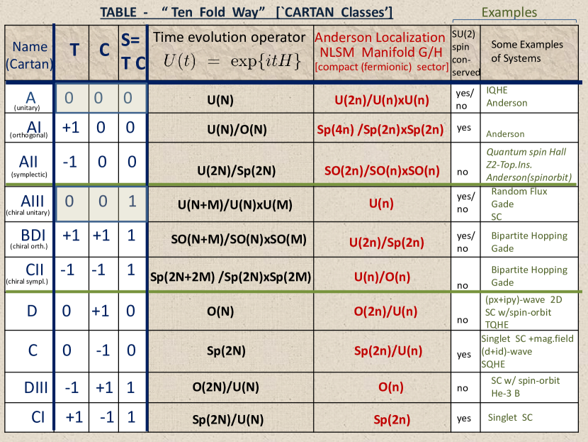
Figure 1: The “Ten-Fold Way”. Listed are the ten generic symmetry classes of first quantized Hamiltonians. This is a complete list of Hamiltonians which possess no unitarily realized symmetries. As reviewed in the text, the different symmetry classes can be characterized by their different behaviors of the first quantized Hamiltonian under time-reversal ($\bf T$), charge-conjugation ($\bf C$), and chiral symmetry (${\bf S}={\bf T}\cdot{\bf C}$). The column ‘Name (Cartan)’ lists the name given to the symmetric space appearing in the column ‘Time evolution operator’ by Élie Cartan in his classification scheme of symmetric spaces. The column ‘Anderson Localization NLSM Manifold G/H’ lists the (compact sectors of the) target space of the Non-Linear Sigma Model describing Anderson Localization physics in the corresponding symmetry class.

The column “Time evolution operator” of FIG. (1) shows what type of $N\times N$ matrix the first quantized time-evolution ${U}(t)=$ $\exp\{it{H}\}$ is. For example, the first row ("Cartan Symmetry Class A") lists systems with a Hamiltonian ${H}$ that possesses neither time-reversal (${T}=0$), nor charge-conjugation (${C}=0$), nor chiral symmetry (${S}=0$). There is no constraint on such a Hamiltonian, so it is a general hermitian $N\times N$ matrix (apart from conditions of locality). Therefore, the time-evolution operator is a general a unitary $N\times N$ matrix which is the meaning of the entry $U(N)$ in the first row of the Figure. To illustrate how to obtain the other entries in this column of the Figure, let us discuss the case of a Hamiltonian invariant under a (anti-unitary) time-reversal symmetry ${\bf T}$ which squares to plus the identity, ${\bf T}^{2}=+{\bf 1}$. This case is labeled by the "Cartan symbol" AI. We know that in this case there exists a basis in which the Hamiltonian is represented by a real symmetric matrix ${H}_{s}$. To understand the nature of the time-evolution operator in this case, let us first choose an arbitrary hermitean Hamiltonian ${H}$, and decompose it into symmetric and antisymmetric pieces, ${H}={1\over 2}({H}+{H}^{t})+{1\over 2}({H}-{H}^{t})$ $={H}_{s}+{H}_{a}$, where the superscript ^t denotes the transposed matrix. Hence, in a suitable basis, we can write the time-reversal symmetric Hamiltonian as ${H}_{s}={H}-{H}_{a}$; upon exponentiation, $\exp\{it{H}\}$ $={\rm unitary}$ $\in U(N)$, and $\exp\{it{H}_{a}\}=$ ${\rm orthogonal}$ $\in O(N)$. Therefore, the time-evolution operator of the time-reversal invariant system with ${\bf T}^{2}=+1$ is an element of the coset space $\exp\{it{H}_{s}\}$ $\in U(N)/O(N)$. This is the meaning of the entry in the 4th row of the Figure (with heading: "Time evolution operator"). The form of the time-evolution operator in all remaining eight cases can be determined analogously. What is interesting (and surprising) is that the result obtained for the list of ten time-evolution operators has a geometrical meaning. In the early parts of the last century, the mathematician Élie Cartan asked himself the following, seemingly completely unrelated question: What are all possible generalizations of spheres? (A sphere is an example of a space that has a constant curvature everywhere.) More precisely, can one write down a list of all possible Riemannian spaces (i.e. those that have a Riemannian metric) which have the same curvature everywhere (technically, where the Riemann curvature tensor is (covariantly) constant), and which have only a single curvature scale? Cartan found the answer in the year 1926: The list of ‘constant curvature spaces’ turns out to be precisely the set of ten (coset) spaces listed under the column “Time evolution operator” of FIG. (1) !

Let us now turn attention to the 6th column of FIG. (1) (with the heading “Anderson Localization NLSM Manifold G/H [compact (fermionic) sector]"). Note that the same set of 10 symmetric spaces appears as in the previous column (Time evolution operator), except that their order is permuted. In our context, this column refers to the $\overline{d}=$ $(d-1)$-dimensional boundary of the topological insulator in $d$ spatial bulk dimensions. A characteristic property of a non-interacting Fermion Topological Insulator is that while the bulk is insulating, there must always exist extended degees of freedom which are confined to the boundary, whose presence is protected by the topological nature of the bulk of the system. Physically, the presence of these extended degrees of freedom at the boundary implies that in contrast to the bulk, the boundaries conduct, depending on the case, electrical current or heat like a metal. (The existence of such extended (gapless) degrees of freedom on the boundary of the fully gapped bulk state may be viewed as an operational definition of the topological insulator.) These extended boundary degrees of freedom remain to be present when translational symmetry is broken, even if translational symmetry breaking is arbitrarily strong (but the corresponding energy scale is still well below the gap of the bulk state), because their existence is a consequence of the topological properties of the bulk, and translational symmetry (a unitarily implemented symmetry) is not necessary to protect the topological nature of the quantum state. The situation where translational invariance is broken (in practice often by the presence of impurities placed randomly within the sample, or due the presence of ‘random’ potentials, which typically result from the presence of such impurities) is commonly referred to as ‘disordered’ or ‘random’. The fact that these boundary degrees of freedom remain extended in the presence of translational symmetry breaking is very unusual because of the phenomenon of Anderson localizationAnderson (1958); Lee and Ramakrishnan (1985), which says that in ordinary systems (which are not boundaries of Topological Insulators or Superconductors) spatially extended eigenstates of the Hamiltonian become localized (i.e. exponentially decaying in space), at least for sufficiently strong breaking of translational symmetry (e.g. due the presence of ‘disorder’ potentials breaking translational symmetry). In practice the presence of extended eigenstates at the boundary of a topological insulator, even if translational symmetry is broken, implies that the boundary conducts electrical current or heat (similar to a metal), whereas the presence of only localized eigenstates would mean that the boundary is an electrical or thermal insulator. The boundaries of Topological Insulators (Superconductors) therefore always evade (“by definition") the phenomenon of Anderson localization. The theoretical description of Anderson localization phenomena is known to be very systematic and geometrical. For a Hamiltonian in one of the ten symmetry classes, the system (in the current situation the system in question is that at the boundary) is known to be described at length scales much larger than the ‘mean free path’ (which decribes the microscopic scale at which translational invariance is violated) by a Non-Linear Sigma Model (NLSM). A NLSM is a system like that describing the classical statistical mechanics of a Heisenberg ferromagnet. The only difference is that while for the Heisenberg ferromagnet a unit vector ‘spin’ is assigned to every point in space, which lives on a 2-dimensional unit sphere, in a general NLSM the unit vector ‘spin’ is replaced by an element of one of the ten Cartan symmetric spaces which, as we have mentioned, are all possible generalizations of spheres. These are listed in the 6th column of FIG. (1) with heading “Anderson Localization NLSM Manifold G/H [compact (fermionic) sector]". The general NLSM is decribed by a field theory whose (Boltzmann-type) weight is $\exp\{-S\}$ where

$$S={1\over g}\int d^{\overline{d}}r\ \sum_{\mu=1}^{\overline{d}}\ Tr\left(\partial_{\mu}\Phi(r)\partial_{\mu}\Phi(r)\right)$$ (34)

and the integral is over the $\overline{d}=$ $(d-1)$-dimensional boundary of the Topological Insulator in $d$ spatial dimensions. Here $\Phi(r)$ is a matrix field which is an element of the symmetric space G/H listed in the NLSM column of FIG. (1). [(The space G/H of which the ‘generalized Heisenberg spin’ $\Phi(r)$ is an element, is usually referred to as the ‘target space’, or the ‘target manifold’ of the NLSM. .)

We end by noting, as already mentioned at the beginning of section III, that a very interesting formulation of the Ten-Fold Way from a more mathematical perspective was recently developed in Freed and Moore (2013).

III.2 Classification by Topology of the Bulk: Translationally Invariant Case (K-Theory)

In this section we review how topology can be implemented in the general framework of the Ten-Fold-Way classification of Hamiltonians if we impose translational symmetry (so we can label all states by a momentum eigenvalue), and if we impose the condition that there is an excitation gap that separates all filled from all empty bands, so that the bulk is a "band insulator". In particular, in the presence of translational symmetry we can write the single-particle Hamiltonian $H$ in momentum space in the form

$$H(\vec{k})\ |u_{a}(\vec{k})\rangle\ =\ E_{a}(\vec{k})\ |u_{a}(\vec{k})\rangle$$ (35)

where ${\vec{k}}$ is the $d$-dimensional wavevector which is an element of the Brillouin zone (a torus). Here $a$ denotes the band index; we consider the case of $n$ filled and $m$ empty bands - see FIG. (2).

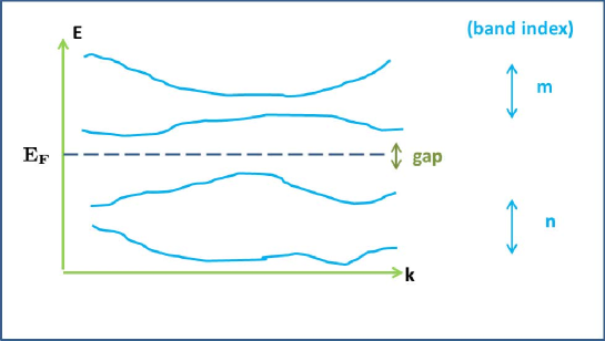
Figure 2: Typical band structure of a gapped band insulator. There are $n$ filled bands, and $m$ empty bands. $E_{F}$ denotes the Fermi energy.

Since we are interested in the topological properties of the system, we may continuously deform the Hamiltonian $H(\vec{k})$ to bring it into a simplified form where all filled bands have energy $E=-1$ and all empty band have energy $E=+1$ ("spectral flattening"). By definition, any topological properties will remain unchanged by such continuous deformations. We thereby obtain the "simplified Hamiltonian"

$${\mathbf{\cal\bf Q}}(\vec{k})={\rm Hamiltonian\ where}\ \ \ E_{a}(\vec{k})=\begin{cases}+1,&{\rm empty\ bands}\\ -1,&{\rm filled\ bands}.\end{cases}$$ (36)

III.2.1 Basic Ideas underlying the Classification and Simplest Example for Classification in the Bulk

In order to illustrate the idea of how to input information about topology, consider the simplest case of a Hamiltonian in a symmetry class that has no symmetry conditions at all. This is symmetry class $A$ in FIG. 1. Since the simplified Hamiltonian ${\mathbf{\cal\bf Q}}(\vec{k})$ has $n$ eigenvalues $E=-1$ and $m$ eigenvalues $E=+1$, it can be written in the form

$${\mathbf{\cal\bf Q}}(\vec{k})={\cal U}(\vec{k})\ \Lambda\ {\cal U}^{\dagger}(\vec{k}),\qquad{\rm where}\quad\Lambda=\left(\begin{matrix}{\bf 1}_{m}&{\bf 0}\\ {\bf 0}&{\bf-1}_{n}\end{matrix}\right),\quad{\rm and}\quad{\cal U}(\vec{k})\in U(m+n).$$ (37)

$\Lambda$ describes the eigenvalues, and ${\cal U}(\vec{k})\in U(m+n)$ describes the collection of all eigenvectors of ${\mathbf{\cal\bf Q}}(\vec{k})$. Now, when ${\cal U}(\vec{k})$ is of the form

$${\cal U}(\vec{k})=\left(\begin{matrix}U_{1}(\vec{k})&0\\ 0&U_{2}(\vec{k})\end{matrix}\right),\qquad{\rm where}\quad U_{1}(\vec{k})\in U(m)\quad{\rm and}\quad U_{2}(\vec{k})\in U(n),$$ (38)

${\mathbf{\cal\bf Q}}(\vec{k})$ remains unchanged from the value $=\Lambda$ that it takes when ${\cal U}(\vec{k})={\bf 1}_{m+n}$ . Therefore ${\mathbf{\cal\bf Q}}(\vec{k})$ only changes when ${\cal U}(\vec{k})$ is a non-trivial element of the coset space $G_{m,m+n}({\mathbf{C}})=$ $U(m+n)/[U(m)\times U(n)]$ which is conventionally called the (complex) "Grassmannian" $G_{m,m+n}({\mathbf{C}})$, i.e. when ${\cal U}(\vec{k})\in U(m+n)/[U(m)\times U(n)]$. Therefore we have established that every ground state of the simplified Hamiltonian ${\mathbf{\cal\bf Q}}(\vec{k})$ (where all $n$ bands are filled, and all $m$ bands are empty) is described by a map from the Brillouin zone (BZ) into the (complex) Grassmannian,

$${\mathbf{\cal\bf Q}}:BZ \rightarrow G_{m,m+n}({\mathbf{C}})=U(m+n)/[U(m)\times U(n)]$$ (39)

$${\vec{k}} \rightarrow {\mathbf{\cal\bf Q}}(\vec{k}).$$ (40)

Each such map describes a ground state, i.e. a filled Fermi sea of occupied states. Now, we want to know the answer to the question: How many different ground states of this kind, i.e. how many such different maps are there that cannot be continuously deformed into each other? For simplicity, let us assume that the Brillouin zone is a $d$-dimensional sphere (and not a $d$-dimensional torus, which it really is - we come back to the torus case shortly). In this case (i.e. for a $d$-dimensional "spherical" Brillouin zone) the answer is well known: It is given by the

$${Homotopy\ Group}\quad\pi_{d}\left(U(m+n)/[U(m)\times U(n)]\right)$$ (41)

which is known.

For example, when the spatial dimension is $d=2$, then it is known that $\pi_{d=2}\left(U(m+n)/[U(m)\times U(n)]\right)=$ ${\bf Z}$, the set of all integers. This means that for every integer there is a ground state, and ground states which are assigned different integers cannot be continuously deformed into each other (without closing the gap of the underlying bulk Hamiltonian $H(\vec{k})$). This particular result is of course not new, since the topological quantum state in $d=2$ spatial dimensions that appears for a single-particle Hamiltonian on which no symmetry conditions are imposed is the 2D integer quantum Hall state. The mentioned integer just counts the number of branches of chiral edge states, which tells us exactly which integer quantum Hall plateau the state describes.

Let us try the case of spatial dimension $d=3$, where $\pi_{d=3}\left(U(m+n)/[U(m)\times U(n)]\right)=$ $\{\bf 1\}$, i.e. the Homotopy Group is trivial and consists only of a single element. Therefore, our calculation predicts that in the present symmetry class (class A) there is only one state: All other states can be continously deformed into it. We have recovered the well known result that there are no integer quantum Hall states in $d=3$ spatial dimension.

III.2.2 General Classification in the Bulk - Results and K-Theory

Conceptually, the classification of Topological Insulators and Superconductors employing the current approach of determining the topology of the bulk states in the presence of translational invariance, proceeds analogously for all symmetry classes. In particular, for each of the 10 symmetry classes listed in FIG. 1, we need to find the corresponding "simplified Hamiltonian" ${\mathbf{\cal\bf Q}}(\vec{k})$. This task however turns out to be more complicated than that in (39) for symmetry class A, because the simplified Hamiltonian ${\cal\bf Q}(\vec{k})$ now has to reflect the invariance under the symmetries (time-reversal, charge-conjugation, chiral) which define the symmetry class. The corresponding list is displayed in TABLE 1.

Cartan Class	Simplified Hamiltonian
A	$\{\,{\cal\bf Q}(k)\in G_{m,m+n}(\mathbb{C})\,\}$
AI	$\{\,{\cal\bf Q}(k)\in G_{m,m+n}(\mathbb{C})\,|\,{\cal\bf Q}(k)^{*}={\cal\bf Q}(-k)\,\}$
AII	$\{\,{\cal\bf Q}(k)\in G_{2m,2(m+n)}(\mathbb{C})\,|\,({i}\sigma_{y}){\cal\bf Q}(k)^{*}(-{i}\sigma_{y})={\cal\bf Q}(-k)\,\}$
AIII	$\{\,{\bf q}(k)\in\mathrm{U}(m)\,\}$
BDI	$\{\,{\bf q}(k)\in\mathrm{U}(m)|{\bf q}(k)^{*}={\bf q}(-k)\,\}$
CII	$\{\,{\bf q}(k)\in\mathrm{U}(2m)\,|\,({i}\sigma_{y}){\bf q}(k)^{*}(-{i}\sigma_{y})={\bf q}(-k)\,\}$
D	$\{\,{\cal\bf Q}(k)\in G_{m,2m}(\mathbb{C})\,|\,\tau_{x}{\cal\bf Q}(k)^{*}\tau_{x}=-{\cal\bf Q}(-k)\,\}$
C	$\{\,{\cal\bf Q}(k)\in G_{m,2m}(\mathbb{C})\,|\,\tau_{y}{\cal\bf Q}(k)^{*}\tau_{y}=-{\cal\bf Q}(-k)\,\}$
DIII	$\{\,{\bf q}(k)\in\mathrm{U}(2m)\,|\,{\bf q}(k)^{T}=-{\bf q}(-k)\,\}$
CI	$\{\,{\bf q}(k)\in\mathrm{U}(m)\,|\,{\bf q}(k)^{T}={\bf q}(-k)\,\}$

Table 1: List of "simplified Hamiltonians" ${\mathbf{\cal\bf Q}}(\vec{k})$ for all ten symmetry classesSchnyder et al. (2008). As mentioned in the text, the (complex) Grassmannian is the coset space $G_{m,m+n}({\mathbf{C}})=U(m+n)/[U(m)\times U(n)]$. The meaning of the matrices ${\bf q}(k)$, which appear in all symmetry classes possessing chiral symmetry, is briefly explained in Appendix C.

The list of 10 "simplified Hamiltonians" displayed in TABLE 1 exhibits an interesting structure which is most easily revealed by looking at this list either in the special case of zero spatial dimensions, $d=0$, or in general spatial dimensions $d$ at special points ${\vec{k}}=$ ${\vec{k}}_{0}$ in the Brillouin zone which satisfy the property that $+{\vec{k}}_{0}$ and $-{\vec{k}}_{0}$ differ by a reciprocal lattice vector. The list of the corresponding "simplified Hamiltonian" matrices ${\mathbf{\cal\bf Q}}(\vec{k})$ is displayed in the rightmost column TABLE 2. Before commenting on this list, let us first elaborate on the subdivision of the 10 Cartan symmetry classes into "complex" and "real" ones. A look at FIG. 1 reveals that there are exactly two symmetry classes (classes A and AIII) which don’t possess any invariance under either of the two anti-unitary symmetries ${\bf T}$ or ${\bf C}$. All remaining eight symmetry classes are invariant under one or both of these anti-unitary symmetries: In particular, recall from (10) and (17) that each of the two anti-unitary symmetries imposes a reality condition on the Hamiltonian $H$. Thus we see that classes A and AIII are the only two classes in which no reality condition whatsoever is imposed on the Hamiltonian. It is for this reason that they are called "complex". On the other hand, in the remaining eight symmetry classes the Hamiltonian satisfies at least one reality condition. For this reason these symmetry classes are called "real". Now we come to the main point of TABLE 2: It reveals the remarkable observation that the simplified Hamiltonians ${\bf{\cal\bf Q}}(\vec{k})$ run again over the 10 symmetric spaces. But now these spaces appear yet in a different order as compared to the order in the column "Time evolution operator", and to the column "Anderson localization" in FIG. 1 .

Cartan	Time evolution operator			${\cal\bf Q}({\vec{k}})$
label	$\exp\{\mathrm{i}t{\cal H}\}$			Classifying Space
A	$\mathrm{U}(N)\times\mathrm{U}(N)/\mathrm{U}(N)$	("complex")		$\mathrm{U}(N+M)/\mathrm{U}(N)\times\mathrm{U}(M)$	$=C_{0}$
AIII	$\mathrm{U}(N+M)/\mathrm{U}(N)\times\mathrm{U}(M)$			$\mathrm{U}(N)\times\mathrm{U}(N)/\mathrm{U}(N)$	$=C_{1}$
AI	$\mathrm{U}(N)/\mathrm{O}(N)$			$\mathrm{O}(N+M)/\mathrm{O}(N)\times\mathrm{O}(M)$	$=R_{0}$
BDI	$\mathrm{O}(N+M)/\mathrm{O}(N)\times\mathrm{O}(M)$			$\mathrm{O}(N)\times\mathrm{O}(N)/\mathrm{O}(N)$	$=R_{1}$
D	$\mathrm{O}(N)\times\mathrm{O}(N)/\mathrm{O}(N)$			$\mathrm{O}(2N)/\mathrm{U}(N)$	$=R_{2}$
DIII	$\mathrm{SO}(2N)/\mathrm{U}(N)$	("real")		$\mathrm{U}(2N)/\mathrm{Sp}(2N)$	$=R_{3}$
AII	$\mathrm{U}(2N)/\mathrm{Sp}(2N)$			$\mathrm{Sp}(N+M)/\mathrm{Sp}(N)\times\mathrm{Sp}(M)$	$=R_{4}$
CII	$\mathrm{Sp}(N+M)/\mathrm{Sp}(N)\times\mathrm{Sp}(M)$			$\mathrm{Sp}(N)\times\mathrm{Sp}(N)/\mathrm{Sp}(N)$	$=R_{5}$
C	$\mathrm{Sp}(2N)\times\mathrm{Sp}(2N)/\mathrm{Sp}(2N)$			$\mathrm{Sp}(2N)/\mathrm{U}(N)$	$=R_{6}$
CI	$\mathrm{Sp}(2N)/\mathrm{U}(N)$			$\mathrm{U}(N)/\mathrm{O}(N)$	$=R_{7}$

Table 2: ListRyu et al. (2010) of time-evolution operators and "simplified Hamiltonians" ${\mathbf{\cal\bf Q}}(\vec{k})$ in either zero spatial dimension, or in arbitrary spatial dimensions at special points ${\vec{k}}=$ ${\vec{k}}_{0}$ in the Brillouin zone which satisfy the property that $+{\vec{k}}_{0}$ asnd $-{\vec{k}}_{0}$ differ by a reciprocal lattice vector. The sets of "simplified Hamiltonians" ${\mathbf{\cal\bf Q}}(\vec{k})$ listed in the rightmost column are the so-called "Classifying Spaces" of K-Theory. They are called $C_{0}$ and $C_{1}$ for the complex symmetry classes, and $R_{q}$ with $q=0,1,2,...,7$ (modulo 8) in the real symmetry classes. The Classifying Spaces run again over all symmetric spaces, but in an order that is different from that enountered in the column "Time evolution operator". Note that in the left column "Time evolution operator" the numbers $N$ and $M$ physically denote numbers of lattice sites. In the right column "Classifying space" the $N$ and $M$ denote the numbers of filled and empty bands, generalizing the setup in FIG. 2.

At this point is it basically clear conceptually how to go about the classification in the bulk. We have to repeat the analysis of section III.2.1 for all the remaining nine "simplified Hamiltonians" ${\bf{\cal\bf Q}}(\vec{k})$ listed in TABLE 1. It turns out that this is a rather involved task, due to constrains arising from the three symmetry operations defining the ten symmetry classes. However, it turns out that K-Theory is the tool that precisely answers this question. While we will not review here the apparatus of K-Theory, it is easy to state the result and explain the physical features appearing in it. Let us list the result for the real symmetry classes. They are denoted by the symbols $R_{q}$ which are defined in the rightmost column of TABLE 2. The result due to Kitaev readsKitaev (2009)

$$\pi\left(\overline{{\rm T}^{d}},R_{q}\right)\ \ =\ \ \pi_{0}\left(R_{q-d}\right)\ \ \oplus\ \ \bigoplus_{s=0}^{d-1}\ \ \left(\begin{matrix}d\\ s\end{matrix}\right)\ \ \pi_{0}\left(R_{q-s}\right).$$ (42)

The symbol $\pi\left(\overline{{\rm T}^{d}},R_{q}\right)$ appearing on the left hand side of the above equation generalizes the Homotopy Groups appearing in (41). The generalization is twofold. The above symbol generalizes (i) the Homotopy Group to maps from the actual d-dimensional Brillouin zone torus (hence the appearance of $T^{d}$) and not from the d-dimensional "spherical Brillouin zone", and (ii) to all the eight real symmetry classes which are labeled by the symbold $R_{q}$, defined in TABLE 2, taking into account all the constraints listed in TABLE 1 (hence the "bar" over $T^{d}$). The result on the right hand side of (42) contains nothing but the zeroth Homotopy Groups of the various Classifying spaces $R_{q}$. (These are known and will be listed explicitly in subsequent Tables or Figures.) The result on the right hand side of (42) consists of two pieces, the first piece "$\pi_{0}\left(R_{q-d}\right)$" and remaining sum "$\bigoplus_{s=0}^{d-1}\left(\begin{matrix}d\\ s\end{matrix}\right)\ \ \pi_{0}\left(R_{q-s}\right)$" . The first piece turns out to be the universal piece of interest to us, which is not tied to the presence of translational invariance. If this first piece is non-trivial we have what is called a "strong Topological Insulator or Superconductor", whose topological properties would persist even if translational symmetry was broken. On the other hand it is clearly seen already from the structure of the second piece that it relies on the presence of translational order: The various $d$ terms in the summand of the second piece describe the presence or absence of a Topological Insulator or Superconductor phase on submanifolds of dimension $s=$ $(d-1),(d-2),...,0$. In particular, the term with $s=(d-1)$ describes the presence or absence of a Topological Insulator (Superconductor) in hyperplanes of the $d$-dimensional lattice (of codimension $=1$), $s=(d-2)$ describes submanifolds of the lattice of condimension $=2$ (e.g. one lines in a $d=3$ dimensional lattice), etc.. The term $s=0$ describes such toplogical properties associated with points. The factor $\left({}^{d}_{s}\right)$ counts the number of ways the $s$-dimensional objects can be placed into the $d$-dimensional lattice. None of these lower dimensional objects would be defined in the absence of the lattice. For this reason the second piece characterizes "weak Topological Insulators (Superconductors)" which can exist in the system. Finally, there is a corresponding expression for the two complex symmetry classes A and AIII, and the corresponding complex Classifying Spaces called $C_{q}$, $q=0,1$. By keeping only the first, universal piece on the right hand side of (42) as well as the corresponding "complex" version, one arrives at the Table of Topological Insulators and Superconductors displayed in TABLE 3.

We end by noting that, as already mentioned at the beginning of section III, a somewhat different approach to topological band theory, which does not use K-Theory, was very recently developed in Kennedy and Zirnbauer (2014a) (see also the contribution Kennedy and Zirnbauer (2014b) to the present Nobel Symposium).

Cartan$\backslash d$	0	1	2	3	4	5	6	7	8
Complex case:
A	$\mathbb{Z}$	0	$\mathbb{Z}$	0	$\mathbb{Z}$	0	$\mathbb{Z}$	0	$\mathbb{Z}$  $\cdots$
AIII	0	$\mathbb{Z}$	0	$\mathbb{Z}$	0	$\mathbb{Z}$	0	$\mathbb{Z}$	0  $\cdots$
Real case:
AI	$\mathbb{Z}$	0	0	0	$2\mathbb{Z}$	0	$\mathbb{Z}_{2}$	$\mathbb{Z}_{2}$	$\mathbb{Z}$  $\cdots$
BDI	$\mathbb{Z}_{2}$	$\mathbb{Z}$	0	0	0	$2\mathbb{Z}$	0	$\mathbb{Z}_{2}$	$\mathbb{Z}_{2}$  $\cdots$
D	$\mathbb{Z}_{2}$	$\mathbb{Z}_{2}$	$\mathbb{Z}$	0	0	0	$2\mathbb{Z}$	0	$\mathbb{Z}_{2}$  $\cdots$
DIII	0	$\mathbb{Z}_{2}$	$\mathbb{Z}_{2}$	$\mathbb{Z}$	0	0	0	$2\mathbb{Z}$	0  $\cdots$
AII	$2\mathbb{Z}$	0	$\mathbb{Z}_{2}$	$\mathbb{Z}_{2}$	$\mathbb{Z}$	0	0	0	$2\mathbb{Z}$  $\cdots$
CII	0	$2\mathbb{Z}$	0	$\mathbb{Z}_{2}$	$\mathbb{Z}_{2}$	$\mathbb{Z}$	0	0	0  $\cdots$
C	0	0	$2\mathbb{Z}$	0	$\mathbb{Z}_{2}$	$\mathbb{Z}_{2}$	$\mathbb{Z}$	0	0  $\cdots$
CI	0	0	0	$2\mathbb{Z}$	0	$\mathbb{Z}_{2}$	$\mathbb{Z}_{2}$	$\mathbb{Z}$	0  $\cdots$

Table 3: Table of Topological Insulators and SuperconductorsSchnyder et al. (2008, 2009); Kitaev (2009); Ryu et al. (2010) .

III.3 Classification by Lack of Anderson Localization on the Boundary (Non-Linear Sigma Models)

The technically simplest way to obtain the Table of Topological Insulators and Superconductors, TABLE 3, is to focus on the classification of boundaries of the system, as opposed to the approach in the previous section III.2 which focused on the bulk. The characterization of Topological Phases in terms of their boundaries has proven more generally to be one of the most successful tools in this subject area. This is related to the fact that these boundaries must exhibit an "anomaly" of some kind, a fact that was first recognized in its general form in the context of non-interacting Fermionic Topological Insulators and Superconductors in Ryu et al. (2012), and this is discussed in section III.5 below. The characterization of more general Topological Phases, including interacting systems, by anomalies at their boundaries has become a key tool in this area. (See also the comments in sections II and III.5.) In the case of non-interacting Fermionic Topological Insulators (Superconductors) the anomalous properties of the sample boundaries manifest themselves through the fact that the boundaries must always possess extended states. This means that the boundaries always conduct electrical current or heat similar to a metal. Because of the well known phenomenon of Anderson localization this provides a very convenient and quick way to classify Toplogical Insulators (Superconductors), as we will now review.

As already mentioned above, Anderson localization is the phenomenon that, at least for sufficiently strong breaking of translational invariance (typically introduced by potentials that arise from randomly located impurities - "disorder"), spatially extended eigenstates of the Hamiltonian $H$ tend to become localized in space (typically exponentially decaying in space about a point)Anderson (1958); Lee and Ramakrishnan (1985). The resulting phase is the so-called Anderson Insulator which, hence, typically always occurs at least for sufficiently strong breaking of translational invariance. Now, the point is that the Anderson Insulator is a phase that does not conduct electrical current nor heat, and therefore is not allowed to occur at the boundaries of a Topological Insulator or Superconductor. Thus, the boundary of any Topological Insulator or Superconductor must entirely evade the phenomeon of Anderson Localization. As we will now see, this condition can be fairly easily exploited at the technical level, and this directly yields the classification of Topological Insulators (Superconductors), TABLE 3.

In summary, the current method of classification amounts to the following: We reduce the problem of classifying Topological Insulators (Superconductors) in $d$ spatial dimensions to a problem of Anderson Localization in $\overline{d}=$ $(d-1)$ dimensions (i.e. "at the boundary"). By studying the lack of Anderson Localization in $\overline{d}=$ $(d-1)$ spatial dimensions, we solve the classification problem of Topological Insulator (Superconductors) in $d$ spatial dimensions.

In order to understand how to implement this program in practice, all one needs to appreciate is that the answer to the question about the lack of Anderson Localization is a question in Field Theory. It is well known that the theoretical description of problems of Anderson Localization is very systematic and geometrical (See e.g. Efetov (1997); Wegner (1979); Zirnbauer (1996)). Microscopically, the underlying first quantized Hamiltonian $H$ is a member of one of the ten symmetry classes, FIG. 1, in every realization of disorder. Physically, this is in our current discussion the Hamiltonian describing the $\overline{d}=$ $(d-1)$ dimensional boundary of the $d$-dimensional Topological Insulator (Superconductor) in question which will lie in the same symmetry class as the bulk. It turns out that at long length scales (i.e. at scales much larger than the "mean free path", the corresponding small length scale in this kind of problem) a description in terms of a Non-Linear Sigma Model (NLSM) field theory emerges. As already briefly mentioned above, a general NLSM is a simple generalization of the theory we use in standard Statistical Mechanics to describe the classical Heisenberg Ferromagnet. The Ferromagnet can be formulated as a model of a unit vector spin, at every point in space, that points to the surface of a two-dimensional sphere (in three dimensional spin space). The energy is simply a gradient square of such a spin configuation. A general NLSM of interest in the present context is the same type of theory, except that the field, the unit vector spin that used to represent an element of a sphere in the Ferromagnet, is now replaced by an element of one of the ten symmetric spaces listed in the 6th column of FIG.1 (with the heading "Anderson Localization, NLSM Manifold G/H"). As mentioned towards the end of Section III.1.3, the ten symmetric spaces $G/H$ appearing in FIG.1 are generalizations of spheres (according to the seminal work by the mathematician Élie Cartan). The general NLSM is therefore described by a "Boltzmann"-type weight (‘action’) of the form already displayed in (34), where the coupling constant $g$ changes with the amount of translational symmetry breaking ("disorder"). NLSMs of the form (34) will always possess an Anderson Insulator phase, at least for sufficiently large values of the coupling constant $g$. In the Anderson Insulator phase the correlation length is finite. At the boundary of a Topological Insulator (Superconductor), the corresponding NLSM must however always describe a (electrical or heat) conductor, which means that the correlation length must be infinite. Now, the NLSM on the $\overline{d}$ dimensional boundary completely evades the phenomenon of Anderson Localization if a certain extra term of topological origin with no adjustable parameter can be added to the action (34) of the NLSM:

$$S={1\over g}\int d^{\overline{d}}r\ \sum_{\mu=1}^{\overline{d}}\ Tr\left(\partial_{\mu}\Phi(r)\partial_{\mu}\Phi(r)\right)+S_{top}\{\Phi(r)\},\qquad\Phi(r)\in G/H={\rm"target\ space"}.$$ (43)

The question whether a suitable such term of topological origin $S_{top}$ exists or not, depends (i) on the "target space" $G/H$ of the NLSM which is determined by the symmetry class of the underlying Topological Insulator (Superconductor) in $d$ spatial dimension, as determined by FIG.1, and (ii) on the dimension $\overline{d}=$ $(d-1)$ of the boundary on which the NLSM is defined. There is however a simple answer to this question: It is the Homotopy Group of the target space $G/H$ which determines whether a suitable term exists. Namely, the target space $G/H$ of the NLSM allows for

$$(a) :\quad{\rm a}\ Z_{2}\ {\rm topological\ term}\qquad\qquad\qquad\ \ \ {\rm\it if\ and\ only\ if}\qquad\pi_{\overline{d}}\left(G/H\right)=\pi_{d-1}\left(G/H\right)={\mathbf{Z}_{2}}$$ (44)

$$(b) :\quad{\rm a\ {Wess-Zumino-Witten}\ term}\ \qquad{\rm\it if\ and\ only\ if}\qquad\pi_{\overline{d}+1}\left(G/H\right)=\pi_{d}\left(G/H\right)={\bf Z}.$$ (45)

We will now implement this rule to determine the list of Topological Insulators (Superconductors). To this end, we display in FIG. 3 a Table containing the list of the Homotopy Groups $\pi_{s}\left(G/H\right)$ for all 10 symmetric spaces $G/H$. The left-arrows indicate that due to (45) the boundary dimension $\overline{d}$ of the Topological Insulator (Superconductor) with the corresponding ${\bf Z}$ classification is located at the position to which the end of the arrow points. After moving all entries ${\bf Z}$ to the end of the corresponding arrows, and after shifting all columns of the Table in FIG. 3 (i.e. $\overline{d}\to$ $d=\overline{d}+1$) - this implements the rules specified in (44, 45) - one obtains from FIG. 3 directly the Table of Topological Insulators and Superconductors, TABLE 4 (which is a copy of TABLE 3, reproduced again for the convenience of the reader).

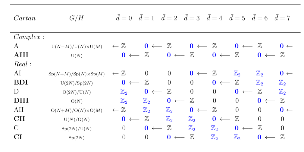
Figure 3: Table of Homotopy Groups $\pi_{s}\left(G/H\right)$ of the ten symmetric spaces appearing in the Ten-Fold-Way.Lundell (1992); Ryu et al. (2010). Here, according to (44), $s=\overline{d}$ when $\pi_{s}\left(G/H\right)=$ ${\bf Z_{2}}$, whereas according to (45), $s=\overline{d}+1$ when $\pi_{s}\left(G/H\right)=$ ${\bf Z}$. The left-arrows indicate that due to (45) the boundary dimension $\overline{d}$ of the Topological Insulator (Superconductor) with the corresponding ${\bf Z}$ classification is located at the end of the arrow. After moving all entries ${\bf Z}$ to the end of the corresponding arrows, and after shifting all columns of the Table in FIG. 3 - this implements the rules specified in (44, 45) - one obtains from FIG. 3 directly the Table of Topological Insulators and Superconductors, TABLEs 3 and 4.

Cartan$\backslash d$	0	1	2	3	4	5	6	7	8
Complex case:
A	$\mathbb{Z}$	0	$\mathbb{Z}$	0	$\mathbb{Z}$	0	$\mathbb{Z}$	0	$\mathbb{Z}$  $\cdots$
AIII	0	$\mathbb{Z}$	0	$\mathbb{Z}$	0	$\mathbb{Z}$	0	$\mathbb{Z}$	0  $\cdots$
Real case:
AI	$\mathbb{Z}$	0	0	0	$2\mathbb{Z}$	0	$\mathbb{Z}_{2}$	$\mathbb{Z}_{2}$	$\mathbb{Z}$  $\cdots$
BDI	$\mathbb{Z}_{2}$	$\mathbb{Z}$	0	0	0	$2\mathbb{Z}$	0	$\mathbb{Z}_{2}$	$\mathbb{Z}_{2}$  $\cdots$
D	$\mathbb{Z}_{2}$	$\mathbb{Z}_{2}$	$\mathbb{Z}$	0	0	0	$2\mathbb{Z}$	0	$\mathbb{Z}_{2}$  $\cdots$
DIII	0	$\mathbb{Z}_{2}$	$\mathbb{Z}_{2}$	$\mathbb{Z}$	0	0	0	$2\mathbb{Z}$	0  $\cdots$
AII	$2\mathbb{Z}$	0	$\mathbb{Z}_{2}$	$\mathbb{Z}_{2}$	$\mathbb{Z}$	0	0	0	$2\mathbb{Z}$  $\cdots$
CII	0	$2\mathbb{Z}$	0	$\mathbb{Z}_{2}$	$\mathbb{Z}_{2}$	$\mathbb{Z}$	0	0	0  $\cdots$
C	0	0	$2\mathbb{Z}$	0	$\mathbb{Z}_{2}$	$\mathbb{Z}_{2}$	$\mathbb{Z}$	0	0  $\cdots$
CI	0	0	0	$2\mathbb{Z}$	0	$\mathbb{Z}_{2}$	$\mathbb{Z}_{2}$	$\mathbb{Z}$	0  $\cdots$

Table 4: Table of Topological Insulators and SuperconductorsSchnyder et al. (2008, 2009); Kitaev (2009); Ryu et al. (2010) .

III.4 Mathematical Reason for Agreement between Bulk- and Boundary- based Classifications

While the bulk-based classification method from section III.2, based on an analysis of topological band theory, and the boundary-based classification from section III.3, based on the lack of Anderson Localization on the boundary, must yield the same result on physical grounds (as they do), it is a priori not clear what the technical (i.e. mathematical) reason for this agreement is, since the two methods appear to be based on conditions that look mathematically very different. By explicitly comparing these two conditions, we will now exhibit a certain "symmetry" property inherent in Table of Homotopy Groups, FIG. 3, that is responsible for the agreement of the two methods.

			$R_{4-p}$		$R_{p}$
			$\Downarrow$		$\Downarrow$
Cartan	Time evolution operator	Fermionic replica		Classifying
label	$\exp\{\mathrm{i}t{\cal H}\}$	NLSM target space		space
A	$\mathrm{U}(N)\times\mathrm{U}(N)/\mathrm{U}(N)$	$\mathrm{U}(2n)/\mathrm{U}(n)\times\mathrm{U}(n)$	$=C_{0}$	$\mathrm{U}(N+M)/\mathrm{U}(N)\times\mathrm{U}(M)$	$=C_{0}$
AIII	$\mathrm{U}(N+M)/\mathrm{U}(N)\times\mathrm{U}(M)$	$\mathrm{U}(n)\times\mathrm{U}(n)/\mathrm{U}(n)$	$=C_{1}$	$\mathrm{U}(N)\times\mathrm{U}(N)/\mathrm{U}(N)$	$=C_{1}$
AI	$\mathrm{U}(N)/\mathrm{O}(N)$	$\mathrm{Sp}(2n)/\mathrm{Sp}(n)\times\mathrm{Sp}(n)$	$=R_{4}$	$\mathrm{O}(N+M)/\mathrm{O}(N)\times\mathrm{O}(M)$	$=R_{0}$
BDI	$\mathrm{O}(N+M)/\mathrm{O}(N)\times\mathrm{O}(M)$	$\mathrm{U}(2n)/\mathrm{Sp}(2n)$	$=R_{3}$	$\mathrm{O}(N)\times\mathrm{O}(N)/\mathrm{O}(N)$	$=R_{1}$
D	$\mathrm{O}(N)\times\mathrm{O}(N)/\mathrm{O}(N)$	$\mathrm{O}(2n)/\mathrm{U}(n)$	$=R_{2}$	$\mathrm{O}(2N)/\mathrm{U}(N)$	$=R_{2}$
DIII	$\mathrm{SO}(2N)/\mathrm{U}(N)$	$\mathrm{O}(n)\times\mathrm{O}(n)/\mathrm{O}(n)$	$=R_{1}$	$\mathrm{U}(2N)/\mathrm{Sp}(2N)$	$=R_{3}$
AII	$\mathrm{U}(2N)/\mathrm{Sp}(2N)$	$\mathrm{O}(2n)/\mathrm{O}(n)\times\mathrm{O}(n)$	$=R_{0}$	$\mathrm{Sp}(N+M)/\mathrm{Sp}(N)\times\mathrm{Sp}(M)$	$=R_{4}$
CII	$\mathrm{Sp}(N+M)/\mathrm{Sp}(N)\times\mathrm{Sp}(M)$	$\mathrm{U}(n)/\mathrm{O}(n)$	$=R_{7}$	$\mathrm{Sp}(N)\times\mathrm{Sp}(N)/\mathrm{Sp}(N)$	$=R_{5}$
C	$\mathrm{Sp}(2N)\times\mathrm{Sp}(2N)/\mathrm{Sp}(2N)$	$\mathrm{Sp}(2n)/\mathrm{U}(n)$	$=R_{6}$	$\mathrm{Sp}(2N)/\mathrm{U}(N)$	$=R_{6}$
CI	$\mathrm{Sp}(2N)/\mathrm{U}(N)$	$\mathrm{Sp}(2n)\times\mathrm{Sp}(2n)/\mathrm{Sp}(2n)$	$=R_{5}$	$\mathrm{U}(N)/\mathrm{O}(N)$	$=R_{7}$

Table 5: ComparisonRyu et al. (2010) of the order of the three occurrences of the 10 Cartan Symmetric Spaces. (Symmetry Classes with Chiral Symmetry are marked in bold face). For the eight real cases, the last column ("Classifying space") lists the spaces $R_{p}$ where $p=0,1,...,7$ $({\rm mod}\ 8)$ in ascending order downwards, whereas the corresponding symmetric space in the middle column ("Fermionic replica NL$\sigma$M target space") is seen to be $R_{4-p}$. - As also seen from the TABLE, the corresponding symmetric space in the column "Time evolution operator" is $R_{p-1}$ as compared to the last column. The corresponding shift $C_{0}\leftrightarrow$ $C_{1}$ for the two complex symmetric spaces $C_{0}$ and $C_{1}$ is also clearly visible.

To this end, it is useful to compare the three different occurrences of the 10 Cartan Symmetric Spaces in the classification. This can be seen from TABLE 5: Let us first focus on the eight real classes, which are listed in descending order in the 4th (last) column of this TABLE, and are denoted by $R_{p}$ $(p=0,1,...,7$ (mod $8$). The 3rd column of the TABLE, with the heading "Fermionic replica NLSM target spaces", lists the NLSM target spaces $G/H$ of Anderson Localization, which appear in the permutation $R_{4-p}$ $\Leftrightarrow$ $R_{p}$ as compared to the 4th column, as also indicated in the TABLE. (We also see that the corresponding symmetric space in the 2nd column with the heading "Time evolution operator" is $R_{p-1}$.) Now, the conditions (44, 45) for obtaining a Topological Insulator (Superconductor) based on the Boundary method (Anderson Localization - NLSM) are displayed on the right hand sides of (46). Here we used the property $\ \pi_{d}\left(R_{p}\right)=\pi_{0}\left(R_{p+d}\right)$ which can immediately be read off from the Table of Homotopy Groups, FIG. 3. On the other hand, the conditions (42) based on the Bulk method (Topology of Bulk Band Structure) are displayed on the left hand sides of (46). As mentioned above, it is not immediately obvious that the conditions arising from the "Bulk" and "Boundary" methods are the same. However, it is not difficult to check using FIG.3 that these conditions are indeed the same, which is a certain built-in "symmetry" property of the Table of Homotopy Groups, FIG.3. (Details are provided in Appendix (D).)

$$\left\{\begin{matrix}{\rm\bf\underline{\bf Bulk:}\ Topological\ Band\ Theory}&&{\rm\bf\underline{\bf Boundary:}\ Anderson\ Localization(NLSM)}\\ &&\\ (a):\qquad\qquad{\color[rgb]{0,0,1}\pi_{0}\left(R_{q-d}\right)={\bf Z_{2}}}\qquad&{\rm\it if\ and\ only\ if}&\left[\pi_{d-1}\left(R_{4-q}\right)=\right]\ \ {\color[rgb]{0,0,1}\pi_{0}\left(R_{3-(q-d)}\right)={\bf Z_{2}}}\\ (b):\qquad\qquad{\color[rgb]{1,0,0}\pi_{0}\left(R_{q-d}\right)={\bf Z}}\ \qquad&{\rm\it if\ and\ only\ if}&\ \ \left[\pi_{d}\left(R_{4-q}\right)=\right]\ \ {\color[rgb]{1,0,0}\pi_{0}\left(R_{4-(q-d)}\right)={\bf Z}}\\ &&\\ &{\rm using:}\ \pi_{d}\left(R_{p}\right)=\pi_{0}\left(R_{p+d}\right)&\end{matrix}\right\}$$ (46)

III.5 Perspective of Quantum Anomalies

As already mentioned at the beginning of section III, a third classifying principle has emerged, besides those discussed in sections III.2 and III.3. This new classifying principle, which is based on Quantum Anomalies that are forced to occur at the boundary of Topological Insulators and Superconductors, is probably the most general such principle as it will extend also to interacting theories; it has been the topic of much recent discussions. (For a very short (and incomplete) list of references to recent discussions see e.g. Sule et al. (2013); Ryu (2015); Wang and Senthil (2014); Kapustin et al. (2014); Witten (2015).) This principle was first recognized in Ref. Ryu et al. (2012) in its general form in the context of non-interacting Fermionic Topological Insulators and Superconductors. The perspective of Quantum Anomalies of Topological Insulators (Superconductors) can be viewed as a generalization of the boundary-based classification principle invoking Anderson Localization that was reviewed in section III.3. It relies on the notion that the boundary of a Topological Insulator (Superconductor) cannot exist as an isolated system in its own dimensionality. Rather it must always be attached to a higher dimensional bulk. Technically, the inability of the boundary of the system to exist in isolation is rooted in certain ill-defined properties the boundary would possess in isolation. It was in Ref. Ryu et al. (2012) that such ill-defined properties of the boundary of non-interacting Fermionic Topological Insulators (Superconductors) were in general related to the notion of Quantum Anomalies known from work in the 1980ies in relativistic Quantum Field Field Theory and Elementary Particle Physics (see e.g. Alvarez-Gaumé and Witten (1983); Alvarez-Gaumé and Ginsparg (1985)). We will review the basic ideas of Ryu et al. (2012) in this section.

In general, a quantum system possesses a Quantum Anomaly if the corresponding classical system is invariant under some (global or gauge) symmetry, and this symmetry gets lost in the process of quantization. For technical reasons it is useful to take advantage of the following result that emerged from the classification of Topological Insulators and Superconductors: It turns out that every Topological Insulator (Superconductor) phase of non-interacting Fermions, in any dimension, has a massive Dirac Hamiltonian representative in the same topological classRyu et al. (2010); Kitaev (2009); Teo and Kane (2010). Since we are only interested in the topological properties of the phase, we are free to consider the Dirac Hamiltonian representative. Next, we couple the Dirac Hamiltonian representative to suitable space and time dependent classical background fields. These could be a $U(1)$-gauge field if the Topological Insulator (Superconductor) has a conserved $U(1)$ charge, an $SU(2)$-gauge field if it has $SU(2)$ symmetry, etc.. If, on the other hand, we have a Topological Superconductor which is not invariant under any continuous symmetries (examples are known in Cartan Symmetry Classes D and DIII), then we can still couple the Dirac Hamiltonian to a background gravitational field, i.e. we put it in a curved background. In either case we end up, after integrating out the gapped Fermions, with an effective action for the classical space and time dependent background fields (in the gravitational case, the effective action depends on the background metric). For example in the case of a $U(1)$ background gauge field $A_{\mu}(x)$ we obtain an effective action

$$e^{-W_{eff}[A_{\mu}]}\ \equiv \ \int{\cal D}[{\bar{\psi}},\psi]\ e^{-S[{\bar{\psi}},\psi;A_{\mu}]}.$$ (47)

We work in imaginary time where $x$ denotes the $D=d+1$ space-time coordinates $x=(\tau,{\vec{x}})$, and ${\vec{x}}$ the spatial coordinates. As indicated in the second line of the above equation, the effective action for the gauge field, which physically describes the responses of the system to the external classical perturbation $A_{\mu}$, can have, besides a possible "standard" or "usual" term (in $D=4$ space-time dimensions and in the case of a $U(1)$ gauge field this will be Maxwell action for electromagnetism in the medium of the Topological Insulator (Superconductor)), an unusual or anomalous response arising from a topological term $W_{top}$. That latter (anomalous) response would never exist for an "ordinary" system describing a boundary that is allowed to exist in isolation without an attached bulk. It only occurs for boundaries of Topological Insulators (Superconductors).

It turns out that in general we need to distinguish two types of such anomalous responses which will be defined in more detail below: (i) Chern-Simons type responses, occuring in odd space-time dimensions $D=d+1=$ $2n-1$, and (ii) Theta term type responses, occuring in even space-time dimensions $D=d+1=$ $2n$. In the following section we will describe two well-known special cases of these anomalous responses in $D=3$ and $D=4$ space-time dimensions. In the subsequent section, we will generalize them and show how to use the so-obtained generalized responses to predict various Topological Insulators and Superconductors occuring in TABLE 3 .

III.5.1 Examples: Chern-Simons term in Integer Quantum Hall effect in $D=3$ space-time dimensions, and Theta Term in standard ${\bf Z_{2}}$ Topological Insulator in $D=4$ space-time dimensions.

(i) Chern-Simons type response: $d=2$ ($D=3$) Integer Quantum Hall effect. Let us consider an (spatial) annulus filled with the Integer Quantum Hall state - marked red in FIG. 4. There are two counterpropagating chiral edge modes at the boundaries of the annulus. Let us consider the theory describing one of these boundaries in $D=2=(1+1)$ dimensional space-time. We know that charge conservation at such a boundary is spoiled by quantum effects: charge will ‘leak’ from the boundary into the bulk (the annulus) and eventually to the other boundary. The $d=2$ Integer Quantum Hall state is in Cartan Symmetry Class $A$, and is thus one of the Topological Insulators in the 10-fold Table. The ‘leaking’ of charge indicates that the bounday cannot exist in isolation but must be the boundary of a Topological Insulator in one dimension higher.

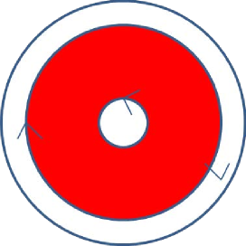
Figure 4: Annulus Geometry for the Quantum Hall Effect. In the present discussion we consider only the case of the Integer Quantum Hall effect.

How is this seen from the perspective of the bulk? As is well known, the topological part of the action defined in (47) is in the present case a (Abelian) Chern-Simons term

$$W_{top}=i\sigma_{xy}\int d^{2}{\vec{x}}d\tau\ {(-1)\over 4\pi}\epsilon^{\mu\nu\lambda}A_{\mu}\partial_{\nu}A_{\lambda},\qquad{\rm where}\quad\sigma_{xy}={\rm integer}.$$ (48)

(Here $\sigma_{xy}$ is the Hall conductivity measured in units of $e^{2}/h$.) As we will discuss in more detail for the general cases, a Chern-Simons term defined on a space-time manifold with boundaries is not invariant under gauge transformations performed on the gauge field $A_{\mu}$. It is this lack of gauge invariance of the bulk that will have to be compensated for by the theory describing the boundary, so that the combined system is gauge invariant (as it is). So the appearance of the Chern-Simons term $W_{top}$ of the $D=3$ dimensional bulk indicates that there is anomaly at the boundary, and it allows us to identify and quantify this anomaly of the theory describing the boundary. As we will discuss in the next section, various generalized versions of Chern-Simons terms will occur in all odd space-time dimensions.

(ii) Theta-term type response: $d=3$ ($D=4$) ${\bf Z_{2}}$ Topological Insulator. Let us consider the "standard" ${\bf Z_{2}}$ Topological Insulator in Cartan Symmetry Class AII in $d=3$ spatial dimensions (see e.g. Hasan and Kane (2010)). It was first observed in Qi et al. (2008) that after minimally coupling to a $U(1)$ gauge field $A_{\mu}$ the effective action for the gauge field contains, besides the usual Maxwell term, a topological term which is an example of a class of topological terms that are in general called $\theta$-terms,

$$W_{top} = i\theta\int_{{\cal M}_{4}}{(-1)\over 32\pi^{2}}\epsilon^{\mu\nu\kappa\lambda}F_{\mu\nu}F_{\kappa\lambda}\ d^{3}{\vec{x}}d\tau\equiv$$

$$\equiv i\theta\int_{{\cal M}_{4}}\ \ \Omega_{4},\qquad\qquad\qquad\left({\rm where:}\ \ \Omega_{4}\equiv{(-1)\over 32\pi^{2}}\epsilon^{\mu\nu\kappa\lambda}F_{\mu\nu}F_{\kappa\lambda}\ d^{4}x\right)$$

($F_{\mu\nu}=\partial_{\mu}A_{\nu}-\partial_{\nu}A_{\mu}$). Here ${\cal M}_{4}$ is a $D=4$ dimensional space-time manifold, and we have denoted the integrand by the differential 4-form $\Omega_{4}$ defined by the above equation. When ${\cal M}_{4}$ is a manifold without boundaries then the integral is an integer $n$ and thus $W_{top}=i\theta n$, which implies that $\exp\{-W_{top}\}=$ $\exp\{-i\theta n\}$ is periodic under $\theta\to\theta+2\pi$. Moreover, since one can write $W_{top}\propto$ $i\theta\int_{{\cal M}_{4}}d^{3}{\vec{x}}d\tau\ {\vec{E}}\cdot{\vec{B}}$, one sees that $\theta\to$ $-\theta$ under time-reversal so that $\theta=0,{\rm or}\ \pi$ (mod  $2\pi$). The value $\theta=0\ ({\rm mod}\ 2\pi)$ applies to the trivial Insulator, and $\theta=\pi\ ({\rm mod}\ 2\pi)$ to the Topological Insulator.

Now, the integrand in (III.5.1) is a total derivative

$$\epsilon^{\mu\nu\kappa\lambda}F_{\mu\nu}F_{\kappa\lambda}=4\partial_{\sigma}\left(\epsilon^{\mu\nu\rho\sigma}A_{\mu}\partial_{\nu}A_{\rho}\right).$$ (50)

Therefore, if the space-time manifold ${\cal M}_{4}$ has a boundary $\partial{\cal M}_{4}$, one obtains an integral over the boundary,

$$W_{top} = i\sigma_{xy}\int_{\partial{\cal M}_{4}}{(-1)\over 4\pi}\epsilon^{\mu\nu\lambda}A_{\lambda}\partial_{\nu}A_{\lambda}\ d^{2}{\vec{x}}d\tau\equiv$$

$$\equiv i\sigma_{xy}\int_{\partial{\cal M}_{4}}\ 2\pi\ \ \Omega^{(0)}_{3},\qquad\qquad\left({\rm where:}\ \Omega^{(0)}_{3}={(-1)\over 8\pi}\epsilon^{\mu\nu\lambda}A_{\lambda}\partial_{\nu}A_{\lambda}\ d^{3}x\right)$$

$$\qquad\qquad{\rm and:}\ \ \sigma_{xy} = \pm{\theta\over 2\pi}.$$

Writing for short

$$\Omega_{4} = d\Omega^{(0)}_{3}$$ (52)

$$W_{top} = i\theta\int_{{\cal M}_{4}}\Omega_{4}=2\pi i{\theta\over 2\pi}\int_{\partial{\cal M}_{4}}\Omega^{(0)}_{3},$$

we now see that

$${\rm when}\quad\theta=\pi\qquad\Rightarrow\qquad\sigma_{xy}=\pm{1\over 2}.$$ (53)

This is the main conclusion. To interpret it, we need to understand that the sign is picked by applying an infinitesimally small time-reversal breaking perturbation to the boundary. This induces a gapped Quantum Hall state on the surface characterized by a Chern-Simons term as in (48) and a non-vanishing value of $\sigma_{xy}$. However, equation (53) says that the resulting $\sigma_{xy}$ is not an integer. This is impossible to get in a Quantum Hall effect of non-interacting electrons. Therefore, the resulting boundary with a value of $\sigma_{xy}=\pm{1\over 2}$ is not allowed to occur in a purely two-dimensional system. The two-dimensional boundary must be attached to a three-dimensional bulk. Therefore, the result in (53) tells us that the boundary possesses an "anomaly".

III.5.2 General Anomalous Responses and Descent Relations

It is known how to construct such actions $W_{top}$ for anomalous responses in great generality and in general space-time dimensions $D$ (see e.g. Nakahara (1998); Fujiwara and Suzuki (2004)).

General $\theta$-terms. We will first explain the general construction of the $\theta$-term. For a gauge field (Abelian or non-Abelian, e.g. $U(1)$ or $SU(2)$) let

$${\cal F}_{\mu\nu}\equiv{1\over 2}F_{\mu\nu}dx^{\mu}\wedge dx^{\nu}$$ (54)

where $F_{\mu\nu}$ is the field strength (for non-Abelian symmetry groups where the gauge field transforms in an $r$-dimensional representation, this is an $r\times r$ matrix - in order to accomodate the non-Abelian case, we write in the next equation traces over this $r$-dimensional space, $r=1$ for Abelian symmetries). Now define the so-called Chern-Character (see e.g. Nakahara (1998))

$$ch\left({\cal F}\right)\equiv r+\left({i\over 2\pi}\right)tr{\cal F}+{1\over 2!}\left({i\over 2\pi}\right)^{2}tr{\cal F}^{2}+...\qquad\qquad({\rm Chern-Character}).$$ (55)

Similarly, for a gravitational background field, we construct using the definition

$${{\cal R}_{\mu}}^{\nu}\equiv{1\over 2}{R_{\alpha\beta\mu}}^{\nu}\ dx^{\alpha}\wedge dx^{\beta},$$ (56)

where ${R_{\alpha\beta\mu}}^{\nu}$ is the curvature tensor, the so-called Dirac Genus (see e.g. Fujiwara and Suzuki (2004))

$${\hat{A}}\left({\cal R}\right)\equiv 1+{1\over(2\pi)^{2}}{1\over 12}tr{\cal R}^{2}+{1\over(2\pi)^{2}}\left[{1\over 288}tr{\cal R}^{2}+{1\over 360}tr{\cal R}^{4}\right]+...\qquad\qquad({\rm Dirac\ Genus}).$$ (57)

Note that Chern-Character and Dirac Genus are "power series" in ‘differentials’  $dx^{\mu}$. If we are in $D$ space-time dimensions we have only a number $D$ of different differentials $dx^{\mu}$, and if we multiply them all together (using the wedge product) we obtain the (oriented) space-time volume element $d^{D}x=$ $dx^{1}\wedge dx^{2}\wedge...\wedge dx^{D}$. Therefore, if we pick out of any of the "power series" $ch\left({\cal F}\right)$, or ${\hat{A}}\left({\cal R}\right)$, or the product $ch\left({\cal F}\right){\hat{A}}\left({\cal R}\right)$ the term with precisely $D$ differentials, we obtain a term $\Omega_{D}\equiv{\cal A}_{D}(x)d^{D}x$ where ${\cal A}_{D}(x)$ is just a function. This is the generalization of the expression $\Omega_{4}$ in (III.5.1). We may sumarize this process by writing for the three cases of so-called gauge-, gravitational-, and mixed- anomaly terms:

$$\begin{matrix}\Omega_{D}\equiv ch\left({\cal F}\right)_{|D};\qquad\qquad&\Omega_{D}\equiv{\hat{A}}\left({\cal R}\right)_{|D};\qquad\qquad&\Omega_{D}\equiv\left(ch\left({\cal F}\right){\hat{A}}\left({\cal R}\right)\right)_{|D};&\qquad\qquad\left({\rm where:}\ \Omega_{D}={\cal A}_{D}\ d^{D}x\right)\\ {\rm\bf(a):gauge-}\qquad&{\color[rgb]{1,0,0}{\rm\bf(b):gravitational-}}&{\color[rgb]{0,0,1}{\rm\bf(c):mixed-}}&\qquad\qquad{\rm anomalous\ response}\end{matrix}$$ (58)

As already mentioned, the so-obtained terms $\Omega_{D}$ are generalizations of the $\theta$-term $W_{top}$ which appeared in the special example of equation (III.5.1). Note that all terms $\Omega_{D}$ are gauge invariant, since they are constructed out of the gauge invariant objects $F_{\mu\nu}$ and ${R_{\alpha\beta\mu}}^{\nu}$. Moreover, since the Chern-Character and Dirac Genus "generating functions" contain only terms with an even number of differentials, we clearly see that $\Omega_{D}=0$ for odd space-time dimension $D$.

Descent Relations. It turns out that $\Omega_{D}$ is always a total derivative,

$$\Omega_{D}=d\Omega^{(0)}_{D-1}\qquad\qquad\left({\rm First\ Descent\ Relation},\ \ D={\rm even}\right)$$ (59)

which is a generalization of (52). Therefore, we obtain for a $D$-dimensional space-time manifold ${\cal M}_{D}$ with boundary $\partial{\cal M}_{D}$

$$\int_{{\cal M}_{D}}{\cal A}_{D}\ d^{D}x\ =\ \int_{{\cal M}_{D}}\Omega_{D}\ =\ \int_{\partial{\cal M}_{D}}\Omega^{(0)}_{D-1},\qquad\qquad D={\rm even}.$$ (60)

In analogy with (52), the term $\Omega^{(0)}_{D-1}$ is a generalization of the Chern-Simons term.

Let us now focus on the generalized Chern-Simons term $\Omega^{(0)}_{D-1}$. In complete analogy with the special case of the Chern-Simons term in (48), and the discussion in the paragraph below that equation, the general Chern-Simons term $\Omega^{(0)}_{D-1}$ is not invariant under a gauge transformation $A_{\mu}\to$ $A_{\mu}+v_{\mu}$. Rather, denoting by $\delta_{v}$ the change of this term by an infinitesmal gauge transformation (linear in $v_{\mu}$), it is know that

$$\delta_{v}\Omega^{(0)}_{D-1}=d\Omega^{(1)}_{D-2},\qquad\qquad({\rm Second\ Descent\ Relation},\ \ D={\rm even}).$$ (61)

We are now ready to write the general forms of (48) and (52),(53):

(i) Chern-Simons type response: $D=2n-1$ odd. This generalizes (48). If ${\cal M}_{2n-1}$ is an odd-dimensional space-time manifold with boundary ${\partial{\cal M}_{2n-1}}$, then the Second Descent Relation (61) implies

$$\delta_{v}\int_{{\cal M}_{2n-1}}\ \Omega^{(0)}_{2n-1}\ =\int_{{\cal M}_{2n-1}}\Omega^{(1)}_{2n-2}=\int_{\partial{\cal M}_{2n-1}}\Omega^{(1)}_{2n-2}.$$ (62)

After normalizing $\Omega^{(0)}_{2n-1}$ by a suitable multiplicative factor, the topological part of the effective action is

$$W_{top}=i\sigma\int_{{\cal M}_{2n-1}}\ \Omega^{(0)}_{2n-1},$$ (63)

where $\sigma$ generalizes the constant $\sigma_{xy}$ in (48). It then follows from (62) which is a consequence of the Second Descent Relation (61) that, as in the previous special case, the bulk theory is not invariant under gauge transformation and a term violating gauge invariance appears at the boundary $\partial{\cal M}_{2n-1}$ of the manifold ${\cal M}_{2n-1}$. Therefore, the boundary theory must generate a compensating term so that the total system is invariant. Hence, the boundary on its own is not gauge invariant and thus not consistent - it cannot exist in isolation without the bulk.

(ii) Theta-term type response: $D=2n$ even. This generalizes (52,53). Upon using a suitable normalization of $\Omega_{2n}$ the integral $\int_{{\cal M}_{2n}}\Omega_{2n}$ over a $D=2n$-dimensional manifold ${\cal M}_{2n}$ without boundary is an integer, and

$$W_{top}=i\theta\int_{{\cal M}_{2n}}\Omega_{2n}$$ (64)

leads to periodicity of the theory under $\theta\to$ $\theta+2\pi$ for the same reason as discussed in the paragraph below (III.5.1). The Topological Insulators (Superconductors) we will be applying this to will have a symmetry (time-reversal or chiral) which will fix the value of $\theta$ again to $\theta=0,$ ${\rm or}\ \pi$ (mod $2\pi$) in the same way as below (III.5.1). On a manifold ${\cal M}_{2n}$ with boundary, $W_{top}$ is, due to (60), a Chern-Simons term on the boundary ${\partial{\cal M}_{2n}}$; as in (52,53) its coefficient does not carry the value allowed for a theory defined in isolation in $2n-1$ space-time dimensions. For that reason, again, such a boundary cannot exist in isolation without being attached to a higher dimensional bulk.

III.5.3 Applications to Topological Insulators and Superconductors

In this section we review the method employed in Ref. Ryu et al. (2012) to predict the existence of Topological Insulators or Superconductors by locating the spatial dimensions in which anomalous responses $W_{top}$ of the kind discussed above exist. These are associated with what are called "perturbative anomalies". As we will see, the presence of anomalous responses arising in this way allows us to predict the occurrence of all Topological Insulators (Superconductors) which are characterized by an integer classification in TABLEs 3 and 4, to which we mostly restrict attention here. - At the end of this section, we also review the conjecture made in Ref. Ryu et al. (2012) that the remaining cases, i.e. those with a ${\bf Z}_{2}$ classification, as well as a full picture based on anomalies, valid also in the presence of interactions, will arise from the consideration of global anomalies (different from the above "perturbative anomalies"). To support this conjecture we give several examples in the classification which may follow from certain global gravitational anomalies. (Recent work on global anomalies in Topological Insulators includes e.g. Ryu (2015); Hsieh et al. (2015); Witten (2015), which confirms the validity of this conjecture.)

(a): Complex Symmetry Classes. First consider the complex symmetry classes A and AIII in TABLE 6 which naturally possess $U(1)$ symmetry. Upon minimally coupling a $U(1)$ gauge field, we read off from the Chern Character (using case $(a)$ of (58)) that a $\theta$-term $\Omega_{D}$ can exist in every space-time dimension $D=2k$ ($k=$ integer). The resulting Chern-Simons term $\Omega^{(0)}_{D-1}$, from (63) and the first descent relation (59), predicts that a Topological Insulator can exist in every odd space-time dimension $D=2k-1$, i.e. in all even space dimensions $d=2k$. These are marked with a black bold face ${\bf Z}$ in TABLE 6. - Moving on, we make use of the $\theta$-term $\Omega_{2k}$ which, as discussed below (64), provides an anomalous response in every even space-time dimension $D=2k$, i.e. in all odd spatial dimensions $d=2k-1$, and hence predicts that a Topological Insulator can exist in those dimensions. These are marked with a black $Z$ (not bold face) in TABLE 6. Note that the current argument for the AIII cases only shows that a Topological Insulator characterized by an odd integer (thus including the case where the integer $=1$) can exist in these dimensions, and does not demonstrate the existence of the entire integer classification. Nevertheless, the argument shows that there are non-trivial entries in the corresponding positions in the Table. (The non-interacting $Z$-classification of symmetry class AIII does in general collapse in the presence of interactions to a smaller group, as has been explicitly demonstrated in $d=3$ spatial dimensions in Ref. Wang and Senthil (2014) - see also section III.6. A full description of the AIII cases in the presence of interactions, and more general, of all Topological Insulators (superconductors) in the presence of interactions not fully characterized by perturbative anomalies, was conjecturedRyu et al. (2012) to be provided by a global anomaly; this has recently been confirmed - see Ryu (2015); Hsieh et al. (2015); Witten (2015) for a recent discussion.)

Real Symmetry Classes. It is useful to divide the eight real symmetry classes into two groups. The first group includes classes AI, AII, CII which are naturally realized as normal (as opposed to superconducting) electronic systems, and thus carry a natural notion of $U(1)$ symmetry. Moreover, one realization of symmetry class BDI can also be considered to have a conserved $U(1)$ symmetry. On the other hand, the natural realizations of symmetry classes D and DIII possess no conserved $U(1)$ quantity; while classes C and CI can be realized as singlet superconductors with conserved $SU(2)$ spin - and so there is a conserved $U(1)$ charge - it is natural to treat all symmetry classes that have a standard realization as superconducting systems on an equal footing. Therefore we subdivide the eight real symmetry classes in the two groups, the first group consisting of classes (D, DIII, C, CI) and the second group consisting of classes (AI, BDI, AII, CII).

(b): Purely gravitational anomalous responses (D, DIII, C, CI). We consider coupling the members of the first group (D, DIII, C, CI) to a purely gravitational background. We read off from the Dirac Genus (using case $(b)$ of (58)) that a $\theta$-term $\Omega_{D}$ can exist in every space-time dimension $D=4k$ ($k=$ integer). The resulting (gravitational) Chern-Simons term $\Omega^{(0)}_{D-1}$, from (63) and the first descent relation (59), predicts that a Topological Insulator (Superconductor) can exist in every space-time dimension $D=4k-1$, corresponding to spatial dimensions $d=4k-2$, i.e. to spatial dimensions $d=2$ (mod 8) and $d=6$ (mod 8). The intersections of these dimensions $d$ with the group (D, DIII, C, CI) of symmetry classes are marked with a red bold face ${\bf Z}$ in TABLE 6. Note that this predicts precisely the spatial dimensions of the Topological Superconductors in these classes with an integer classification. In analogy with the Quantum Hall case discussed below (48), in the present gravitational case the conservation law for energy and momentum is lost at the boundary; energy and momentum ‘leaks’ from the boundary into the bulk. Thus, the presence of the corresponding Chern-Simons term, and hence of the integer classification, is expected to be robust to adding interactions in these cases. (While this has been well known to be the case for classes D and C in $d=2$, relatively recent workKapustin et al. (2014), aimed at the interacting cases using the cobordism approach, appears to be in agreement with our prediction for $d=6$ in symmetry class D.) - Moving on to make use of the (purely gravitational version of) the $\theta$-term $\Omega_{D}$ which, as discussed below (64), can exist in every space-time dimension $D=4k$ and can thus provide an anomalous response in those space-time dimensions corresponding to spatial dimensions $d=4k-1$, i.e. to spatial dimensions $d=3$ (mod 8) and $d=7$ (mod 8). These are marked with a red $Z$ (not bold face) in TABLE 6. Similar comments as those for AIII above are in order here. The present argument only shows that in these dimensions Topological Superconductors in classes DIII and CI can exist which are characterized by an odd integer in the integer classification and does not demonstrate the existence of the entire integer classification. Yet, the argument shows that there are non-trivial entries in the corresponding positions in the Table. (The same comments as those made in the preceding paragraph on class AIII also apply here. Indeed the non-interacting integer classification in symmetry class DIII in $d=3$ spatial dimensions is actually known to collapse in the presence of interations to $Z_{16}$Kitaev (2015); Fidkowski et al. (2013); Wang and Senthil (2014); Hsieh et al. (2015); Witten (2015). A similar collapse has been found in class CI in $d=3$Wang and Senthil (2014). We will briefly discuss both cases in section III.6 below. - A full description of symmetry classes DIII and CI in the presence of interactions, and more general, of all Topological Insulators (superconductors) in the presence of interactions not fully characterized by perturbative anomalies, was conjecturedRyu et al. (2012) to be provided by a global anomaly; this has recently been confirmed - see Ryu (2015); Hsieh et al. (2015); Witten (2015) for a recent discussion.)

(c): Mixed anomalous responses (AI, BDI, AII, CII). We consider coupling the members of the group (AI, BDI, AII, CII) to a mixed background, consisting of both classical gauge and gravitational background fields. We read off from the generating function for mixed anomalous responses (using case $(c)$ of (58)) that a $\theta$-term $\Omega_{D}$ can exist in every space-time dimension $D=4k+2$ ($k=$ integer). The resulting mixed Chern-Simons term $\Omega^{(0)}_{D-1}$, from (63) and first descent relation (59), predicts a Topological Insulator (Superconductor) can exist in every space-time dimension $D=4k+1$, corresponding to spatial dimensions $d=4k$, i.e. to spatial dimensions $d=0$ (mod 8) and $d=4$ (mod 8). The intersections of these dimensions $d$ with the group (AI, BDI, AII, CII) of symmetry classes are marked with blue bold face ${\bf Z}$ in TABLE 6. Note that this predicts precisely the spatial dimensions of the Topological Insulators in these classes with an integer classification. The presence of the corresponding Chern-Simons term, and of the integer classification, is expected to be robust to adding interactions in these cases. - Moving on to make use of (the mixed version of) the $\theta$-term $\Omega_{D}$ which, as discussed below (64), predicts that an anomalous response can exist in every even space-time dimension $D=4k+2$, corresponding to spatial dimensions $d=4k+1$, i.e. to spatial dimensions $d=1$ (mod 8) and $d=5$ (mod 8). These are marked with a blue $Z$ (not bold face) in TABLE 6. Similar comments as those made regarding classes AIII, DIII and CI above are in order here. The present argument only shows that in these dimensions Topological Insulators in classes BDI and CII can exist which are characterized by an odd integer in the integer classification and does not demonstrate the existence of the entire integer classification. Yet, the argument shows that there are non-trivial entries in the corresponding positions in the Table. (The same comments as those made at the end of the preceding paragraphs regarding symmetry classes AIII, as well as DIII and CI also apply here. A collapse of the integer classification in class BDI to $Z_{8}$ in the presence of interactions in $d=1$ was found in Ref. Fidkowski and Kitaev (2010) for the superconductor version of class BDI. - A full description of symmetry classes of all Topological Insulators (Superconductors) in the presence of interactions not fully characterized by perturbative anomalies, was conjecturedRyu et al. (2012) to be provided by a global anomaly; this has recently been confirmed - see Ryu (2015); Hsieh et al. (2015); Witten (2015) for a recent discussion.)

Cartan$\backslash d$	0	1	2	3	4	5	6	7
A	${\bf Z}$	0	${\bf Z}$	0	${\bf Z}$	0	${\bf Z}$	0
AIII	0	${Z}$	0	${Z}$	0	${Z}$	0	${Z}$
AI	${\bf Z}$	0	0	0	$2$${\bf Z}$	0	${\bf{Z}_{2}}$	$\mathbb{Z}_{2}$
BDI	$\bf{Z}_{2}$	${Z}$	0	0	0	$2$${Z}$	0	$\mathbb{Z}_{2}$
D	$\bf{Z}_{2}$	$\bf{Z}_{2}$	${\bf Z}$	0	0	0	$2$${\bf Z}$	0
DIII	0	$\bf{Z}_{2}$	${\bf{Z}_{2}}$	${Z}$	0	0	0	$2$$Z$
AII	$2$${\bf Z}$	0	${\bf{Z}_{2}}$	$\mathbb{Z}_{2}$	${\bf Z}$	0	0	0
CII	0	$2$${Z}$	0	$\mathbb{Z}_{2}$	$\mathbb{Z}_{2}$	${Z}$	0	0
C	0	0	$2$${\bf Z}$	0	$\mathbb{Z}_{2}$	$\mathbb{Z}_{2}$	${\bf Z}$	0
CI	0	0	0	$2$${Z}$	0	$\mathbb{Z}_{2}$	${\bf{Z}_{2}}$	${Z}$

Table 6: Topological insulators (superconductors) with an integer (${Z}$) classification, predicted from gauge, purely  gravitational, and mixed anomalous responses. - Note that 2-fold Bott periodicity of the two complex symmetry classes (A and AIII), and the 8-fold Bott periodicity of the remaining eight real symmetry classes emerges automatically from the anomaly perspective. (In the Table, bold face (not bold face) integer symbols denote the existence of Chern-Simons type ($\theta$-term type) anomalous responses; black stands for ’gauge’, red for ’gravitational’, and blue for ’mixed’. Green and black bold face $Z_{2}$ symbols denote the existence of global gravitational anomalies in the corresponding dimensions.)

We end this section, as already mentioned, with a brief discussion of global anomaliesRyu et al. (2012). Whereas the so-far discussed "perturbative anomalies" appear as anomalous responses present already to low order in a perturbative expansion in small background fields, global anomalies appear only when ‘large’  (i.e. of order unity) gauge or coordinate transformations are considered. Here we consider the case of global gravitational anomalies, and so we are interested in the response to large coordinate transformations. It was found in Alvarez-Gaumé and Witten (1983) that global gravitational anomalies can exist, under certain conditions, (i) in $D=8k$, (ii) in $D=1+8k$. It was also foundAlvarez-Gaumé and Witten (1983) that global anomalies can exist in (iii) in $D=2+4k$ space-time dimensions, where $k$ is an integer. As pointed out in Ref. Ryu et al. (2012), following the general logic discussed above these would decribe anomalous behavior at the boundary of the system indicating the presence of a Topological Insulator (Superconductor) in one higher dimension, i.e. in space-time dimensions (i) $D=8k+1$ and (ii) $D=2+8k$; moreover this can also occur in (iii) $D=3+4k$. These cases correspond to spatial dimensions (i) $d=0+8k$, (ii) $d=1+8k$, and (iii) $d=2+8k$ as well as $d=6+8k$. In each of those four spatial dimensions (mod 8) there exist ${\it two}$ $Z_{2}$ topological insulators. The $Z_{2}$ cases corresponding to (i) and (ii) are marked in green in TABLE 6; those corresponding to (iii) bold-face black. We have conjectured in Ryu et al. (2012) that all $Z_{2}$ entries in TABLE 6 can be obtained from consideration of these and other global anomalies.

Moreover, the collapse of the integer classification in odd spatial dimensions (these are the ones where we have obtained the odd integer representative from an anomalous $\theta$-term response in the previous paragraphs) has in some cases already been understood in terms of global anomaliesHsieh et al. (2015); Witten (2015), thus supporting our previous general conjecture made in Ref. Ryu et al. (2012).

III.6 Some Results in $d=3$ in the Presence of Interactions

We close by briefly mentioning some relatively recent results on the effect of interactions in $d=3$ spatial dimensionsWang and Senthil (2014); Wang et al. (2014) that build on the work presented in this review. A summary of the main results is listed in TABLE 7. In the first column of this TABLE are listed the symmetries of the Fermionic systems that were studied in that work. ($U(1)$ and $SU(2)$ indicates the presence of charge conservation and $SU(2)$ spin rotation symmetry, and $Z_{2}^{T}$ and $Z_{2}^{C}$ denote time-reversal and charge-conjugation symmetries, respectively.) The Cartan Symmetry Class to which each system belongs is listed in parenthesis. In the second column is listed first the non-interacting classification of the corresponding Cartan Symmetry classes in $d=3$ spatial dimensions (see e.g. TABLE 6 of the previous section), followed by an arrow that points to the classification that ensues when interactions are added to the non-interacting systems. (Note that all $Z$ classifications reducing to a smaller classification are only protected by the $\theta$-term anomalous response discussed in section III.5.2 which, as mentioned in that section, guarantees only the presence of the $n=$ odd sector in the classification, in particular including $n=1$.) Finally, in the third (and last) column is listed the "Complete" classification of the interacting Fermionic systems in the respective $d=3$ symmetry classes. These include the classifications of the second column but contain additional topological phases. These are phases that are not simply obtained by adding interactions to the non-interacting Topological Insulator (Superconductor), but which can occur in other ways.

Some of the results in specific symmetry classes listed in TABLE 7 were also obtained independently for Symmetry Class AII in Ref. Metlitski et al. (2013), and for Symmetry Class DIII in Ref.Fidkowski et al. (2013).

Symmetry…………………………………………………..	Symmetry Class	Reduction of free-	Complete
	(Cartan Symbol)	Fermion States
$U(1)$ only	(A)	$0\to 0$	0
$U(1)\rtimes Z_{2}^{T}$ where ${\hat{\cal T}}^{2}=+{\bf 1}$	(AI)	$0\to 0$	$\left(Z_{2}\right)^{2}$
$U(1)\rtimes Z_{2}^{T}$ where ${\hat{\cal T}}^{2}=(-1)^{{\hat{F}}}$	(AII)	$Z_{2}\to Z_{2}$	$\left(Z_{2}\right)^{3}$
$U(1)\times Z_{2}^{T}$	(AIII)	$Z\to Z_{8}$	$Z_{8}\times Z_{2}$
$U(1)\rtimes\left(Z_{2}^{T}\times Z_{2}^{C}\right)$, where ${\hat{\cal T}}^{2}={\hat{\cal C}}^{2}=(-1)^{{\hat{F}}}$	(CII)	$Z_{2}\to Z_{2}$	$\left(Z_{2}\right)^{5}$
$Z_{2}^{T}$ where ${\hat{\cal T}}^{2}=(-1)^{{\hat{F}}}$	(DIII)	$Z\to Z_{16}$	$Z_{16}$  (?)
$SU(2)\times Z_{2}^{T}$ where ${\hat{\cal T}}^{2}=+{\bf 1}$	(CI)	$Z\to Z_{4}$	$Z_{4}\times Z_{2}$  (?)

Table 7: Some recent results in $d=3$ spatial dimensions on the effect of interactionsWang and Senthil (2014); Wang et al. (2014). Question marks indicate that the authors have arguments, but not a full proof of the respective claims, all of which pertain to the "Complete" column.

It is worth mentioning some interesting more detailed and specific results on some of the seven Symmetry Classes in TABLE 7. This makes contact with some of the more general statements about Symmetry Protected Topological (SPT) phases, made in section II:

$\bullet$ $U(1)\rtimes Z_{2}^{T}$ where ${\hat{\cal T}}^{2}=(-1)^{{\hat{F}}}$ (AII):

There are only two topologically distinct phases, a topological $n=1\in Z_{2}$ and a non-topological $n=0\in Z_{2}$ phase. A surface of this topological $d=3$ bulk Fermonic SPT phase in this class which respects the $U(1)\rtimes Z_{2}^{T}$ symmetry must have non-Abelian (Moore-Read) statistics. But this non-Abelian statistics is such that it cannot be realized in $d=2$ spatial dimensions for the given action of this symmetry on the surface.

$\bullet$ $U(1)\times Z_{2}^{T}$ (AIII):

There are eight phases, $n=0,1,...,7\in Z_{8}$, only one of which is topologically trivial. A surface of the $n=1$ bulk Fermonic SPT phase in this class which respects the $U(1)\times Z_{2}^{T}$ symmetry must have non-Abelian (Moore-Read) statistics. But this non-Abelian statistics is such that it cannot be realized in $d=2$ spatial dimensions for the given action of this symmetry on the surface.

$\bullet$ $Z_{2}^{T}$ where ${\hat{\cal T}}^{2}=(-1)^{{\hat{F}}}$ (DIII):

There are sixteen phases, $n=0,1,...,15\in Z_{16}$, only one of which [$n=0\ ({\rm mod}\ 16)$] is topologically trivial. A surface characterized by $n=$odd of the bulk Fermonic SPT phase in this class which respects ${\hat{\cal T}}^{2}=(-1)^{{\hat{F}}}$ time-reversal symmetry must have non-Abelian statistics (with topological order characterized by $SU(2)_{3}$); the surface carries a realization of time-reversal symmetry that is impossible to realize at a purely $d=2$-dimensional surface. The surface of the topological bulk phases characterized by $n=$even but $n\not=0\ ({\rm mod}\ 16)$ possess Abelian topological order. Furthermore, the $n=8$ surface has only Fermions.

$\bullet$ $SU(2)\times Z_{2}^{T}$ where ${\hat{\cal T}}^{2}=+1$ (CI):

There are four phases, $n=0,1,...,3\in Z_{4}$, only one of which is topologically trivial. A surface characterized by $n=1$ of the bulk Fermonic SPT phase in this class remains gapless even with interactions.

Appendix A Bogoliubov DeGennes (BdG) Hamiltonians of Superconductors

In a superconductor, the Hamiltonian (2) is replaced by the Bogoliubov-de-Gennes (BdG) Hamiltonian which governs the dynamics of the (Fermionic) quasiparticles of the superconductor. Specifically, we replace the ($N$-dimensional) column vector ${\hat{\psi}}$, introduced below (2), by the vector (Nambu Spinor)

$${\hat{\chi}}\equiv\left(\begin{matrix}{\hat{\chi}}_{1}\\ ...\\ {\hat{\chi}}_{N}\\ {\hat{\chi}}_{N+1}\\ ...\\ {\hat{\chi}}_{2N}\end{matrix}\right)\equiv\left(\begin{matrix}{\hat{\psi}}_{1}\\ ...\\ {\hat{\psi}}_{N}\\ {\hat{\psi}^{\dagger}_{1}}\\ ...\\ {\hat{\psi}^{\dagger}_{N}}\end{matrix}\right)=\left(\begin{matrix}{\hat{\psi}}\\ ({\hat{\psi}}^{\dagger})^{t}\end{matrix}\right)$$ (65)

(where ^t denotes the transpose). With this notation, the BdG Hamiltonian of a superconductor reads, in complete analogy with (2)

$${\hat{H}}={1\over 2}\sum_{A,B=1}^{2N}{\hat{\chi}}^{\dagger}_{A}H_{A,B}{\hat{\chi}}_{B}={1\over 2}{\hat{\chi}}^{\dagger}H{\hat{\chi}}={1\over 2}\left(\begin{matrix}{\hat{\psi}}^{\dagger},&{\hat{\psi}}^{t}\end{matrix}\right)H\left(\begin{matrix}{\hat{\psi}}\\ ({\hat{\psi}}^{\dagger})^{t}\end{matrix}\right)$$ (66)

The factor of ${1\over 2}$ arises from the property in (70) below. In view of the last equality of (66) the first quantized BdG Hamiltonian $H$ can be written in terms of $N\times N$ blocks

$$H=\left(\begin{matrix}\Xi&\Delta\\ \Delta^{*}&-\Xi^{t}\end{matrix}\right)$$ (67)

where $\Xi=\Xi^{\dagger}$ (by Hermiticity of $H$) and $\Delta=-\Delta^{t}$ (by Fermi statistics). The second quantized BdG Hamiltonian in (66) then reads

$${\hat{H}}=\sum_{a,b=1}^{N}{\hat{\psi}}_{a}^{\dagger}\ \Xi_{a,b}\ {\hat{\psi}}_{b}+{1\over 2}\sum_{a,b=1}^{N}\left({\hat{\psi}}^{\dagger}_{a}\ \Delta_{a,b}\ {\hat{\psi}}^{\dagger}_{b}+{\hat{\psi}}_{a}\ \Delta^{*}_{a,b}\ {\hat{\psi}}_{b}\right)$$ (68)

Note that while the vectors

$${\hat{\psi}}=\left(\begin{matrix}{\hat{\psi}}_{1}\\ ...\\ {\hat{\psi}}_{N}\end{matrix}\right)\quad{\rm and}\quad({\hat{\psi}}^{\dagger})^{t}=\left(\begin{matrix}{\hat{\psi}}^{\dagger}_{1}\\ ...\\ {\hat{\psi}}^{\dagger}_{N}\end{matrix}\right)$$ (69)

are linearly independent, this is not the case for the vectors ${\hat{\chi}}$ and $({\hat{\chi}}^{\dagger})^{t}$ defined in (65), since due to (65)

$$({\hat{\chi}}^{\dagger})^{t}=\left(\begin{matrix}({\hat{\psi}}^{\dagger})^{t}\\ {\hat{\psi}}\end{matrix}\right)=\tau_{1}\left(\begin{matrix}{\hat{\psi}}\\ ({\hat{\psi}}^{\dagger})^{t}\end{matrix}\right)=\tau_{1}{\hat{\chi}},\qquad{\rm or:}\qquad{\hat{\chi}}^{\dagger}={\hat{\chi}}^{t}\tau_{1}$$ (70)

where

$$\tau_{1}=\left(\begin{matrix}{\bf 0}_{N}&{\bf 1}_{N}\\ {\bf 1}_{N}&0_{N}\end{matrix}\right)$$ (71)

is the $\tau_{1}$ Pauli matrix in ‘particle-hole’  (‘annihilation-creation operator’) space. (Here ${\bf 1}_{N}$ is the $N\times N$ identity matrix, and ${\bf 0}_{N}$ is the $N\times N$ matrix with all matrix elements zero.) As a consequence of (70) we can write (66) as

$${\hat{H}}={1\over 2}{\hat{\chi}}^{\dagger}H{\hat{\chi}}={1\over 2}{\hat{\chi}}^{t}\tau_{1}H\tau_{1}({\hat{\chi}}^{\dagger})^{t}={1\over 2}\sum_{A,B=1}^{2N}{\hat{\chi}}_{A}(\tau_{1}H\tau_{1})_{A,B}{\hat{\chi}}^{\dagger}_{B}=$$ (72)

$$={1\over 2}\sum_{A,B=1}^{2N}(\tau_{1}H\tau_{1})_{A,B}(-{\hat{\chi}}^{\dagger}_{B}{\hat{\chi}}_{A}+\delta_{A,B})=-{1\over 2}{\hat{\chi}}^{\dagger}(\tau_{1}H\tau_{1})^{t}{\hat{\chi}}+{1\over 2}Tr(\tau_{1}H\tau_{1})$$ (73)

Due to (67) the trace in the last equality vanishes, and we obtain

$$\tau_{1}H^{*}\tau_{1}=\tau_{1}H^{t}\tau_{1}=-H.$$ (74)

(The first equality follows from Hermiticity.) Therefore, any first quantized BdG Hamiltonian $H$ will automatically (i.e. by construction) satisfy the charge conjugation (particle hole) symmetry property, equation (17), with $U_{C}=\tau_{1}$. Charge conjugation ‘symmetry’  is therefore not a symmetry of the superconducting system but rather a property of any BdG Hamiltonian.

Appendix B The Alternative Chiral (Sublattice) Symmetry Operation

In this Appendix we discuss the alternative chiral (sublattice) operation defined by

$${\hat{{\cal S}^{\prime}}}\equiv{\hat{\cal C}}\cdot{\hat{\cal T}}$$ (75)

(see (30)), in which the order of factors is exchanged as compared to the chiral symmetry operation defined in (22). One readily checks using (8),(15) that

$${\hat{\cal S}}{\hat{\psi}}_{A}{\hat{\cal S}}^{-1}=\sum_{B}\ ({U^{*\dagger}_{S^{\prime}})}_{A,B}\ {\hat{\psi}}^{\dagger}_{B};\quad\ \ {\hat{\cal S}}{\hat{\psi}}^{\dagger}_{A}{\hat{\cal S}}^{-1}=\sum_{B}\ {\hat{\psi}}_{B}\ {(U^{*}_{S^{\prime}})}_{B,A};\quad\ \ {\hat{\cal S}}i{\hat{\cal S}}^{-1}=-i\ {\rm(anti-unitarity)}$$ (76)

where $U_{S^{\prime}}\equiv U_{C}U_{T}^{*}$.

Let us now go back to the original version of chiral symmetry ${{\mathbf{S}}}=U_{T}\cdot U_{C}^{*}=U_{S}$, where ${\mathbf{S}}^{2}=(U_{S})^{2}={\bf 1}$, as in (27), (26),(29). Writing out the latter condition, $(U_{T}U^{*}_{C})(U_{T}U_{C}^{*})={\bf 1}$, and multiplying both sides by $U_{T}^{\dagger}$ form the left and by $U_{T}$ form the right yields $U^{*}_{C}U_{T}U^{*}_{C}U_{T}={\bf 1}$. Taking the complex conjugate yields $(U_{C}U^{*}_{T})(U_{C}U_{T}^{*})={\bf 1}$, and hence

$$(U_{S^{\prime}})^{2}={\bf 1}.$$ (77)

Moreover we conclude from $U_{S}=U_{T}U_{C}^{*}$, $(U_{S})^{2}={\bf 1}$ and $U_{S^{\prime}}=U_{C}U_{T}^{*}$, $(U_{S^{\prime}})^{2}={\bf 1}$ that $TrU_{S}=$ $Tr(U_{S})^{*}=$ $TrU_{S^{\prime}}$. Therefore, both $U_{S}$ and $U_{S^{\prime}}$ have the same spectrum of eigenvalues (they have only eigenvalues $\pm 1$, and the difference of positive and negative eigenvalues is the same for both matrices). Therefore, there must be a unitary matrix $W$ such that

$$U_{S^{\prime}}=WU_{S}W^{\dagger}$$ (78)

Hence we see that if $H$ anticommutes with $U_{S}$,

$$U_{S}H=-HU_{S}$$ (79)

from which we obtain $W^{\dagger}U_{S^{\prime}}WH=$ $-HW^{\dagger}U_{S^{\prime}}W$ upon inserting (78) which can be rewritten as

$$U_{S^{\prime}}\left(WHW^{\dagger}\right)=-\left(WHW^{\dagger}\right)U_{S^{\prime}}.$$ (80)

Thus $H$ anticommutes with $U_{S}$ if and only if $WHW^{\dagger}$ anticommutes with $U_{S^{\prime}}$ for a suitable choice of the unitary matrix $W$ (specfied in (78)).

Note that we are interested in the situation where the first quantized Hamiltonian $H$ runs over the set of "symmetry-less" blocks discussed in section III.1.1. Clearly, if $H$ is one of these blocks in this set, so is $WHW^{\dagger}$ which just corresponds to writing $H$ in another basis.

Appendix C Description Of "Simplified Hamiltonians" in the Chiral Symmetry Classes in TABLE 1

Let us first discuss the form of a general Hamiltonian $H$ which satisfies the condition (27)

$${\bf S}H{\bf S}=-H$$ (81)

of invariance under the chiral symmetry ${\bf S}=$ $U_{S}$, equation (26). We know that ${\bf S}$ is unitary and squares to the identity matrix, equation (29). Therefore, we can chose a basis in which

$${\bf S}=U_{S}=\left(\begin{matrix}{\bf 1}_{n}&{\bf 0}\\ {\bf 0}&-{\bf 1}_{m}\end{matrix}\right).$$ (82)

Now, writing out the condition (81) in the basis in which ${\bf S}$ is diagonal as in (82), one immediately finds that $H$ has the following block structure

$$H=\left(\begin{matrix}{\bf 0}_{n}&{\bf h}_{12}\\ {\bf h}_{21}&{0}_{m}\end{matrix}\right),\qquad{\rm where}\quad{\bf h}_{21}^{\dagger}={\bf h}_{12}.$$ (83)

Here ${\bf h}_{12}$ is a $n\times m$ matrix, and ${\bf h}_{21}$ is a $m\times n$ matrix, and the equality follows from the Hermiticity of ${H}$.

Let us now specialize to the case where $H$ is the "simplified Hamiltonian" ${\cal\bf Q}(\vec{k})$ discussed in section III.2. First consider the case of the complex symmetry class A. If ${\cal\bf Q}(\vec{k})$ denotes the specialized Hamiltonian in symmetry class A, satisfying in addition the chiral symmetry condition (81), it represents a "simplified Hamiltonian" in symmetry class AIII. In this case, it will take the form

$${\bf Q}(\vec{k})=\left(\begin{matrix}{\bf 0}_{n}&{\bf q}_{12}\\ {\bf q}_{21}&{0}_{m}\end{matrix}\right),\qquad\qquad{\rm where}\quad{\bf q}_{21}^{\dagger}={\bf q}_{12}.$$ (84)

But since ${\cal\bf Q}(\vec{k})$ is a "simplified Hamiltonian", it has by definition only eigenvalues $\pm 1$, and thus squares to the identity,

$$\left[{\cal\bf Q}(\vec{k})\right]^{2}={\bf 1}_{n+m}.$$ (85)

Writing this condition out upon making use of (84) one immediately obtains

$${\bf Q}(\vec{k})=\left(\begin{matrix}{\bf 0}_{n}&{\bf q}\\ {\bf q}^{\dagger}&{0}_{m}\end{matrix}\right),\qquad\qquad{\rm where}\quad{\bf q}\cdot{\bf q}^{\dagger}={\bf 1}_{n},\quad{\bf q}^{\dagger}\cdot{\bf q}={\bf 1}_{m}.$$ (86)

In summary, we conclude that the "simplified Hamiltonian" ${\bf Q}(\vec{k})$ in symmetry class AIII, which is the only symmetry class possessing chiral symmetry and no other symmetry (it is hence he simplest symmetry class possessing chiral symmetry), is completely characterized by the $n\times m$ matrix ${\bf q}$ as above. This is the meaning of the entry AII in the second column of TABLE 1. (In that TABLE we have considered the special case where $n=m$, so that the last condition in (86) implies that the $n\times n$ matrix ${\bf q}$ is unitary.) All the other entries in TABLE 1 for symmetry classes possessing chiral symmetry (which are classes BDI, CII, DIII, and CI, as can be read off from the 4th column of FIG. 1), correspond to symmetry classes which are defined by the presence of additional conditions imposed on the unitary matrix ${\bf q}$ which arise from time-reversal or charge-conjugation symmetries imposed on ${\bf Q}(\vec{k})$. This explains the notation used in TABLE 1 for all symmetry classes with chiral symmetry.

Appendix D Symmetry Properties of Homotopy Groups

In this Appendix we explain the details of the discussion in section III.4, in particular in the paragraph preceding (46), that shows that the bulk-based and the boundary-based approach to the classification yields the same result. Focus on the Table 88 below. We first focus on the eight real Cartan Symmetric Spaces. The 2nd, 3rd and 4th columns just repoduce the 1st (Cartan Label), 3rd (target space $G/H$ of the NLSM describing Anderson Localization at the boundary) and 4th column (Classifying Spaces used in the bulk-based classification method) of TABLE 5, respectively. Now, from the first column (with heading "$\overline{d}=0$") of FIG. 3 which precisely lists the Homotopy Groups of the NLSM target spaces $G/H$ listed in the 3rd column of (88), we can read off the Homotopy Groups listed in the 5th column of (88). By bringing this list in the order of the 4th column of (88) we can fill in the 6th column of the same table. By re-ordering the 6th column, we can also find directly the Homotopy Groups in the 7th column of (88). Now we are in the position to easily verify the correctness of the statement made in equation (46) from section III.4, which we repeat below for the convenience of the reader:

$$\left\{\begin{matrix}{\rm\bf\underline{\bf Bulk:}\ Topological\ Band\ Theory}&&{\rm\bf\underline{\bf Boundary:}\ Anderson\ Localization(NLSM)}\\ &&\\ (a):\qquad\qquad{\color[rgb]{0,0,1}\pi_{0}\left(R_{q-d}\right)={\bf Z_{2}}}\qquad&{\rm\it if\ and\ only\ if}&\left[\pi_{d-1}\left(R_{4-q}\right)=\right]\ \ {\color[rgb]{0,0,1}\pi_{0}\left(R_{3-(q-d)}\right)={\bf Z_{2}}}\\ (b):\qquad\qquad{\color[rgb]{1,0,0}\pi_{0}\left(R_{q-d}\right)={\bf Z}}\ \qquad&{\rm\it if\ and\ only\ if}&\ \ \left[\pi_{d}\left(R_{4-q}\right)=\right]\ \ {\color[rgb]{1,0,0}\pi_{0}\left(R_{4-(q-d)}\right)={\bf Z}}\\ &&\\ &{\rm using:}\ \pi_{d}\left(R_{p}\right)=\pi_{0}\left(R_{p+d}\right)&\end{matrix}\right\}$$ (87)

By comparing the 6th and the 5th columns of (88) we see that condition $(b)$ is satisfied (red color), whereas by comparing the 6th and the 7th column of (88 we see that condition $(a)$ is satisfied (blue color). Therefore, the conditions on the right hand sides (boundary-based classification) of 87 are satisfied if and only the conditions on the left hand sides (bulk-based classification) is satisfied. This agreement therefore lies in a particular ("symmetry") properties of the list of Homotopy Groups (e.g. of the list in the 6th column).

1st column 2nd column 3rd column 4th column 5th column 6th column 7th column

Cartan Label NLSM $$G/H$$ Classifying space

           

AI

BDI   

D   

DIII

AII

CII

C

CI

(88)

References

- Hasan and Kane (2010) M. Z. Hasan and C. L. Kane, Rev. Mod. Phys. 82, 3045 (2010).
- Qi and Zhang (2010) X.-L. Qi and S.-C. Zhang, Rev. Mod. Phys. 83, 1057 (2010).
- Ryu et al. (2012) S. Ryu, J. M. Moore, and A. W. W. Ludwig, Phys. Rev. B 85, 045104 (2012).
- Chen et al. (2013) X. Chen, Z.-C. Gu, Z.-X. Liu, and X.-G. Wen, Phys. Rev. B 87, 155114 (2013).
- Note (1) Upon discretizing the -ordered exponential in Eq.(1), and observing that is a sum of terms which are local in space, one obtains a product (over all “time”--steps) of local unitary operators.
- Lu and Vishwanath (2012) Y.-M. Lu and A. Vishwanath, Phys. Rev. B 86, 125119 (2012).
- Vishwanath and Senthil (2013) A. Vishwanath and T. Senthil, Phys. Rev. X 3, 011016 (2013).
- Wang et al. (2014) C. Wang, A. C. Potter, and T. Senthil, Science 343, 629 (2014).
- Wang and Senthil (2014) C. Wang and T. Senthil, Phys. Rev. B 89, 195124 (2014).
- Metlitski et al. (2013) M. A. Metlitski, C. L. Kane, and M. P. A. Fisher, Phys. Rev. B 88, 035131 (2013).
- Fidkowski et al. (2013) L. Fidkowski, X. Chen, and A. Vishwanath, Phys. Rev. X 3, 041016 (2013).
- Chen et al. (2012) X. Chen, Z.-C. Gu, Z.-X. Liu, and X.-G. Wen, Science 338, 1604 (2012).
- Gu and Wen (2014) Z.-C. Gu and X.-G. Wen, Phys. Rev. B 90, 115141 (2014).
- Schnyder et al. (2008) A. P. Schnyder, S. Ryu, A. Furusaki, and A. W. W. Ludwig, Phys. Rev. B 78, 195125 (2008).
- Schnyder et al. (2009) A. P. Schnyder, S. Ryu, A. Furusaki, and A. W. W. Ludwig, in Proceedings of the L. D. Landau Memorial Conference "Advances in Theoretical Physics", Vol. 1134, edited by V. Lebedev and M. Feigelman (2009) p. 10.
- Ryu et al. (2010) S. Ryu, A. P. Schnyder, A. Furusaki, and A. W. W. Ludwig, New Journal of Physics 12, 065010 (2010).
- Kitaev (2009) A. Kitaev, in Proceedings of the L. D. Landau Memorial Conference "Advances in Theoretical Physics", Vol. 1134, edited by V. Lebedev and M. Feigelman (2009) p. 22.
- Note (2) A complete classification of all topological insulators and superconductors of non-interacting Fermions in spatial dimensionalities up to was given in Schnyder et al. (2008) in terms of physical symmetries. A systematic regularity (perodicity) of the classification as the dimensionality is varied was discovered by Kitaev in Kitaev (2009) for all dimensions through the use of K-theory. (A systematic pattern as the dimensionality is varied was also discovered for some of the topological insulators by Qi et al. in Qi et al. (2008).) An alternative and rather simple way to understand the regularity (periodicity) of the classification as the dimension is varied was provided in Schnyder et al. (2009); Ryu et al. (2010) using the methods of Schnyder et al. (2008). A perspective of the classification using Quantum Anomalies, which permits a more general point of view that is relevant also in the presence of interactions, was developed slighty later in Ryu et al. (2012).
- Note (3) A very interesting formulation from a more mathematical perspective has also been developed in Freed and Moore (2013).
- Note (4) Quite recently, a somewhat different very interesting approach using topology, which is not based on K-theory, was developed in Kennedy and Zirnbauer (2014a, b).
- Kane and Mele (2005a) C. L. Kane and E. J. Mele, Phys. Rev. Lett. 95, 146801 (2005a).
- Kane and Mele (2005b) C. L. Kane and E. J. Mele, Phys. Rev. Lett. 95, 226802 (2005b).
- Fu and Kane (2006) L. Fu and C. L. Kane, Phys. Rev. B 74, 195312 (2006).
- Fu and Kane (2007) L. Fu and C. L. Kane, Phys. Rev. B 76, 045302 (2007).
- Moore and Balents (2007) J. E. Moore and L. Balents, Phys. Rev. B 75, 21306 (2007).
- Roy (2009a) R. Roy, Phys. Rev. B 79, 195321 (2009a).
- Roy (2009b) R. Roy, Phys. Rev. B 79, 195322 (2009b).
- Konig et al. (2007) M. Konig, S. Wiedmann, C. Brune, A. Roth, H. Buhmann, and L. W. Molenkamp, Science 318, 766 (2007).
- Hsieh et al. (2008) D. Hsieh, D. Qian, L. Wray, Y. Xia, Y. S. Hor, R. J. Cava, and M. Z. Hasan, Nature 452, 970 (2008).
- Note (5) Topological Superconductors were also discussed independently in Roy (2008); Qi et al. (2009).
- Note (6) See e.g. Ref. Fu (2011),Chiu et al. (2013); Morimoto and Furusaki (2013); Shiozaki and Sato (2014).
- Note (7) Since, in particular, translational symmetry is also not required to protect the topological phase, the Hamiltonian and the blocks may lack translational invariance. Such a Hamiltonian is often called “random”, or “disordered”, and the block Hamiltonian is an example of a “random matrix”.
- Zirnbauer (1996) M. R. Zirnbauer, J. Math. Phys. 37, 4986 (1996).
- Altland and Zirnbauer (1997) A. Altland and M. R. Zirnbauer, Phys. Rev. B 55, 1142 (1997).
- Heinzner et al. (2005) P. Heinzner, A. Huckleberry, and M. R. Zirnbauer, Commun. Math. Phys. 257, 725 (2005).
- Zirnbauer (2010) M. R. Zirnbauer, in Oxford Handbook of Random Matrix Theory (2010) arXiv:1001.0722 .
- Note (8) As in (69) of Appendix A, where t denotes the transpose.
- Note (9) If the operations arising from the anti-unitary symmetries discussed in the following section do not leave invariant, the block arising from may have to be slightly enlargedHeinzner et al. (2005); Zirnbauer (2010).
- Note (10) See also the discussion in Chiu et al. (2015).
- Note (11) We can also say that the problem has ben reduced to the finite problem of extending the unitarily realized symmetry group to the most general symmetry group of a quantum mechanical Hamiltonian which also includes all possible anti-unitary symmetry operations. - See also Ref.s Heinzner et al. (2005); Zirnbauer (2010).
- Note (12) To be precise, the set of ten (coset) spaces listed in FIG. (1) coincide with Cartan’s list of ‘large’ symmetric spaces. Cartan found actually more than those ten spaces, the additional ones arising when the classical groups , and are replaced by exceptional Lie groups. These additional symmetric spaces are however not of interest for the physics of topological insulators, since there one is actually interested in the thermodynamic limit of the system, where goes to infinity. The additional, exceptional spaces, appearing in Cartan’s list, do not possess a parameter like that can be taken to infinity.
- Note (13) I.e. there must always exist eigenfunctions of the Hamiltonian with support on (near) the boundary which are extended along the boundary (i.e. are not square integrable).
- Anderson (1958) P. W. Anderson, Phys. Rev. 109, 1492 (1958).
- Lee and Ramakrishnan (1985) P. A. Lee and T. V. Ramakrishnan, Rev. Mod. Phys. 57, 287 (1985).
- Note (14) Note that the symmetric space G/H is a different space from the space of which the time-evolution operator is an element.
- Note (15) For example, for symmetry class A, .
- Note (16) So far we have not yet specified the value the index in the column of FIG. (1) is to take on. This is related to the technical details used when describing ‘disordered’ or ‘random’ systems. There are two ways to do this. The first is the so-called replica trick, where one should take the limit . This way is less intuitive and we will not comment on it here. The other, equivalent way, is to extend the NLSM target space in which the degrees of freedom live, to contain fermionic degrees of freedom and an additional non-compact version of the space G/H; the resulting space then possesses (graded) ‘supersymmetry’. None of these details are important for the discussion here. This is because ultimately we will only be interested in certain ‘topological terms’ that can be added to the in Eq.(34), and it is known that those can only arise from the compact Bosonic part of the target space, which is the space listed in the “NSLM” column of FIG. (1); here has to be a positive integer, and the theory is independent of the choice of , as long as it is large enough (this is a consequence of the mentioned underlying supersymmetry). It turns out that the non-compact Bosonic part of the target space (not listed in the Figure), as well as the Fermionic part, can both not contribute to these topological terms.
- Freed and Moore (2013) D. S. Freed and G. W. Moore, Ann. Henri Poincaré 14, 1927 (2013).
- Note (17) Clearly, since we are here discussing Topological Phases that are not protected by any unitarily realized symmetry, the presence of translational invariance - one of the unitarily realized symmetries - should be of no relevance here. In particular, destroying translational invariance by e.g. adding randomly placed impurities in the system, or by destroying the crystal lattice altogether by allowing for a finite density of lattice defects, should have no effect on the topological properties we are discussing.
- Note (18) These weak Topological Insulators (Superconductors) were also identified in Ryu et al. (2010) using a physical argument.
- Kennedy and Zirnbauer (2014a) R. Kennedy and M. R. Zirnbauer, (2014a), arXiv:1409.2537 .
- Kennedy and Zirnbauer (2014b) R. Kennedy and M. R. Zirnbauer, (2014b), arXiv:1412.4808 .
- Efetov (1997) K. Efetov, Supersymmetry in disorder and chaos (Cambridge University Press, New York, 1997).
- Wegner (1979) F. J. Wegner, Z. Physik B 38, 113 (1979).
- Note (19) The correlation length is called in this context usually localization length.
- Note (20) See Ref.s Ryu et al. (2010) and footnote 22 in Ref. Schnyder et al. (2009).
- Lundell (1992) A. T. Lundell, Lect. Notes Math. 1509, 250 (1992).
- Sule et al. (2013) O. M. Sule, X. Chen, and S. Ryu, Phys. Rev. B 88, 075125 (2013).
- Ryu (2015) S. Ryu, Phys. Scr. T 164, 014009 (2015).
- Kapustin et al. (2014) A. Kapustin, R. Thorngren, A. Turzillo, and Z. Wang, (2014), arXiv:1406.7329 .
- Witten (2015) E. Witten, (2015), arXiv:1508.04715 .
- Alvarez-Gaumé and Witten (1983) L. Alvarez-Gaumé and E. Witten, Nucl. Phys. B 234, 269 (1983).
- Alvarez-Gaumé and Ginsparg (1985) L. Alvarez-Gaumé and P. Ginsparg, Ann. Phys. 161, 423 (1985).
- Teo and Kane (2010) J. Teo and C. L. Kane, Phys. Rev. B 82, 115120 (2010).
- Note (21) Coupling to weak gravitational fields can physically be viewed, in the condensed matter physics context, as technical trick to write a Kubo-formula for thermal conductivitiesLuttinger (1964); Ryu et al. (2012).
- Note (22) Such anomalous responses occur also for more general Symmetry Protected Topological (SPT) phases (see the discussion in section II).
- Qi et al. (2008) X.-L. Qi, T. L. Hughes, and S.-C. Zhang, Phys. Rev. B 78, 195424 (2008).
- Nakahara (1998) M. Nakahara, Geometry, Topology and Physics (Institute of Physics, Bristol, 1998).
- Fujiwara and Suzuki (2004) K. Fujiwara and H. Suzuki, Path Integrals and Quantum Anomalies (Oxford University Press, Oxford, 2004).
- Note (23) In the gravitational case this amounts to invariance under infinitesimal transformations in the tangent space of the Euclidean space-time manifold (see Ryu et al. (2012) for more details).
- Note (24) In the sense of differential forms.
- Note (25) By definition, is linear in .
- Hsieh et al. (2015) C.-T. Hsieh, G. Y. Cho, and S. Ryu, (2015), arXiv:1503.01411 .
- Note (26) Though, in the non-interacting case one can obtain the general integer from the winding of the phase of the partition function as detailed explicitly in Ref. Ryu et al. (2012) for the case of symmetry class DIII in . - See also the discussion in Ref. Qi et al. (2013) obtaining the general integer from an alternative point of view for symmetry class DIII in .
- Note (27) Though, in the non-interacting case one can obtain the general integer from the winding of the phase of the partition function as detailed explicitly in Ref. Ryu et al. (2012) for the case of symmetry class DIII in . - See also the discussion in Ref. Qi et al. (2013) obtaining the general integer from an alternative point of view for symmetry class DIII in .
- Kitaev (2015) A. Kitaev, in lecture notes at http://www.ipam.ucla.edu/abstract (2015).
- Fidkowski and Kitaev (2010) L. Fidkowski and A. Kitaev, Phys. Rev. B 81, 134509 (2010).
- Note (28) We have considered here a version with an even number of Majorana Fermion species, which possesses at conserved charge. This accesses only the even integers in the non-interacting classification in that symmetry class.
- Note (29) It is knownFoster and Ludwig (2008) that Symmetry Class AIII can also be realized in Bogoliubov DeGennes Hamiltonians describing superconductors with time-reversal symmetry and conservation of the component of spin.
- Roy (2008) R. Roy, (2008), arXiv:0803.2868 .
- Qi et al. (2009) X.-L. Qi, T. L. Hughes, S. Raghu, and S.-C. Zhang, Phys. Rev. Lett. 102, 187001 (2009).
- Fu (2011) L. Fu, Phys. Rev. Lett. 106, 106802 (2011).
- Chiu et al. (2013) C. K. Chiu, H. Yao, and S. Ryu, Phys. Rev. B 88, 075142 (2013).
- Morimoto and Furusaki (2013) T. Morimoto and A. Furusaki, Phys. Rev. B 88, 125129 (2013).
- Shiozaki and Sato (2014) K. Shiozaki and M. Sato, Phys. Rev. B 90, 165114 (2014).
- Chiu et al. (2015) C.-K. Chiu, J. C. Y. Teo, A. P. Schnyder, and S. Ryu, (2015), arXiv:1505.03535 .
- Luttinger (1964) J. M. Luttinger, Phys. Rev. 135, A1505 (1964).
- Qi et al. (2013) X.-L. Qi, E. Witten, and S.-C. Zhang, Phys. Rev. B 87, 134519 (2013).
- Foster and Ludwig (2008) M. S. Foster and A. W. W. Ludwig, Phys. Rev. B 77, 165108 (2008).