The Spatial Distribution of Satellite Galaxies Selected from Redshift Space

Abstract

We investigate the spatial distribution of satellite galaxies using a mock redshift survey of the first Millennium Run simulation. The satellites were identified using common redshift space criteria and the sample therefore includes a large percentage of interlopers. The satellite locations are well-fitted by a combination of a Navarro, Frenk & White (NFW) density profile and a power law. At fixed stellar mass, the NFW scale parameter, $r_{s}$, for the satellite distribution of red hosts exceeds $r_{s}$ for the satellite distribution of blue hosts. In both cases the dependence of $r_{s}$ on host stellar mass is well-fitted by a power law. For the satellites of red hosts, $r_{s}^{\rm red}\propto(M_{\ast}/M_{\odot})^{0.71\pm 0.05}$ while for the satellites of blue hosts, $r_{s}^{\rm blue}\propto(M_{\ast}/M_{\odot})^{0.48\pm 0.07}$. For hosts with stellar masses $M_{\ast}\gtrsim 4\times 10^{10}M_{\odot}$, the satellite distribution around blue hosts is more concentrated than is the satellite distribution around red hosts. The spatial distribution of the satellites of red hosts traces that of the hosts’ halos; however, the spatial distribution of the satellites of blue hosts is more concentrated than that of the hosts’ halos by a factor of $\sim 2$. Our methodology is general and applies to any analysis of satellites in a mock redshift survey. However, our conclusions necessarily depend upon the semi-analytic galaxy formation model that was adopted, and different galaxy formation models may yield different results.

1 Introduction

The spatial distributions of small, faint satellite galaxies have the potential to place strong constraints on the nature of the dark matter halos that surround the large, bright “host” galaxies about which the satellites orbit. Since the line of sight distances to the vast majority of galaxies are unknown, studies of satellite galaxies must rely on methods other than distance to identify the objects of interest. Traditionally, satellite galaxies have been identified using proximity criteria that are implemented in redshift space, which necessarily requires both photometry and spectroscopy. The advantages of studies in which the satellites are selected from redshift space are: [1] the method identifies a specific set of faint galaxies as “the” satellites and [2] these specific satellites can be linked directly to the masses of the hosts’ dark matter halos via their kinematics.

When averaged over the entire sample, the satellites of relatively isolated host galaxies are found preferentially close to the major axes of the hosts (e.g., Sales & Lambas 2004, 2009; Brainerd 2005; Azzaro et al. 2007; Ágústsson & Brainerd 2010, hereafter AB10; Ágústsson & Brainerd 2011). The locations of the satellites also vary as a function of the physical properties of the hosts (e.g. Azzaro et al. 2007; Siverd et al. 2009; AB10). The locations of the satellites of the host galaxies with the reddest colors and largest stellar masses are highly-anisotropic, and the satellites are located preferentially close to the major axes of their hosts. The locations of the satellites of the host galaxies with the bluest colors and the lowest stellar masses, however, show little to no anisotropy (AB10). The host galaxies in these studies typically have stellar masses in the range $10^{10}M_{\rm sun}$ to $10^{12}M_{\rm sun}$ and, hence, their morphologies are likely to be “regular” (e.g., elliptical, spiral or lenticular). Therefore, the trends of observed satellite locations with host physical properties are effectively trends with host morphology.

Using simple assumptions about the ways in which luminous host galaxies might be embedded within their dark matter halos, Ágústsson & Brainerd (2006b) and AB10 showed that simulations of $\Lambda$-dominated Cold Dark Matter (CDM) universes can reproduce the observed locations of satellite galaxies that were selected from redshift space. AB10 showed that the observed trends of satellite locations with host color and host stellar mass can only be reproduced if elliptical and non-elliptical (i.e., “disk”) hosts are embedded within their halos in different ways. In the case of elliptical hosts, AB10 found that mass and light must be well-aligned, resulting from a model in which ellipticals are essentially miniature versions of their dark matter halos. In the case of disk hosts, AB10 found that mass and light must be poorly aligned, resulting from a model in which the angular momentum of the host’s disk is aligned with the net angular momentum of its dark matter halo. Since the halo angular momentum vectors are not aligned with any of the halo principle axes (e.g., Bett et al. 2007), misalignment of mass and light in disk hosts therefore occurs.

The kinematics of satellites selected from redshift space has also led to important conclusions about the nature of the dark matter halos surrounding field galaxies, including a broad general agreement with the predictions of CDM (e.g., McKay et al. 2002; Brainerd & Specian 2003; Prada et al. 2003; Conroy et al. 2005, 2007; Norberg et al. 2008; Klypin & Prada 2009; More et al. 2009, 2011). In addition, satellites selected from redshift space have been shown to be intrinsically aligned with their hosts (Ágústsson & Brainerd 2006a), an effect which has also been detected in numerical simulations (e.g., Velliscig et al. 2015).

Here we use a mock redshift survey of the first Millennium Run simulation (MRS; Springel et al. 2005) to investigate the real space distribution of satellite galaxies that have been selected in the same way one would select satellites from a redshift survey of our universe. The MRS followed the growth of structure in a $\Lambda$CDM cosmology ($H_{0}=73$ km sec^-1 Mpc^-1, $\Omega_{m0}+\Omega_{b0}=0.25$, $\Omega_{b0}=0.04$, $\Omega_{\Lambda 0}=0.75$, $n=1$, $\sigma_{8}=0.9$) from a redshift $z=127$ to $z=0$ using $N=2160^{3}$ dark matter particles of mass $m_{p}=8.6\times 10^{8}h^{-1}M_{\odot}$. The simulation volume is a cubical box with periodic boundary conditions and a comoving sidelength of $L=500h^{-1}$ Mpc. A TreePM method was used to evaluate the gravitational force law, and a softening length of $5h^{-1}$ kpc was used.

Previous studies of the spatial distributions of satellite galaxies in $\Lambda$CDM universes have focused on the distribution that results when the satellites are selected using 3D information. Studies of the locations of satellite galaxies obtained from semi-analytic galaxy formation models (SAMs) generally agree that, when selected in 3D, the satellites trace the dark matter distribution reasonably well, both within galaxy clusters and around individual, large host galaxies (e.g., Gao et al. 2004; Kang et al. 2005; Sales et al. 2007). Using hydrodynamical simulations, however, Nagai & Kravtsov (2005) found that the distribution of simulated cluster galaxies had a lower concentration than the surrounding cluster dark matter.

Our work differs from that of Sales et al. (2007), who also investigated the spatial distribution of satellite galaxies in the MRS. Here we select our host-satellite systems from redshift space in the same manner that would be adopted for an observational sample, while Sales et al. (2007) selected hosts and satellites using full 3D information. Our sample of hosts and satellites is completely analogous to an observational sample, including the unavoidable presence of a significant number of false satellites (a.k.a. “interlopers”) in the data. Here we aim to address two questions: [1] How does the spatial distribution of the satellites depend on the color and stellar mass of the host galaxy? [2] To what degree does the satellite distribution trace the distribution of the dark matter surrounding the halos of the host galaxies? The results presented here draw substantially upon the first author’s PhD dissertation research (Ágústsson 2012), and the reader is referred to the dissertation for more in-depth discussion, as well as complimentary figures and tables.

The outline of the paper is as follows. In §2, we present the method we used to select host galaxies and their satellites, we describe the properties of the host-satellite samples that we used in our analysis, and we discuss the way in which we created stacked “composite” host-satellite systems. In §3 we compute the spatial distributions of the satellites and we determine the best-fitting model parameters for the distributions. In §3 we also compare the spatial distribution of the satellites to the spatial distribution of the dark matter surrounding the host galaxies. We summarize our results in §4.

2 Host–Satellite Sample

The satellites in which we are interested are small, faint objects that are located “close to” bright objects, both in projected radial distance on the sky, $R_{p}$, and in relative line of sight velocity, $|dv|$. Here we use the redshift space selection criteria from AB10, which yield a population of relatively isolated host galaxies and their satellites. In addition, the individual host galaxies dominate the kinematics of the systems. The selection criteria require that host galaxies be at least 2.5 times more luminous than any other galaxy within a projected radial distance $R_{p}\leq 700$ kpc and a relative line of sight velocity $|dv|\leq 1000$ km sec^-1. Satellites must be found within a maximal projected radial distance $R_{\rm max}=R_{p,{\rm max}}=500$ kpc from their host and must have a relative line of sight velocity $|dv|\leq 500$ km sec^-1. Furthermore, we impose a minimum projected radial distance of $R_{\rm min}=R_{p,{\rm min}}=25$ kpc for the satellites, since few satellites with $R_{p}\leq 25$ kpc will be found in an observational sample (i.e., such nearby satellites are generally difficult to distinguish from their hosts in the imaging data that are associated with observational redshift surveys.) Each satellite must also be at least 6.25 times fainter than its host. In order to eliminate a small number of systems that pass the above tests but which are likely to be clusters or groups, we impose two more restrictions: [1] the luminosity of each host must exceed the sum total of the luminosities of its satellites, and [2] each host must have fewer than nine satellites. The choice of the maximum number of satellites is somewhat arbitrary and there is no significant effect on our results if we instead choose a different maximum value of, say, four or five satellites. This is due to the fact that most of our host galaxies have only one or two satellites, and the inclusion in the analysis of a handful of systems with many satellites does not affect our results in any significant way.

Our host-satellite sample is taken from AB10, and we refer the reader to AB10 for additional discussion of the sample. The hosts and satellites were obtained by implementing the above selection criteria using the Blaizot2006_Allsky mock redshift survey of the MRS, resulting in a total of 65,654 hosts and 130,034 satellites. The mock redshift survey utilized the De Lucia & Blaizot (2007) SAM and was constructed using the Mock Map Facility (MoMaF; Blaizot et al. 2005). The resulting galaxy catalog is available on line in Section 3.3.9.2 of the Virgo-Millennium Database. The De Lucia & Blaizot (2007) SAM is a slightly modified version of the Croton et al. (2006) SAM that was used by Sales et al. (2007) in their studies of 3D-selected MRS satellites. The key difference between the De Lucia & Blaizot (2007) SAM and the Croton et al. (2006) SAM is that De Lucia & Blaizot (2007) adopted the Chabrier (2003) initial mass function and the Padova 1994 evolutionary tracks.

The Blaizot2006_Allsky mock redshift survey was designed to reproduce the spectroscopic selection of the Sloan Digital Sky Survey (SDSS; e.g., Fukugita et al. 1996; Hogg et al. 2001; Smith et al. 2002; Strauss et al. 2002; York et al. 2000) and, hence, it has a relatively bright limiting AB magnitude of $r=18$. Because of this bright limiting magnitude, only one or two satellites are typically identified for each host galaxy, and the small number of satellites per host requires that the spatial distribution of the satellites be investigated using ensemble averages. We know from AB10 that 94% of the host galaxies in our sample reside at the centers of their halos, and therefore it is reasonable to stack many individual host-satellite systems together, creating “composite” host-satellite systems from which we can determine the average spatial distribution of the satellites. We also note that no specific redshift cuts on the galaxy catalog, other than the cut that results from the limiting magnitude of $r=18$ (which was adopted for the creation of the mock redshift survey) are used for our sample selection. Our host galaxies have apparent magnitudes $r\lesssim 16$ and median redshifts $z_{\rm med}\simeq 0.05$ (see Figure 1 of AB10). That is, our sample is drawn from a set of objects that are brighter and closer than the spectroscopic completeness limits of both the SDSS and the mock redshift survey.

When creating the composite host-satellite systems, we would ideally stack together systems in which the dark matter halos of the hosts have similar masses. In practice, however, it is not possible to stack host-satellite systems in an observational sample using halo mass. To make the best connection of theory to future observations, we stack our host-satellite systems using a method that could be implemented straightforwardly with observational data; since, for simulated galaxies, stellar mass correlates more strongly with halo mass than does luminosity (e.g., More et al. 2011 and references therein) we use the stellar masses of the host galaxies to stack our systems.

We divide our host sample according to rest-frame optical color, $(g-r)$, at redshift $z=0$. To do this, we fit the distributions of the host $(g-r)$ colors by the sum of two Gaussians (e.g., Strateva et al. 2001; Weinmann et al. 2006). The division between the two Gaussians lies at $(g-r)=0.75$ and we therefore define “red” hosts to be those with $(g-r)\geq 0.75$ and “blue” hosts to be those with $(g-r)<0.75$. Since our host galaxies have a clear bimodal distribution of colors, we construct our composite host-satellite systems by stacking systems in which hosts of a given color are found within a given stellar mass range. Here we are primarily interested in comparing the results for the satellites of host galaxies with similar stellar masses, but different colors. Because of this we restrict our analysis to host galaxies with stellar masses in the range $10.3\leq\log_{10}\left[M_{\ast}/M_{\odot}\right]\leq 11.5$, for which there are a significant number of both red and blue hosts with similar stellar masses. To create the composite host-satellite systems, we adopt a fixed bin width of 0.3 dex in stellar mass (e.g., comparable to the error in the stellar mass estimates for SDSS galaxies; Conroy et al. 2009). Given the stellar mass range for the hosts, our analysis concentrates on the satellites of host galaxies that are found within one of four stellar mass bins: $10.3\leq\log_{10}\left[M_{\ast}/M_{\odot}\right]<10.6$ (bin $B_{1}$), $10.6\leq\log_{10}\left[M_{\ast}/M_{\odot}\right]<10.9$ (bin $B_{2}$), $10.9\leq\log_{10}\left[M_{\ast}/M_{\odot}\right]<11.2$ (bin $B_{3}$), and $11.2\leq\log_{10}\left[M_{\ast}/M_{\odot}\right]\leq 11.5$ (bin $B_{4}$). When referring separately to the red or blue hosts within a given stellar mass bin we will use the notation $B_{1}^{\rm red}$, $B_{1}^{\rm blue}$, etc. Limiting ourselves to these particular stellar mass bins leaves us with a total of 51,633 hosts and 101,984 satellites for our analysis below.

Table 1: Red Host Statistics

				Host	Host	Host
Bin	$N_{\rm host}$	$N_{\rm sat}$	$N_{\rm sat}(r_{200})$	$\log_{10}\left[M_{\ast,{\rm med}}/M_{\odot}\right]$	$\left<r_{200}\right>$ [kpc]	$\left<\log_{10}\left[M_{200}/M_{\odot}\right]\right>$
B${}_{1}^{red}$	817	1,348	551	10.53	218	12.2
B${}_{2}^{red}$	5,003	9,561	4,563	10.80	272	12.5
B${}_{3}^{red}$	12,244	26,073	14,147	11.06	345	12.8
B${}_{4}^{red}$	10,863	27,220	18,087	11.32	500	13.3

Table 2: Blue Host Statistics

				Host	Host	Host
Bin	$N_{\rm host}$	$N_{\rm sat}$	$N_{\rm sat}(r_{200})$	$\log_{10}\left[M_{\ast,{\rm med}}/M_{\odot}\right]$	$\left<r_{200}\right>$ [kpc]	$\left<\log_{10}\left[M_{200}/M_{\odot}\right]\right>$
B${}_{1}^{blue}$	7,984	11,831	4,186	10.47	190	12.0
B${}_{2}^{blue}$	8,301	13,675	5,814	10.74	231	12.2
B${}_{3}^{blue}$	5,287	9,765	4,733	11.02	283	12.5
B${}_{4}^{blue}$	1,134	2,511	1,411	11.27	367	12.9

Tables 1 and 2 show selected statistics for our host-satellite sample. Within each stellar mass bin, the columns in Tables 1 and 2 list the number of hosts, the total number of satellites, the number of satellites found within the halo virial radius ($r_{200}$), the median host stellar mass, the mean halo virial radius, and the mean halo virial mass ($M_{200}$). Despite the similar stellar masses of the red and blue hosts within a given bin, the halos of the red hosts are generally more massive than those of the blue hosts. In addition, each of the stellar mass bins contains hosts with a wide range of halo virial masses (i.e., the scatter between adjacent bins is $\sim 0.3$ dex), so there is some overlap between the halo masses within adjacent stellar mass bins. Tables 1 and 2 also show that only 52% of our satellites are found within the virial radii of their hosts (58% of the satellites of red hosts are found within the virial radius and 42% of the satellites of blue hosts are found within the virial radius).

Throughout, it should be kept in mind that, although our satellites are a subset of all satellites that would be selected using 3D criteria, the subset is not random. A sample of satellites selected using redshift space criteria may therefore yield different conclusions than a sample of satellites selected using 3D criteria. Samples of satellites that are selected using redshift space criteria are incomplete because of the nature of the selection criteria. This incompleteness compared to 3D selection is due in part to the bright limiting magnitudes of current redshift surveys; i.e., only the brightest satellites are selected for any given host galaxy. Because of this, when Sales et al. (2007) used 3D selection criteria to identify satellites in the MRS, they found 2.3 times more satellites within their hosts’ virial radii than we find in our sample. The large, bright satellites that result from redshift space selection may have distributions that differ from those of more “typical” satellites. In addition, satellites with large velocities relative to their hosts, but which are nevertheless bound to their hosts, may be rejected from samples that are selected in redshift space because the selection criteria impose a maximum value for the host-satellite relative velocity.

3 Satellite Spatial Distribution

In this section we investigate the spatial distribution of our satellites. The real space volume within which our satellites are contained is cylindrical. The requirement that the satellites be found within a relative velocity $|dv|\leq 500$ km sec^-1 of their hosts results in a distribution that is sharply peaked at the locations of the hosts, but extends to large line of sight distances. Along the line of sight, the tails of the satellite distribution extend to $\pm 10$ Mpc relative to the host galaxies. The interlopers that reside in the tails of this distribution are often treated as a random population (see, e.g., McKay et al. 2002; Brainerd & Specian 2003; Prada et al. 2003). However, the vast majority of the interlopers are members of the local large-scale structure that surrounds the host galaxies. Rather than being a random population, most interlopers are intrinsically clustered with both the host galaxies and their genuine satellites in physical space and in velocity space (see, e.g., van den Bosch 2004; Ágústsson 2012). We take the origin of the cylindrical volume to be the location of the stacked hosts and we take the axis of the cylinder to be the line of sight (labelled as coordinate $Z$). We take the projected radial distance, $R_{p}$, between the hosts and satellites to be the radial coordinate and the 3D distance to be $r=\sqrt{\Delta Z^{2}+R_{p}^{2}}$, where $\Delta Z$ is the line of sight distance between the host and satellite. The probability distributions for the 3D distances between the hosts and satellites, $P_{\rm 3D}(r)$, are shown in Figure 1. The distributions peak at small values of $r$ and they extend to radial distances far beyond the maximum values of $r$ that are plotted in Figure 1.

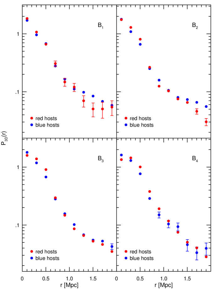
Figure 1: Probability distributions for the locations of satellites surrounding host galaxies in four different stellar mass bins: $10.3\leq\log_{10}\left[M_{\ast}/M_{\odot}\right]<10.6$ ($B_{1}$), $10.6\leq\log_{10}\left[M_{\ast}/M_{\odot}\right]<10.9$ ($B_{2}$), $10.9\leq\log_{10}\left[M_{\ast}/M_{\odot}\right]<11.2$ ($B_{3}$), and $11.2\leq\log_{10}\left[M_{\ast}/M_{\odot}\right]\leq 11.5$ ($B_{4}$). Error bars are standard Poisson errors and are omitted when they are comparable to or smaller than the data points. Approximately 90% of the satellites are found within a 3D distance of $r\leq 2$ Mpc from their hosts and $\lesssim 1$% are found as far as 10 Mpc from their hosts. Note that the slope of $P_{3D}(r)$ changes at $r\sim R_{\rm max}=500$ kpc due to the cylindrical nature of the selection criteria for satellite distances greater than 500 kpc.

Although our satellites are not a random subset of the satellites that would be obtained if 3D selection criteria were used, we can nevertheless anticipate the functional form of the satellite number density profile, $\nu(r)$, from previous work. First, we know that our selection criteria yield a sample of objects that includes both genuine satellites and interlopers. Sales et al. (2007) found that the number density of 3D-selected MRS satellites (i.e., “non-interloper” satellites) was well-fitted by a Navarro, Frenk and White profile (NFW; Navarro, Frenk & White 1995, 1996, 1997) for host-satellite distances $r\lesssim 2~{}r_{200}$. Similarly, Kang et al. (2005) found that when satellites of Milky Way-type halos were selected in 3D, the satellites traced the dark matter distribution well, particularly for radii between $0.1r_{\rm vir}$ and $r_{\rm vir}$. Therefore for small values of $r$, we expect $\nu(r)\propto(r/r_{s})^{-1}(1+r/r_{s})^{-2}$, where $r_{s}$ is the NFW scale radius. For sufficiently large values of $r$, the “satellites” in our sample are, in fact, interlopers. On large scales, then, the form of the probability density for the separation between hosts and satellites should be the same as the probability density for the separation between galaxies as a whole, which is approximated well by a power law (e.g., Hayashi & White 2008). Therefore, for large values of $r$ we expect $\nu(r)\propto r^{-\gamma}$.

To capture the 3D distribution of our entire collection of satellites, we adopt a functional form for the number density that consists of a superposition of an untruncated NFW profile and a power law:

$$\nu(r)\equiv\frac{A}{r/r_{s}\left(1+r/r_{s}\right)^{2}}+\frac{C}{r^{\gamma}}\,,$$ (1)

where $A$ and $C$ are constants. On large scales, the NFW profile falls off as $r^{-3}$ and so long as $\gamma<3$, the number density of satellites at large distances becomes dominated by the interlopers that reside within the tails of the distribution. Throughout, we will refer to these most distant objects as “tail interlopers”. We also note that the NFW profile is technically only valid within the virial radius, but for convenience we extend the NFW profile beyond the virial radii of our hosts in order to smoothly capture the behavior of $\nu(r)$ at radii that are in between those at which the pure NFW profile and the pure power law separately dominate. Below we treat the NFW component of the satellite number counts separately from that of the tail interlopers. To do this, we make the definitions $\nu(r)_{\rm NFW}\equiv A(r/r_{s})^{-1}(1+r/r_{s})^{-2}$ and $\nu(r)_{\rm tail}\equiv Cr^{-\gamma}$. Mathematical expressions for the differential and interior number counts of the satellites in the NFW component and the tail interlopers are given in the Appendix.

3.1 Model Parameters for the Satellite Spatial Distribution

We use a Maximum Likelihood (ML) method to obtain best-fitting model parameters and the corresponding errors for the satellite number density. We evaluate the goodness-of-fit using a combination of the Kolmogorov-Smirnov (KS) statistic and nonparametric bootstrap resampling (e.g., Wall & Jenkins 2003; Babu & Feigelson 2006). Throughout, we obtain the bootstrap samples by repeatedly drawing, with replacements, from the host sample since the satellites are not all independent of each other (i.e., some hosts have more than one satellite). By resampling using the hosts, we insure that an individual bootstrap sample will contain all host-satellite pairs for a given host.

In order to implement the ML fitting procedure, we define a probability density function for the satellite distribution of the form

$$P_{\rm 3D}(r)\equiv(1-f_{\rm tail})P_{\rm NFW}(r)+f_{\rm tail}P_{\rm tail}(r)~{},$$ (2)

where $0\leq f_{\rm tail}\leq 1$ is the fraction of tail interlopers. Here $P_{\rm NFW}(r)$ and $P_{\rm tail}(r)$ are probability density functions for the NFW component and the tail interlopers, respectively. The probability density function has three free parameters: $r_{s}$, $\gamma$, and $f_{\rm tail}$. It also has three geometrical parameters, two of which are known from the selection criteria: $R_{\rm min}$ and $R_{\rm max}$. The third geometrical parameter, $r_{\rm max}$, is the length of the tail of the satellite distribution in 3D, which is unknown in an observational sample. Figure 2 shows the model parameters $r_{s}$ and $\gamma$ from the ML fits that were computed by adopting five different values of $r_{\rm max}$ (1, 2, 3.5, 5, and 7 Mpc), which enclose 83%, 90%, 94%, 96%, and 98% of all satellites, respectively. Errors on the best fit values of $r_{s}$ and $\gamma$ are the corresponding standard errors from the maximum likelihood estimates of the parameters, and are the associated 68% confidence intervals.

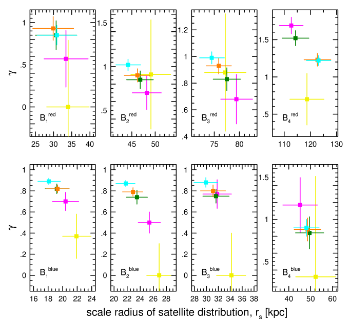
Figure 2: Best-fitting model parameters, $r_{s}$ and $\gamma$, obtained using different values of $r_{\rm max}$: 1 Mpc (yellow), 2 Mpc (pink), 3.5 Mpc (green), 5 Mpc (orange), and 7 Mpc (blue). The best-fitting values of $r_{s}$ are not particularly sensitive to the value of $r_{\rm max}$ that is adopted, and good model fits require the presence of a tail of interlopers in the satellite distribution. The best-fitting values of $\gamma$ are weakly-dependent on the value of $r_{\rm max}$ so long as $r_{\rm max}\geq 3.5$ Mpc (see text).

It is clear from Figure 2 that $r_{s}$ increases with increasing host stellar mass, the best-fitting value of $r_{s}$ is not particularly sensitive to the value of $r_{\rm max}$ that is adopted and, within a given stellar mass bin, the best-fitting value of $r_{s}$ is larger for the satellites of red hosts than it is for the satellites of blue hosts. Also, with the exception of the satellites of the $B_{4}^{\rm red}$ hosts, the best-fitting value of $\gamma$ is only weakly-dependent on the value of $r_{\rm max}$ so long as $r_{\rm max}\geq 3.5$ Mpc. In particular, for $r_{\rm max}=3.5$ Mpc, $\gamma\simeq 0.8$ for all of the satellites except those of the $B_{4}^{\rm red}$ hosts. The $B_{4}^{\rm red}$ hosts have the most massive halos (mean virial mass of $\sim 2.3\times 10^{13}M_{\odot}$) and, hence, the highest velocity dispersions ($\sigma_{v}\sim 320$ km sec^-1). Since the selection criteria reject satellites with relative velocities $|dv|>500$ km sec^-1, it is likely that the sample of satellites around the $B_{4}^{\rm red}$ hosts is incomplete. Therefore, in the case of the $B_{4}^{\rm red}$ hosts, it is likely that our satellite sample is not fully-representative of the satellite distribution around these particular hosts. We also note that, since $r_{s}$ and $\gamma$ both originate with model fits to structure formation in a $\Lambda$CDM universe (for which the mass density field is continuous), $r_{s}$ and $\gamma$ are not fully independent of one another. Of the two, $r_{s}$ is the parameter that we expect to be indicative of the host halo structure, with a strong dependence on the physical properties of the host galaxies. The parameter $\gamma$ primarily reflects the intrinsic clustering of the galaxies. We expect $\gamma$ to have at most a weak dependence on the stellar masses of the host galaxies, and a correspondingly weak correlation with $r_{s}$. This is due to the fact that the power law index describing intrinsic galaxy clustering is only weakly dependent on the physical properties of galaxies (see, e.g., Tables 1 and 2 of Zehavi et al. 2011).

We quantify the quality of the model fits in Figure 2 by computing the KS statistic, combined with 2,500 bootstrap resamplings, which provide unbiased estimates of the goodness-of-fit probabilities for the KS statistics. From this, the best-fitting models in Figure 2 have KS rejection confidence levels $<76$%; i.e., in all cases the fits are good and the goodness-of-fit is unaffected by our choice of the value for $r_{\rm max}$. We also note that acceptable fits to the satellite distribution require the presence of both the NFW and the tail interloper components. That is, acceptable fits to the satellite distribution cannot be obtained if we set $f_{\rm tail}=0$ (an “NFW-only” model) or $f_{\rm tail}=1$ (a “power-law only” model). In particular, if we attempt to fit the satellite distribution solely by an NFW component, the resulting model parameter $r_{s}$ increases monotonically with $r_{\rm max}$ in all of our host stellar mass bins, rather than converging to the values shown in Figure 2. Furthermore, the KS statistics show that the satellite distributions for all of our host stellar mass bins are inconsistent with NFW-only models when we include satellites that lie beyond $r_{\rm max}\gtrsim 2$ Mpc. Finally, we note that for the best-fitting NFW $+$ power law models, the tail interloper fraction ranges from 13% to 24% for the satellites of the red host galaxies, and from 19% to 30% for the satellites of the blue host galaxies.

Figure 3 shows the dependence of the best-fitting values of $r_{s}$ on host stellar mass, which is well-fitted by power laws for the satellites of both red and blue hosts. Formally, $\log_{10}r_{s}^{\rm red}=(0.71\pm 0.05)\log_{10}\left[M_{\ast}/M_{\odot}\right]-(6.0\pm 0.6)$ for the satellites of the red hosts and $\log_{10}r_{s}^{\rm blue}=(0.48\pm 0.07)\log_{10}\left[M_{\ast}/M_{\odot}\right]-(3.8\pm 0.8)$ for the satellites of the blue hosts. From Figure 3, it is also clear that for host stellar masses $M_{\ast}\gtrsim 4\times 10^{10}M_{\odot}$, the satellite distribution around blue hosts is more concentrated than is the satellite distribution around red hosts, where the concentration is given by $c=r_{200}/r_{s}$. It is, of course, important to note that these results are specific to the galaxy formation model that was adopted (i.e., De Lucia & Blaizot 2007) and, hence, they may not constitute a general result for galaxy formation in the context of $\Lambda$CDM.

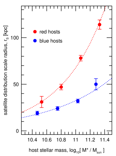
Figure 3: Best-fitting values of the scale radius, $r_{s}$, for the satellite distributions as a function of host color and stellar mass. Here fits to the satellite distributions have been performed using $r_{\rm max}=3.5$ Mpc, but we note from Figure 3 that the value of $r_{s}$ is insensitive to the choice of $r_{\rm max}$. Error bars correspond to 68% confidence intervals from the maximum likelihood parameter estimates. Dotted lines show the best-fitting power laws for the dependence of $r_{s}$ on host stellar mass.

3.2 Satellite Distribution vs. Dark Matter Distribution

In addition to simply determining the spatial distribution of the satellites, we might also hope to use the satellite distribution to place constraints on the concentration of the dark matter halos surrounding the host galaxies. A direct constraint on halo concentration would be possible if the satellites faithfully trace the distribution of the dark matter. A number of studies of the locations of satellite galaxies in SAMs have led to the conclusion that, when selected in 3D, the satellites trace the distribution of CDM halos quite well, both within galaxy clusters (e.g., Gao et al. 2004) and in lower density environments (e.g., Kang et al. 2005; Sales et al. 2007). Hence, the spatial distribution of 3D-selected satellites would seem to be a good tracer of dark matter.

We know, however, that our satellites are not a random subset of all luminous satellites. Since our satellites include only the brightest objects, it is possible that the spatial distribution of these particular objects may lead to different conclusions about the degree to which the satellite distribution traces the distribution of the underlying dark matter. For example, Sales et al. (2007) investigated the average satellite luminosity as a function of radius in their 3D-selected sample. Averaged over their entire sample, Sales et al. (2007) found clear evidence of luminosity segregation, with the average satellite luminosity dropping by a factor of order 2 between the host centers and their halo virial radii. Therefore, faintest and brightest satellites in Sales et al. (2007) have different radial distributions on average.

Here we compute the scale radii for the dark matter halos of our host galaxies and we compare them to the scale radii of the satellite distributions that we obtained above. To compute the scale radii of the halos, we use the dark matter particles to obtain best-fitting NFW mass profiles. Within a given host stellar mass bin, the dark matter particles of the individual hosts were combined into a composite density profile after appropriately scaling each host by $r_{200}$ and $M_{200}$ (see Chapter 7 of Ágústsson (2012). The concentration parameters, $c_{dm}$, of the composite hosts were obtained by fitting NFW profiles, and the scale radii were then defined to be the ratios of the mean halo virial radii to the concentration parameters: $r_{s,dm}=\left<r_{200,dm}\right>/c_{dm}$.

Table 3: NFW Model Parameters for Satellites and Host Dark Matter Halos

Bin	$r_{s,dm}$	$r_{s,sat}$	$c_{dm}$	$c_{sat}$
B${}_{1}^{red}$	$37.4\pm 0.3$	$31\pm 6$	$5.83\pm 0.05$	$7.0\pm 1.4$
B${}_{2}^{red}$	$47.4\pm 0.2$	$47\pm 3$	$5.74\pm 0.02$	$5.8\pm 0.4$
B${}_{3}^{red}$	$63.7\pm 0.2$	$78\pm 3$	$5.42\pm 0.02$	$4.4\pm 0.2$
B${}_{4}^{red}$	$106.1\pm 0.5$	$114\pm 5$	$4.71\pm 0.02$	$4.4\pm 0.2$
B${}_{1}^{blue}$	$36.9\pm 0.1$	$19\pm 2$	$5.15\pm 0.01$	$10.0\pm 1.1$
B${}_{2}^{blue}$	$47.1\pm 0.1$	$24\pm 2$	$4.91\pm 0.01$	$9.6\pm 0.8$
B${}_{3}^{blue}$	$60.4\pm 0.1$	$32\pm 2$	$4.68\pm 0.01$	$8.8\pm 0.6$
B${}_{4}^{blue}$	$79.9\pm 0.2$	$50\pm 6$	$4.59\pm 0.01$	$7.3\pm 0.9$

Figure 4 shows a comparison of the mean values of $r_{s}$ obtained for the host halos using the dark matter particles and the mean values of $r_{s}$ obtained from the satellites (i.e., Figure 3). Since the scale radii of the satellite distributions increase monotonically with stellar mass, it is clear from Figure 4 that the scale radii of the halos also increase monotonically with stellar mass, as expected. From Figure 4, the distribution of satellites around the red hosts traces the dark matter distribution well. However, the scale radii for the dark matter distributions surrounding the blue hosts exceed those of the satellites by a factor of $\sim 2$ in all four stellar mass bins. This leads to the conclusion that, when selected in redshift space, the satellites of the blue MRS host galaxies have a spatial distribution that is approximately twice as concentrated as the dark matter surrounding the hosts. Table 3 summarizes the mean values of the scale radii of the halo dark matter distributions, the mean values of the scale radii of the satellite distributions, and the corresponding mean values of the concentration parameters.

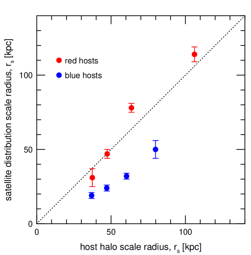
Figure 4: Comparison of scale radii for the satellite distributions and the dark matter halos that surround the hosts. The satellites of red hosts are distributed similarly to the dark matter; the satellites of blue hosts have distributions that are more concentrated than the dark matter by a factor of $\sim 2$.

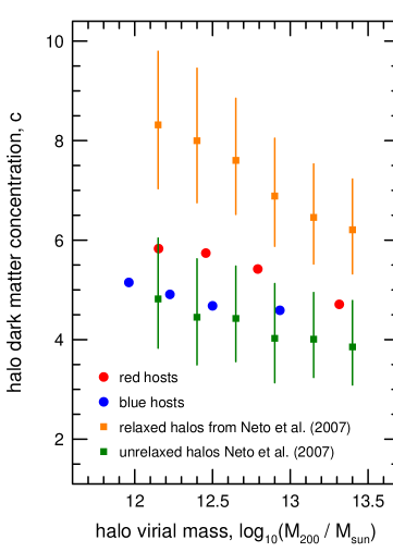
Figure 5: Comparison of concentration parameters for the halos of our host galaxies with those obtained for MRS halos by Neto et al. (2007). Error bars for the mean host halo concentration parameters are omitted because they are smaller than the sizes of the data points. Vertical lines indicate the ranges of values for $c$ that correspond to the 25th and 75th percentiles from Neto et al. (2007).

It should be kept in mind that, just as our satellites are not a random sample of all satellite galaxies, our host galaxies are also not a random sample of “average” galaxies. Instead, our hosts are large, bright galaxies that are relatively isolated within their local regions of space. Because of this we would not necessarily expect the properties of the host dark matter halos to be identical to the average population in the MRS. To explore this, we compare the mean concentration parameters that we obtain for our host halos to the mean concentration parameters obtained by Neto et al. (2007) for all MRS halos. Shown in Figure 5 are the mean values of the concentration parameters of our host halos as a function of $M_{\rm 200}$. Also shown in Figure 5 are the mean values of the concentration parameters and the corresponding 25th to 75th percentile ranges for both relaxed and unrelaxed MRS halos from Neto et al. (2007). Within the mass range of the halos of our host galaxies, Neto et al. (2007) find that a fraction $f_{\rm unrelax}\simeq 0.25$ of all MRS halos are unrelaxed.

From Figure 5, the dependence of the mean concentration parameter on $M_{\rm 200}$ for the halos of our blue hosts is consistent with the results for unrelaxed MRS halos. Therefore, it is likely that our sample of blue host galaxies is dominated by objects with unrelaxed halos, in which case we would not necessarily expect the spatial distribution of the satellites to trace the dark matter distribution. For our red hosts, the dependence of the mean halo concentration parameter on $M_{\rm 200}$ is consistent with the upper (75%) bound on the value of $c$ for unrelaxed MRS halos, but is slightly below the lower (25%) bound on the value of $c$ for all MRS halos. This suggests that the halos of our red hosts consist of a mixture of relaxed and unrelaxed halos, with a larger fraction of the halos of red hosts being unrelaxed in comparison to the complete sample of MRS halos (i.e., $f_{\rm unrelax}>0.25$ for the halos of our red host galaxies).

To the degree that our results and those of Sales et al. (2007) can be directly compared, we find broad general agreement. Sales et al. (2007) concluded that, when averaged over their entire 3D-selected sample, the distribution of MRS satellites was sightly less concentrated than the average host dark matter halo ($c_{sat}\sim 5.6$ vs. $c_{dm}\sim 8.1$). They also found that dividing their host sample in half by either halo mass or host galaxy luminosity resulted in little change to the inferred concentration for the satellite distribution. Sales et al. (2007) did not investigate the concentration of the satellite distribution as a function of host stellar mass or color, so a direct comparison of our results and theirs is limited. From Table 3, the concentration of our satellite distributions decreases somewhat with host halo mass, however the effect is marginal (less than $2\sigma$). Therefore, like Sales et al. (2007), we find no strong evidence that the concentration of the satellite distribution varies as a function of host halo mass. When we compute the mean value of the concentration parameter for our entire satellite distribution, weighted according to the number of satellites within $r_{200}$ in each stellar mass bin, the result is similar to the mean value of the concentration for our entire host dark matter halo sample, weighted by the number of hosts within each stellar mass bin: $c_{sat}=6.3$ vs. $c_{dm}=5.2$. That is, when averaged over the entire sample, the distribution of our satellites is slightly more concentrated than is the dark matter that surrounds the host galaxies; however, the halos of our host galaxies are somewhat less concentrated than are the halos studied by Sales et al. (2007).

4 Summary

We investigated the spatial locations of the satellites of relatively isolated host galaxies selected from the first Millennium Run simulation (MRS). The satellites were identified using redshift space selection criteria, in direct analogy with spectroscopically selected satellite galaxies in large redshift surveys. Our primary conclusions center on the answers to two questions: [1] How does the spatial distribution of the satellites depend on the color and stellar mass of the host galaxy? [2] To what degree does the satellite distribution trace the distribution of the dark matter surrounding the halos of the host galaxies? We summarize the answers to these questions below.

As expected from previous work, the locations of the satellites are well-fitted by a combination of an NFW profile and a power law. The NFW profile characterizes the genuine satellites, while the power law characterizes the interlopers (or “false” satellites). The best-fitting values of the NFW scale radius, $r_{s}$, are insensitive to the maximum distance, $r_{\rm max}$, that we adopt in our analysis. With the exception of the satellites of the most massive red hosts, the best-fitting power law index, $\gamma$, is also largely insensitive to the value of $r_{\rm max}$ that is adopted, provided $r_{\rm max}\geq 3.5$ Mpc. That is, we need a sufficient number of interlopers to be present in the tail of the distribution in order for the fit to converge to a single value of $\gamma$. The best-fitting values of the NFW scale radius are functions of both the stellar masses and the rest-frame colors of the host galaxies. At fixed host stellar mass, the values of $r_{s}$ for the satellites of red hosts exceed those for the satellites of blue hosts. The dependence of $r_{s}$ on host stellar mass is well-fitted by a power law, but the index of the power law differs for the satellites of the red and blue hosts: $r_{s}^{\rm red}\propto\left(M_{\ast}/M_{\odot}\right)^{0.71\pm 0.05}$ and $r_{s}^{\rm blue}\propto\left(M_{\ast}/M_{\odot}\right)^{0.48\pm 0.07}$. These relationships constitute predictions for the dependence of the spatial distribution of satellite galaxies that should be observed in our universe, if the satellite galaxies have been selected from redshift space, if the mass of our universe is dominated by CDM, and if the adopted SAM (i.e., De Lucia & Blaizot 2007) is representative of galaxy formation in our universe. In particular, we expect the spatial distribution of the satellites of blue host galaxies with $M_{\ast}\gtrsim 4\times 10^{10}M_{\odot}$ would be significantly more concentrated than the spatial distribution of the satellites of red host galaxies with similar stellar masses.

When we compare the scale radii of the satellite distributions to the scale radii of the dark matter halos that surround the host galaxies, we find that the satellites of red host galaxies trace the dark matter distribution well. However, in the case of the satellites of blue host galaxies, the spatial distribution of the satellites is more concentrated than is the halo dark matter by a factor of $\sim 2$. This suggests that, when selected using redshift space criteria, the spatial distribution of satellite galaxies may be a biased tracer of the dark matter distribution that surrounds blue host galaxies. From the dependence of the host halo concentration on virial mass, it is likely that our sample of blue hosts is dominated by objects with unrelaxed halos. Therefore, we would not necessarily expect the spatial distribution of the satellites of blue host galaxies to trace the distribution of the halo dark matter. We caution, however, that this result is based upon the use of a particular galaxy formation model and therefore may not be a general result for $\Lambda$CDM.

By their nature, SAMs attempt to model the galaxy formation process in a manner that is computationally efficient, but which necessarily relies on simplifying assumptions and a large number of parameters. Because of the large number of parameters associated with SAMs (i.e., 10 to 30), it is challenging to fully explore all of the associated parameter space. While highly detailed in their treatment of the relevant physics, hydrodynamical simulations of galaxy formation are much more computationally expensive than SAMs. Although a great deal of progress has been made in recent years, hydrodynamical simulations must still rely on “subgrid physics”; i.e., parameterization on scales smaller than the resolution scale due to the fact that it is not currently possible to simulate the full range of physical scales needed to describe galaxy formation within a large, cosmologically-appropriate volume. Because neither method is perfect, neither method provides definitive answers to all of the questions surrounding the history of galaxy formation. As such, SAMs and hydrodynamical simulations are highly complementary tools at present. See, e.g., Wechsler & Tinker (2018) for a comprehensive review.

Because of the complementarity of SAMs and hydrodynamical simulations, and since no one SAM or hydrodynamical simulation currently provides the definitive description of galaxy formation in our universe, it will be interesting in the future to compare the results from this work to similar analyzes of simulations that incorporate different SAMs, as well as to the results from high-resolution hydrodynamical simulations. Other SAMs to which our results could be compared include the Guo et al. (2011) SAM for the Bruzual & Charlot (2003) and Maraston (2005) population synthesis models. In particular, Henriques et al. (2012) used the Guo et al. (2011) SAM in their light cones of the MRS. The Guo et al. (2011) SAM was also used by Guo et al. (2013) when scaling of the growth of structure in the MRS to parameters that are consistent with the seven-year Wilkinson Microwave Anisotropy Probe (WMAP) data. It was also used by Henriques et al. (2015) when updating the Munich galaxy formation model to the Planck first-year cosmology. High-resolution hydrodynamical simulations to which this work could be compared include the Illustris project (e.g., Genel et al. 2014; Vogelsberger et al. 2014), the Illustris TNG project (e.g., Weinberger et al. 2017, Pillepich et al. 2018), the GIMIC project (Crain et al. 2009), the OWL project (Schaye et al. 2010), and the EAGLE project (Schaye et al. 2015; Crain et al. 2015). GIMIC makes use of the dark matter structure formation from select regions of the MRS, while Illustris, IllustrisTNG, OWLS, and EAGLE are independent of the MRS.

Appendix A Appendix

Here we present mathematical expressions for the differential and interior number counts of the satellites in the NFW component of the satellite distribution, as well as the tail interlopers. Taking $\nu(r)$ to be the satellite number density profile, the differential number count is simply the number of satellites found within the infinitesimal interval $\left[r,r+dr\right]$,

$$dN(r)=\int_{S}\nu(r)~{}dS~{}dr~{}dN(r)=4\pi\left[r^{2}-r\sqrt{{\cal R}\left(r^{2}-R_{\rm max}^{2}\right)}\,\right]~{}\nu(r)~{}dr,$$ (A1)

where $S$ is the area of the spherical surface at radius $r$ contained within a cylinder of radius $R_{\rm max}$ and ${\cal R}(x)$ is the ramp function: ${\cal R}(x)=x$ for $x\geq 0$ and ${\cal R}(x)=0$ otherwise (see Ágústsson 2012). The interior number count is simply the cumulative number of satellites that are enclosed within a 3D distance $r$,

$$N(<r)=\int_{0}^{r}dN(r)~{}.$$ (A2)

Using Equations (A1) and (A2), the 3D differential and interior number counts of the satellites in the NFW component are given by

$$dN_{\rm NFW}(r)=4\pi Ar_{s}~{}\frac{r-\sqrt{{\cal R}(r^{2}-R_{\rm max}^{2})}}{\left(1+r/r_{s}\right)^{2}}~{}dr$$ (A3)

$$N_{\rm NFW}(<r)=4\pi Ar_{s}^{3}\left[\ln\left(1+r/r_{s}\right)-\frac{r/r_{s}}{1+r/r_{s}}-g_{\rm NFW}(r)\right]~{},$$ (A4)

where

$$g_{\rm NFW}(r)=\left\{\begin{array}[]{ll}0&\mbox{$r\leq R_{\rm max}$}\\ {\rm cosh}^{-1}\left(\frac{r}{R_{\rm max}}\right)-\frac{\sqrt{r^{2}-R_{\rm max}^{2}}}{r+r_{s}}-\frac{r_{s}~{}\cos^{-1}\left(\frac{rr_{s}+R_{\rm max}^{2}}{(r+r_{s})R_{\rm max}}\right)}{\sqrt{R_{\rm max}^{2}-r_{s}^{2}}}&\mbox{$r>R_{\rm max}$~{}.}\end{array}\right.$$ (A5)

The 3D differential and interior number counts of the tail interlopers are given by

$$dN_{\rm tail}=4\pi Cr^{-\gamma}\left[r^{2}-r\sqrt{{\cal R}(r^{2}-R_{\rm max}^{2})}\,\right]~{}dr$$ (A6)

$$N_{\rm tail}(<r)=4\pi C\left[(3-\gamma)^{-1}r^{(3-\gamma)}-R_{\rm max}^{(3-\gamma)}\,g_{\rm tail}(r/R_{\rm max})\right]~{},$$ (A7)

where

$$g_{\rm tail}(x)=\left\{\begin{array}[]{lll}0&\mbox{$x\leq 1$}\\ \frac{1}{2}\left[x\sqrt{x^{2}-1}-{\rm cosh}^{-1}(x)\right]&\mbox{$x>1$, $\gamma=1$}\\ \frac{1}{(3-\gamma)(\gamma-1)}\left[\frac{\sqrt{x^{2}-1}}{x^{\gamma}}\left\{(\gamma-1)x^{2}+1)\right\}+\frac{\gamma}{2}B\left(x^{-2};\frac{\gamma+1}{2},\frac{1}{2}\right)-\frac{\sqrt{\pi}\Gamma\left(\frac{\gamma+1}{2}\right)}{\Gamma\left(\frac{\gamma}{2}\right)}\right]&\mbox{$x>1$, $\gamma\neq 1$~{}.}\end{array}\right.$$ (A8)

Here $B(y;a,b)\equiv\int_{0}^{y}t^{a-1}\left(1-t\right)^{b-1}~{}dt$ is the incomplete Beta function. These expressions can also be found in Chapter 7 of Ágústsson (2012).

References

- Agustsson (2012) Ágústsson, I. 2012, PhD dissertation, Boston University
- Agustsson & Brainerd (2006a) Ágústsson, I. & Brainerd, T. G., 2006, ApJ, 644, L25
- Agustsson & Brainerd (2006b) Ágústsson, I. & Brainerd T. G., 2006, ApJ, 650, 550
- Agustsson & Brainerd (2010) Ágústsson, I. & Brainerd T. G., 2010, ApJ, 709, 1321 (AB10)
- Agustsson & Brainerd (2010) Ágústsson, I. & Brainerd, T. G., 2011, ISRN Astronomy & Astrophysics, vol. 2011, id # 958973 (doi: 10.5402/2011/958973)
- Azzaro et al. (2007) Azzaro, M., Patiri, S. G., Prada, F., & Zentner, A. R. 2007, MNRAS, 376, L43
- Babu & Feigelson (2006) Babu, G. J. & Feigelson, E. D. 2006, in ASP Conf. Series Vol. 351, Astronomical Data Analysis Software and Systems XV, eds. C. Gabriel, C. Arviset, D. Ponz & S. Enrique, 127
- Bett et al. (2007) Bett, P., Eke, V., Frenk, C. S., Jenkins, A., Helly, J. & Navarro, J. 2007 MNRAS, 376, 215
- Blaizot et al. (2005) Blaizot, J., Wadadekar, Y., Guiderdoni, B., Colombi, S. T., Bertin, E., Bouchet, F. R., Devriendt, J. E. G., & Hatton, S. 2005, MNRAS, 360, 159
- Brainerd & Specian (2003) Brainerd, T. G. & Specian, M. A. 2003, ApJ, 593, L7
- Brainerd (2005) Brainerd, T. G. 2005, 628, L101
- Bruzual & Charlot (2003) Bruzual, G. & Charlot, S. 2003, MNRAS, 344, 1000
- Chabrier (2003) Chabrier, G. 2003, PASP, 115, 763
- Conroy et al. (2005) Conroy, C. et al. 2005, ApJ, 635,982
- Conroy et al. (2007) Conroy, C. et al. 2007, ApJ, 654, 153
- Conroy et al. (2009) Conroy, C., Gunn, J. E. & White, M. 2009, ApJ, 699, 486
- Crain et al. (2009) Crain, R. A. et al. 2009, MNRAS, 399, 1773
- Crain et al. (2015) Crain, R. A. et al. 2015, MNRAS, 450, 1937
- Croton et al. (2006) Croton, D. J., et al. 2006, MNRAS, 365, 11
- De Lucia & Blaizot (2007) De Lucia, G. & Blaizot, J. 2007, MNRAS, 375, 2
- Fukugita et al. (1996) Fukugita, M., Ichikawa, T., Gunn, J. E., Doi, M., Shimasaku, K. & Schneider, D. P. 1996, AJ, 111, 1748
- Gao et al. (2004) Gao, L., DeLucia, G., White, S. D. M. & Jenkins, A. 2004, MNRAS, 352, L1
- Guo et al. (2011) Guo, Q. et al. 2011, MNRAS, 413, 101
- Guo et al. (2013) Guo, Q. et al. 2013, MNRAS, 428, 1351
- Genel et al. (2014) Genel, S. et al. 2014, MNRAS, 445, 175
- Hayashi & White (2008) Hayashi, E. & White, S. D. M. 2008, MNRAS, 388, 2
- Henriques et al. (2012) Henriques, B. M. B. et al. 2012, MNRAS, 421, 2904
- Henriques et al. (2015) Henriques, B. M. B. et al. 2015, MNRAS, 451, 2663
- Hogg et al. (2001) Hogg, D. W., Finkbeiner, D. P., Schlegel, D. J. & Gunn, J. E. 2001, AJ, 122, 2129
- Kang et al. (2005) Kang, X., Mao, S., Gao, L. & Jing, Y. P. 2005, AA, 437, 383
- Klypin & Prada (2009) Klypin, A. & Prada, F. 2009, ApJ, 690, 1488
- Maraston (2005) Maraston, C. 2005, MNRAS, 362, 799
- McKay et al. (2002) McKay, T. A. et al. 2002, ApJ, 571, L85
- More et al. (2009) More, S., van den Bosch, F. C., Cacciato, M., Mo, H. J., Yang, X. & Li, R. 2009, MNRAS, 392, 801
- More et al. (2011) More, S., van den Bosch, F. C., Cacciato, M., Skibba, R., Mo, H. J. & Yang, X. 2011, MNRAS, 410, 210
- Nagai & Kravtsov (2005) Nagai, D. & Kravtsov, A. V. 2005, ApJ, 618, 557
- Navarro et al. (1995) Navarro, J. F., Frenk, C. S., White, S. D. M., 1995, MNRAS, 275, 720
- Navarro et al. (1996) Navarro, J. F., Frenk, C. S., White, S. D. M., 1996, ApJ, 462, 563
- Navarro et al. (1997) Navarro, J. F., Frenk, C. S., White, S. D. M., 1997, ApJ, 490, 493
- Neto et al. (2007) Neto, A. F., Gao, L., Bett, P., Cole, S., Navarro, J. F., Frenk, C. S., White, S. D. M., Springel, V. & Jenkins, A. 2007, MNRAS, 381, 1450
- Norberg et al. (2008) Norberg, P., Frenk, C. S. & Cole, S. 2008, MNRAS, 383, 646
- Prada et al. (2003) Prada, F., Vitvitska, M., Klypin, A., Holtzman, J. A., Schlegel, D. J., Grebel, E. K., Rix, H.-W., Brinkmann, J., McKay, T. A. & Csabai, I. 2003, ApJ, 598, 260
- Pillepich et al. (2018) Pillepich, A. et al. 2018, MNRAS, 473, 4077
- Sales & Lambas (2004) Sales, L. & Lambas, D. G. 2004, MNRAS, 348, 1236
- Sales & Lambas (2009) Sales, L. & Lambas, D. G. 2009, MNRAS, 395, 1184
- Sales et al. (2007) Sales, L., Navarro, J. F., Lambas, D. G., White, S. D. M. & Croton, D. J. 2007, MNRAS, 382, 1901
- Schaye et al. (2010) Schaye, J., et al. 2010, MNRAS, 402, 1536
- Schaye et al. (2015) Schaye, J. et al. 2015, MNRAS, 446, 521
- Siverd et al. (2009) Siverd, R., Ryden, B. & Gaudi, B. S. 2009, preprint, submitted to ApJ (arXiv:0903.2264)
- Smith et al. (2002) Smith, J. A. et al. 2002, AJ, 123, 2121
- Springel et al. (2005) Springel, V., et al. 2005, Nature, 435, 629
- Strateva et al. (2001) Strateva I., et al., 2001, ApJ, 122, 1861
- Strauss et al. (2002) Strauss, M. A., Weinberg, D. H. et al. 2002, AJ, 124, 1810
- van den Bosch et al. (2004) van den Bosch, F. C., Norberg, P., Mo, H. J. & Yang, X. 2004, MNRAS, 352, 1302
- Velliscig et al. (2015) Velliscig, M., Cacciato, M., Schaye, J., et al., 2015, MNRAS, 454, 3328
- Vogelsberger et al. (2014) Vogelsberger, M. et al. 2014, MNRAS, 444, 1518
- Wall & Jenkins (2003) Wall, J. V. & Jenkins, C. R. 2003, Practical Statistics for Astronomers (Cambridge University Press)
- Wechsler & Tinker (2018) Wechsler, R. H. & Tinker, J. L. 2018, ARAA, vol. 56, submitted (arXiv:1804.03097)
- Weinberger et al. (2017) Weinberger, R. et al. 2017, MNRAS, 465, 3291
- Weinmann et al. (2006) Weinmann, S. M., van den Bosch, F. C., Yang, X., & Mo, H. J., 2006, MNRAS, 366, 2
- York et al. (2000) York, D. G. et al. 2000, AJ, 120, 1579
- Zehavi et al. (2011) Zehavi, I. et al. 2011, ApJ, 736, 59