Spitzer Microlensing Program as a Probe for Globular Cluster Planets.
Analysis of OGLE-2015-BLG-0448

Abstract

The microlensing event OGLE-2015-BLG-0448 was observed by Spitzer and lay within the tidal radius of the globular cluster NGC 6558. The event had moderate magnification and was intensively observed, hence it had the potential to probe the distribution of planets in globular clusters. We measure the proper motion of NGC 6558 (${\mbox{\boldmath$\mu$}}_{cl}(N,E)=(+0.36\pm 0.10,+1.42\pm 0.10)\,{\rm mas}\,{\rm yr}^{-1}$) as well as the source and show that the lens is not a cluster member. Even though this particular event does not probe the distribution of planets in globular clusters, other potential cluster lens events can be verified using our methodology. Additionally, we find that microlens parallax measured using OGLE photometry is consistent with the value found based on the light curve displacement between Earth and Spitzer.

1. Introduction

The Spitzer gravitational microlensing project has as its principal aim the determination of the Galactic distribution of planets (Gould et al., 2014). This primarily means using Spitzer to measure “microlens parallaxes” ${\mbox{\boldmath$\pi$}}_{\rm E}$ and thereby estimate the distances of the individual lenses. By comparing this overall distance distribution to the one restricted to events showing planetary signatures one can determine whether planets are more common in, for example, the Galactic disk or the bulge (Calchi Novati et al., 2015a; Yee et al., 2015). Among the 170 microlensing events observed during the 2015 campaign (Calchi Novati et al., 2015b), one event showed a potential for a very different probe of the “Galactic distribution of planets”, namely of the frequency of planets in globular clusters (relative to disk or bulge stars). The event OGLE-2015-BLG-0448 lay projected against the globular cluster NGC 6558 (Fig. 1), and therefore the lens was potentially a member of this cluster. The lens mass is measured if one knows the relative lens-source parallax and the angular size of the Einstein ring radius (Refsdal, 1964). In the case of a globular cluster lens, one can in principle derive the lens mass based on the Einstein timescale measurement alone (knowing the cluster distance and proper motion from the literature; Paczyński, 1994). In reality, significant uncertainties are introduced by the dispersion of bulge source proper motions that is comparable to the cluster proper motion.

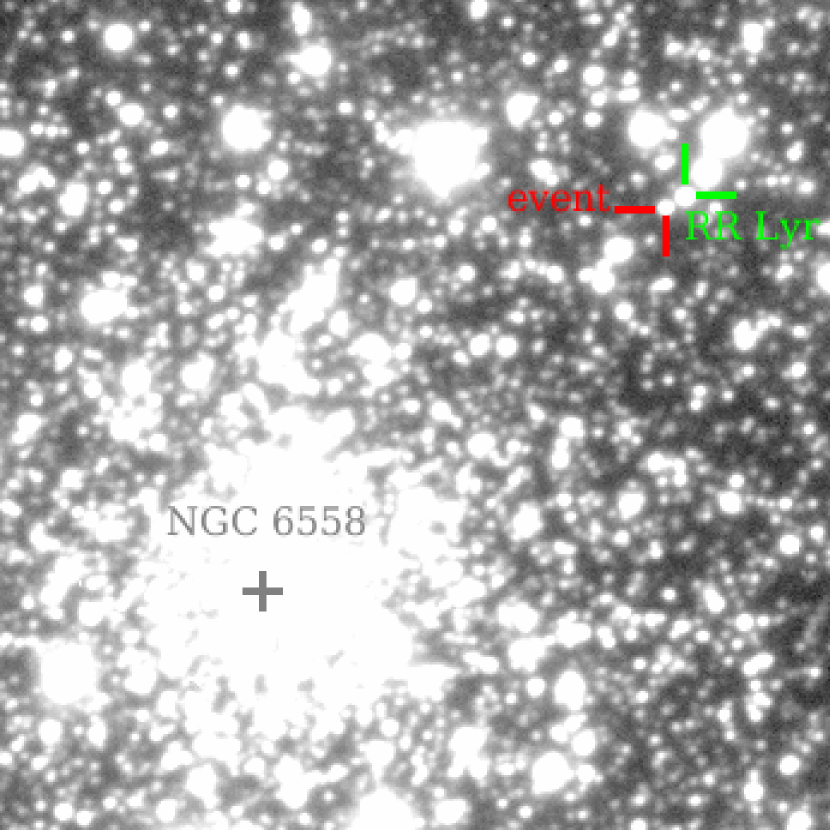
Figure 1.— Finding chart for OGLE-2015-BLG-0448. We marked the center of the globular cluster NGC 6558 (core radius and half-light radius of $0\farcm 03$ and $2\farcm 15$, respectively), the event (baseline brightness $I=16.34~{}{\rm mag}$), and the neighboring RR Lyr star OGLE-BLG-RRLYR-14873 (mean brightness $I=15.52~{}{\rm mag}$). North is up, East is left. The image is $1\farcm 5\times 1\farcm 5$.

Here we present a new method to determine whether the lens from a microlensing event seen projected against a cluster is in fact a cluster member, employing observations of the Spitzer spacecraft as a “microlensing parallax satellite”. The method is to compare the direction of the heliocentric projected velocity $\tilde{\bf v}_{\rm hel}$ with that of the proper motion of the cluster relative to the microlensed source ${\mbox{\boldmath$\mu$}}_{cl,s}$. As is well known, $\tilde{\bf v}_{\rm hel}$ can be subject to a four-fold degeneracy in direction (Refsdal, 1966; Gould, 1994), but within those degenerate solutions can be very precisely measured by a parallax satellite (Calchi Novati et al., 2015a). Therefore, if ${\mbox{\boldmath$\mu$}}_{cl,s}$ can also be measured precisely, the hypothesis of the cluster lens can be tested with high precision.

The analyzed event was unusually sensitive to planets, independent of the possibility that the lens might be a cluster member. First, the source star is a low-luminosity giant, meaning that photometry from both ground and space was unusually precise. Second, it reached magnification $A_{\rm max}\approx 13$ as seen from both Earth and Spitzer. Such moderate magnification events are substantially more sensitive to planets than typical events (Mao & Paczyński, 1991; Gould & Loeb, 1992). The combination of these factors led to relatively intensive monitoring from the ground and exceptionally intensive monitoring from Spitzer, which further increased the event’s planet sensitivity. We show that residuals for Spitzer data and point-lens model can be fitted with a Saturn-mass ratio double-lens model. We do not claim planet detection because Spitzer photometry of neighboring constant stars shows systematic trends that could mimic the planetary signal if superimposed on a purely point lens (Paczyński, 1986) light curve. The only known planet in a globular cluster is in a system of white dwarf and pulsar (Richer et al., 2003; Nascimbeni et al., 2012).

The light curve of OGLE-2015-BLG-0448 is analyzed here for two different purposes: to measure the microlens parallax and to estimate the planet sensitivity. The available ground-based data are survey observations by the Optical Gravitational Lens Experiment (OGLE) project and the follow-up observations taken by three groups: Microlensing Follow Up Network ($\mu$FUN), RoboNet, and Microlensing Network for the Detection of Small Terrestrial Exoplanets (MiNDSTEp). For parallax determination we use only OGLE photometry; Survey long-term monitoring is crucial in deriving event timescale and parallax. OGLE photometry is also well-characterized and systematic trends in the data are at a relatively low level. On the other hand, the planet sensitivity is the highest if many data points are taken close to the light curve maximum (Griest & Safizadeh, 1998). The field including OGLE-2015-BLG-0448 is observed rarely by the OGLE survey, hence, the OGLE light curve does not contribute much to the planet sensitivity. The follow-up data give us much more information with this regard: they are taken from multiple sites allowing better time-coverage and reduced dependence on weather at a single site, and they can be also taken with much higher cadence because many telescopes are targeted on a single event. However, extending the event coverage by most of the follow-up observatories is not possible because of their limited resources or the chosen observing strategy. Additionally, many events get faint far from the peak and the smaller telescopes photometry in dense stellar region may be affected by systematic trends that could corrupt the measurements of the event timescale and parallax. Hence, the ground-based measurements of the event timescale and parallax are best done with the OGLE data only, but follow-up observations are included for the planet sensitivity calculations.

We describe the observations in Section 2. In Section 3 we analyze first the ground-based light curve alone and then the combined Spitzer and ground-based light curves. We measure the microlens parallax ${\mbox{\boldmath$\pi$}}_{\rm E}$ and the closely related relative velocity projected on the observer plane $\tilde{\bf v}_{\rm hel}$, which are required to determine the lens location. In Section 4, we measure the proper motions of NGC 6558 and of the source star in the same frame of reference, which allows us to determine their relative proper motion, ${\mbox{\boldmath$\mu$}}_{cl,s}$. The fact that its direction is inconsistent with that of $\tilde{\bf v}_{\rm hel}$ proves that the lens is not in the cluster. Having eliminated this possibility, in Section 5, we demonstrate that the lens (host star) almost certainly lies in the Galactic bulge, implying that it is a low-mass star and that the tentative planet would therefore be a cold Neptune. The planet sensitivity of the event, which will eventually be required for the determination of the Galactic distribution of planets is analyzed in Section 6. We conclude in Section 7. We discuss the tentative planet detection in Appendix A.

2. Observations

2.1. OGLE Alert and Observations

On 2015 March 20, the OGLE survey alerted the community to a new microlensing event OGLE-2015-BLG-0448 based on observations with the 1.4 deg² camera on the 1.3m Warsaw Telescope at the Las Campanas Observatory in Chile (Udalski et al., 2015) using its Early Warning System (EWS) real-time event detection software (Udalski et al., 1994; Udalski, 2003). Most OGLE observations were taken in the $I$ band, and $V$ band observations are only used to determine the source properties. At equatorial coordinates ($18^{\rm h}10^{\rm m}14\fs 38,~{}-31\arcdeg 45\arcmin 09\farcs 4$), Galactic coordinates $(0\fdg 20,\,-6\fdg 01)$, this event lies in the OGLE field BLG573, implying that it is observed at roughly once per two nights (cf. Fig. 15 from Udalski et al. 2015). We analyze 65 datapoints collected during the 2015 bulge season before ${\rm HJD}^{\prime}\equiv{\rm HJD}-2450000=7301.6$ (Oct $6^{\rm th}$) and supplement them with 73 datapoints from 2014. To account for underestimated uncertainties that are reported by the image-subtraction software we multiplied the uncertainties by a factor of $1.8$, so that the point-lens parallax model results in $\chi^{2}/dof\approx 1$.

2.2. Spitzer Observations

OGLE-2015-BLG-0448 was announced by the Spitzer team as a target on 2015 May 19 UT 20:45 (${\rm HJD}^{\prime}=7162.4$), about 2.5 weeks before the beginning of the 2015 Spitzer observations (proposal ID: 11006, PI: Gould) and 3.5 weeks before this particular object could be observed (${\rm HJD}^{\prime}=7187.1$) due to Sun-angle restrictions. The reason for this early alert was that the source was bright and appeared to be heading for relatively high magnification, making it relatively sensitive to planets. According to the protocols of Yee et al. (2015), planet detections (and sensitivity) can only be claimed for observations after the Spitzer public selection date (or if the event was later selected “objectively”, which was not possible for this event due to low OGLE cadence). Furthermore, without a public alert, the event would not have attracted attention for the intensive follow-up required to raise sensitivity to planets. The Spitzer cadence was set at once per day, and this cadence was followed during the second week of the campaign, when OGLE-2015-BLG-0448 came within Spitzer’s view.

However, the Yee et al. (2015) protocols also prescribe that once all specified observations are scheduled, any additional time should be allocated to events that are achieving relatively high magnification during the next week’s observing window, with the cadence of these events rank-ordered by the $1\,\sigma$ lower limit of expected magnification. Based on this, OGLE-2015-BLG-0448 was slated for cadences of 4, 8, 8, and 4 per day during weeks 3, 4, 5, and 6, respectively. Due to the fact that it lay far to the east, OGLE-2015-BLG-0448 could be observed right to the end of the campaign at ${\rm HJD}^{\prime}=7222.78$. Altogether we collected 210 epochs, each consisting of six 30s dithers. The photometry was obtained with a modified version of Calchi Novati et al. (2015b) pipeline, which fits the centroid and brightness of every stars for each frame separately. The errorbars reported by this pipeline are a nearly linear function of the measured flux, hence, we assumed the errorbars are equal to the value of this linear function multiplied by the factor $4.3$ that brings $\chi^{2}/dof$ to 1 for the parallax point source model.

2.3. $\mu$FUN Observations

As one of the few very bright Spitzer events, and one that was not intensively monitored by microlensing surveys (and so required follow-up to achieve reasonable planet sensitivity), OGLE-2015-BLG-0448 was targeted by $\mu$FUN, including the following five small-aperture telescopes from Australia and New Zealand: the Auckland Observatory 0.5m (R band), the Farm Cove Observatory 0.36m (unfiltered, Pakuranga), the PEST Observatory 0.3m (unfiltered, Perth), the Possum Observatory 0.36m (unfiltered, Patutahi), and the Turitea Observatory 0.36m (R band, Palmerston North). $\mu$FUN also observed the event regularly using the dual ANDICAM optical/IR camera on the 1.3m SMARTS telescope at CTIO, Chile. Almost all the optical observations are in the $I$ band. The IR observations are all in $H$ but these are for source characterization and are not used in the fits. Follow-up photometric data were also taken by the Wise Collaboration on their 1.0m telescope at Mitzpe Ramon, Israel. A limited number of additional measurements were taken using two 0.7m MINiature Exoplanet Radial Velocity Array (MINERVA) telescopes at Mt. Hopkins, USA (Swift et al., 2015).

All $\mu$FUN data were reduced using DoPhot software (Schechter et al., 1993). The photometry of this event is hampered by an ab-type RR Lyrae variable OGLE-BLG-RRLYR-14873 (Kunder et al., 2008; Soszyński et al., 2011) that lies projected at $2\farcs 4$ from the event (Fig. 1), has $I$-band amplitude of $0.23\,{\rm mag}$, and period of $0.67\,{\rm d}$. Because DoPhot fits separately for the flux of each star at each epoch, it is ideally suited to remove the effects of this neighboring variable, even when the point spread functions (PSFs) of the two stars overlap, as they frequently do for the smaller $\mu$FUN telescopes. By contrast, plain vanilla image-subtraction algorithms fit only for variations centered at the source and so include residuals from neighboring PSFs, if these overlap. Unfortunately, DoPhot failed to separately identify the source in PEST data and so these could not be used. Possum data showed unusual scatter and were also excluded.

2.4. RoboNet Observations

RoboNet observed OGLE-2015-BLG-0448 from three Las Cumbres Observatory Global Telescope Network (LCOGT) sites in its southern hemisphere ring of 1.0m telescopes: CTIO/Chile, SAAO/South Africa, and Siding Spring/Australia (Brown et al., 2013). Different telescopes at the same site are indicated as A, B, and C. Two CTIO telescopes (A and C) were equipped with the new generation of Sinistro imagers that consist of $4{\rm k}\times 4{\rm k}$ Fairchild CCD-486 Bl CCDs and offer a field of view of $27^{\prime}\times 27^{\prime}$. Other telescopes support SBIG STX-16803 cameras with Kodak KAF-16803 front illuminated $4{\rm k}\times 4{\rm k}$ pix CCDs, used in bin $2\times 2$ mode with a field of view of $15.8^{\prime}\times 15.8^{\prime}$. All observations were made using SDSS-$i^{\prime}$ filters. Standard debiasing, dark-subtraction, and flat fielding were performed for all datasets by the LCOGT Imaging Pipeline, after which Difference Image Analysis was conducted using the RoboNet Pipeline, which is based around DanDIA (Bramich, 2008; Bramich et al., 2013).

LCOGT employed its TArget Prioritization algorithm (Hundertmark et al., 2015) to select a sub-set of events from the Spitzer target list based on their predicted sensitivity to planets, which were drawn from Spitzer targets that fell in regions of lower survey observing cadence. OGLE-2015-BLG-0448 was given priority because it fell within such a region, and due to the added scientific value of the proximity of the globular cluster.

2.5. MiNDSTEp Observations

The MiNDSTEp consortium observed OGLE-2015-BLG-0448 using the Danish 1.54 m telescope at ESO’s La Silla Observatory, Chile and the 0.35m Schmidt-Cassegrain telescope at Salerno University Observatory, Italy. The Danish telescope provides two-colour Lucky Imaging photometry using an instrument consisting of two Andor iXon+ 897 EMCCDs with a dichroic splitting of the signal at $655\,{\rm nm}$ into a red and a visual part, thereby collecting light from $466\,{\rm nm}$ to $655\,{\rm nm}$ (“extended $V$”) in the visual camera and from $655\,{\rm nm}$ to approximately $1050\,{\rm nm}$ (“extended $Z$”) in the red sensitive camera. The camera covers a $45^{\prime\prime}\times 45^{\prime\prime}$ field of view on the $512\times 512$ pixel EMCCDs with a scale of 0.09 arcsec/pixel and were operated at a frame rate of $10\,{\rm Hz}$ and a gain of 300 e^-/photon. On-line reductions and off-line re-reductions were performed with the Odin software (Skottfelt et al., 2015), which is based on the DanDIA image subtraction and empirical PSF fitting. The Salerno data were taken in the $I$ band with a SBIG ST-2000XM CCD, and the images were reduced using a locally developed PSF fitting code. In total the Danish telescope has reported 148 $V$-band and 182 $Z$-band data points, and the Salerno University telescope 98 data points to the light curve of OGLE-2015-BLG-0448 with the data collection strategy informed and implemented by means of the ARTEMiS system (Automated Terrestrial Exoplanet Microlensing Search Dominik et al., 2008).

We phased the residuals from the preliminary model with the pulsation period of the nearby RR Lyr and found significant contamination in the case of Salerno as well as LCOGT CTIO A and SSO B data. To correct for this contamination, we decomposed each of these datasets into source flux, blending flux, and scaled OGLE light curve of the RR Lyr. The contribution of the RR Lyr was then subtracted. Errorbars for every follow-up dataset were scaled so that $\chi^{2}/dof\approx 1$.

3. Lightcurve Analysis

We begin by fitting a simple five parameter model: $(t_{0},u_{0},t_{\rm E},{\mbox{\boldmath$\pi$}}_{\rm E})$ to the OGLE data. Here $(t_{0},u_{0},t_{\rm E})$ are the standard Paczyński (1986) parameters, i.e., time of maximum light, impact parameter (scaled to $\theta_{\rm E}$), and Einstein timescale, all as seen from Earth. The remaining two parameters are the microlens parallax vector ${\mbox{\boldmath$\pi$}}_{\rm E}$

$${\mbox{\boldmath$\pi$}}_{\rm E}\equiv{\pi_{\rm rel}\over\theta_{\rm E}}\,{{\mbox{\boldmath$\mu$}}_{\rm geo}\over\mu_{\rm geo}};\qquad t_{\rm E}={\theta_{\rm E}\over\mu_{\rm geo}},$$ (1)

where $\theta_{\rm E}$ is the angular Einstein radius

$$\theta_{\rm E}^{2}\equiv\kappa M\pi_{\rm rel};\qquad\kappa\equiv{4G\over c^{2}\,{\rm AU}}\simeq 8.14\,{{\rm mas}\over M_{\odot}},$$ (2)

$M$ is the lens mass, and $\pi_{\rm rel}\equiv{\rm AU}(D_{L}^{-1}-D_{S}^{-1})$ and ${\mbox{\boldmath$\mu$}}_{\rm geo}$ are the lens-source relative parallax and proper motion, respectively, the latter in the geocentric frame at the peak of the event as seen from the ground.

Ground-based parallax models suffer from a two-fold degeneracy in $u_{0}$ (Smith et al., 2003). Table 3 presents parameters of the models with $u_{0}>0$ and $u_{0}<0$ that have almost the same $\chi^{2}$. We note that both models have similar $\pi_{{\rm E},E}$ but slightly different $\pi_{{\rm E},N}$, and $\pi_{{\rm E},N}>0$ at $2.2\sigma$ level. The fit to the OGLE data without parallax is worse by $\Delta\chi^{2}=10$.

After fitting the OGLE data with a point-lens model, we analyze the OGLE and Spitzer data jointly. The parallax point-lens fit (Figure 2) shows significant systematic residuals in the Spitzer but not in the OGLE data. Such a possibility was anticipated by Gould & Horne (2013), who suggested that space-based parallax observations might uncover planets that are not detectable from the ground because the spacecraft probes a different part of the Einstein ring. However, it has never previously been observed.

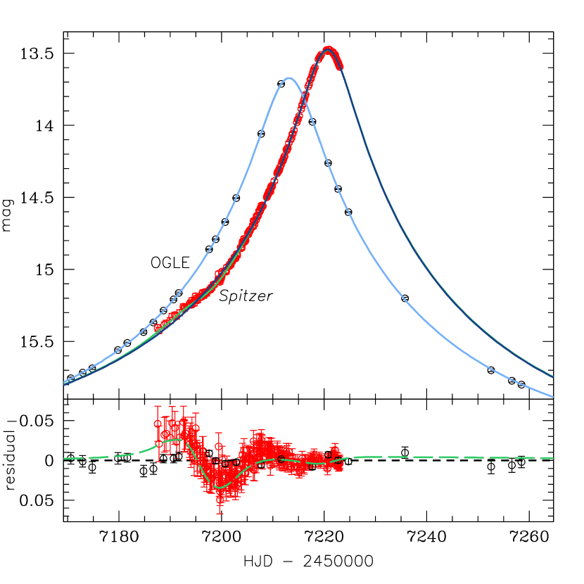
Figure 2.— Point-lens fit (with parallax) to Spitzer and OGLE light curves of OGLE-2015-BLG-0448. The model (light blue line) fits the OGLE data (black points) quite well, but there are strong residuals in the Spitzer data (red points and dark blue line), particularly near the start of the observations. The green line shows the planetary lens model for the Spitzer data, which is discussed in Appendix A. The green long-dashed line in the lower plot shows the difference between the Spitzer point-lens and double-lens models.

The Spitzer residuals are qualitatively similar to those analyzed by Gaudi et al. (2002) for OGLE-1999-BUL-36. They found that this form of residuals could be explained either by a low mass-ratio companion ($q\ll 1$) with projected separation (normalized to $\theta_{\rm E}$) $s<1$, or by light curve distortions induced by the accelerated motion of the observer on Earth, i.e., orbital parallax (Gould, 1992). However, in the present case, the latter explanation is ruled out because the parallax is measured (and already incorporated into the fit) from the offsets in the observed $(t_{0},u_{0})$ as seen from Earth and Spitzer,

$${\mbox{\boldmath$\pi$}}_{{\rm E},\pm\pm}\simeq{{\rm AU}\over D_{\perp}}(\Delta\tau,\Delta\beta_{\pm\pm});$$

$$\qquad\Delta\tau\equiv{t_{0,\oplus}-t_{0,\rm sat}\over t_{\rm E}};\\$$ (3)

$$\qquad\Delta\beta_{\pm\pm}\equiv\pm u_{0,\oplus}-\pm u_{0,\rm sat}.$$

Here, ${\bf D}_{\perp}$ is the Earth-satellite separation projected on the sky (changes from $0.84$ to $1.31~{}{\rm AU}$ over the course of Spitzer observations) and where the subscripts $\oplus$ and “sat” indicate parameters as measured from Earth and the satellite, respectively. The four solutions are specified $(\pm\pm)$ according to the signs of $u_{0}$ as seen from Earth and Spitzer respectively. See Gould (2004) for sign conventions. Table 7 lists four possible solutions, including the heliocentric projected velocity,

$$\tilde{\bf v}_{\rm hel}=\tilde{\bf v}_{\rm geo}+{\bf v}_{\oplus,\perp};\qquad\tilde{\bf v}_{\rm geo}={{\mbox{\boldmath$\pi$}}_{\rm E}\over\pi_{\rm E}^{2}}\,{{\rm AU}\over t_{\rm E}},$$ (4)

where ${\bf v}_{\oplus,\perp}(N,E)=(-0.6,28.3)\,{\rm km}\,{\rm s}^{-1}$ is the velocity of Earth projected on the sky at the peak of the event. The $(-+)$ solution is preferred over the other ones by $\Delta\chi^{2}=6.7$ because OGLE data prefer $\pi_{{\rm E},N}>0$ and this solution has the highest $\pi_{{\rm E},N}$. The comparison of Tables 3 and 7 shows that the OGLE parallax measurement (that is based on slight light curve distortion) is consistent with the OGLE+Spitzer result (that is based on the difference in $t_{0}$ and $u_{0}$ between the two observatories). Figure 3 displays the projected velocity vectors for these four solutions.

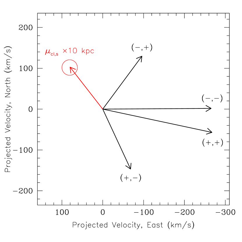
Figure 3.— Comparison of directions of astrometrically measured ${\mbox{\boldmath$\mu$}}_{s,cl}$ (red) with four degenerate projected velocities $\tilde{\bf v}_{\rm hel}$ based on microlensing data. The proper motion measurement has been scaled by an arbitrary distance (10 kpc) so that it has the same units and approximately same size as the projected velocities. The direction of ${\mbox{\boldmath$\mu$}}_{s,cl}$ is inconsistent with any of the four $\tilde{\bf v}_{\rm hel}$. Hence, the lens does not belong to the cluster.

Table 1 OGLE-2015-BLG-0448 Point-Lens Parameters based on OGLE data

Parameter	Unit	$u_{0}>0$	$u_{0}<0$
$\chi^{2}$		$125.1$	$125.0$
$t_{0}$	day	$7213.153$	$7213.153$
		$\pm 0.016$	$\pm 0.016$
$u_{0}$		$0.0874$	$-0.0876$
		$\pm 0.0016$	$\pm 0.0017$
$t_{\rm E}$	day	$61.23$	$60.83$
		$\pm 0.84$	$\pm 0.95$
$\pi_{{\rm E},N}$		$0.113$	$0.180$
		$\pm 0.052$	$\pm 0.081$
$\pi_{{\rm E},E}$		$-0.104$	$-0.111$
		$\pm 0.034$	$\pm 0.037$
$(F_{b}/F_{\rm base})_{\rm OGLE}$		$-0.002$	$-0.004$
		$\pm 0.019$	$\pm 0.020$

There are only three possible causes of Spitzer point-source point-lens residuals: a binary (or planetary) companion to the lens, a binary companion to the source, or an unmodeled systematics in the light curve. Binary-source explanations for the residuals are basically ruled out by the fact that no sign of source binarity is seen in the OGLE light curve. Of course, one possible explanation for the lack of binarity effects would be an extremely red source, which has so much less flux in $I$-band than in Spitzer’s $3.6\mu$m that it simply does not show up in the OGLE data. However, the source is a red giant, so there are very few stars on the color-magnitude diagram (CMD) that are significantly redder. For two of the solutions ($++$ and $--$) in Table 7, the source follows the same trajectory as seen from Earth and Spitzer, just separated in time. Hence, binary-source solutions are obviously inconsistent with the OGLE data. For the other two solutions, the second source could pass farther from the lens as seen from Earth compared to the Spitzer by a factor $\approx 1+(u_{0,\rm sat}+u_{0,\oplus})/u_{0,\rm sat^{\prime}}\approx 1+0.16/u_{0,\rm sat^{\prime}}$ where $u_{0,\rm sat^{\prime}}$ is the impact parameter of the source’s companion as seen by the Spitzer. Given the slow development of the deviation, $u_{0,\rm sat^{\prime}}\gtrsim 0.1$, implying that this ratio of impact parameters is $\lesssim 2.6$. The source is already close to the reddest stars on the CMD, hence, the amplitudes of deviation have to be similar to the ratio of impact parameters, which is clearly ruled out by the data. Notwithstanding these general arguments, we fit for binary-source solutions. We confirm that they are not viable. The binary lens models with planetary mass ratio are discussed in Appendix A.

4. Proper Motion Measurements

4.1. NGC 6558 Proper Motion Measurements in Literature

The first measurement of the NGC 6558 proper motion was presented by Vásquez et al. (2013). Stars on the upper red giant branch ($I<16.5\,{\rm mag}$) and bluer than bulge giants were selected as cluster members and the mean proper motion of these stars was reported: ${\mbox{\boldmath$\mu$}}_{cl}(N,E)=(0.06\pm 0.14,0.52\pm 0.14)\,{\rm mas}\,{\rm yr}^{-1}$. The bluer red giants were chosen because the metallicity of the cluster stars is lower than the bulge red giants. Hence, cluster members on the giant branch are expected to be bluer. However, the bulge red giants show significant metallicity spread (Zoccali et al., 2008) and thus some bulge red giants can be mistaken for cluster members. Therefore, one expects the Vásquez et al. (2013) measurement to be biased toward smaller proper motion values. Additionally, the cluster proper motion relative to the bulge could be underestimated because cluster members may have been included in the ensemble used to establish the “bulge” frame.

Rossi et al. (2015) published the only other NGC 6558 proper motion: ${\mbox{\boldmath$\mu$}}_{cl}(N,E)=(0.47\pm 0.60,-0.12\pm 0.55)\,{\rm mas}\,{\rm yr}^{-1}$. In their approach cluster member selection and frame alignment (needed for any proper motion measurement) were combined into one iterative process. The CMD decomposed into cluster and field stars can be used to diagnose the reliability of this process. The most prominent cluster feature on the CMD is the blue horizontal branch defined by the stars of $V>16$ and $(V-I)<0.9$. The decomposed CMDs for the cluster and the field reveal a very similar number of stars in this region, even though we do not expect field stars with these properties. The problems with decomposing blue horizontal branch stars suggests that the iterative process used to select cluster members and measure proper motions, failed in this case.

4.2. NGC 6558 Proper Motion Measurement From OGLE-IV Data

We use two different methods to measure the proper motion of NGC 6558. In both cases, we make use of 5 years of OGLE-IV observations of this field. We first establish a “Galactic bulge reference frame” by identifying red giant stars from the CMD on the chip where the cluster lies, but excluding a circle of radius $1\farcm 52$ around the cluster itself. We note that for the immediate purpose of this paper, it is not important whether this reference frame is contaminated by non-bulge stars because we will measure the proper motion of the source in the same frame. However, the general utility of this measurement does require that this be the bulge frame, and the red giants are the best way to define this. Because the reference frame is defined by 2000 stars whose dispersion is about $2.7\,{\rm mas}\,{\rm yr}^{-1}$ in each direction, it is randomly offset from the “true bulge frame” by $0.06\,{\rm mas}\,{\rm yr}^{-1}$ in each direction.

In the first method, we measure the proper motion of each star $I<18\,{\rm mag}$ within a radius of $0\farcm 87$ from the cluster center. We fit the resulting distribution of 518 proper motion measurements to the sum of two two-dimensional Gaussians, described by a total of four parameters, i.e., the cluster proper motion ${\mbox{\boldmath$\mu$}}_{cl}$, a single isotropic “cluster” dispersion $\sigma_{cl}$ (actually mostly due to measurement error rather than intrinsic dispersion), and the fraction of all stars in the sample that belong to the cluster, $p$. The second Gaussian is assumed to have the same properties as the bulge population, i.e, a centroid at $(0,0)$ and a dispersion $(2.7,2.7)\,{\rm mas}\,{\rm yr}^{-1}$.

We find $p=24\pm 3\%$, $\sigma_{cl}=0.65\,{\rm mas}\,{\rm yr}^{-1}$, and

$${\mbox{\boldmath$\mu$}}_{cl,1}(N,E)=(+0.36\pm 0.08,+1.39\pm 0.08)\,{\rm mas}\,{\rm yr}^{-1}.$$ (5)

See Figure 4.

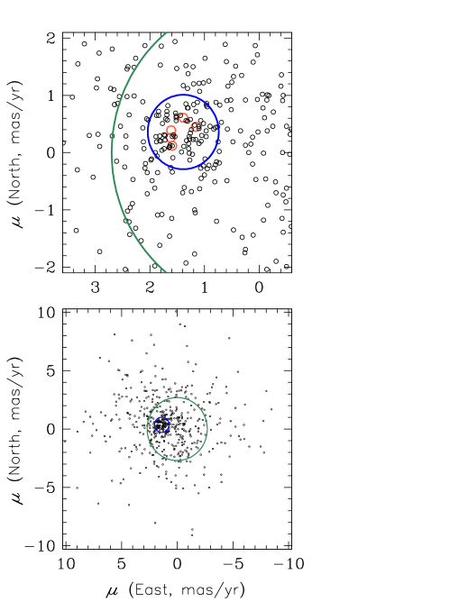
Figure 4.— Proper motions of stars within $0\farcm 87$ of the center of NGC 6558 based on OGLE-IV data. The distribution was fit to the sum of two Gaussians, one for the bulge, centered at (0,0) and with the known bulge dispersion $\sigma=2.7\,{\rm mas}\,{\rm yr}^{-1}$ (green circle), and the other with freely fit center and dispersion (blue circle). This gives one measure of the cluster proper motion in the bulge frame ${\mbox{\boldmath$\mu$}}_{cl}(N,E)=(+0.36\pm 0.08,+1.39\pm 0.08)$. In a second method, we take the average proper motion of five spectroscopically confirmed cluster members (small red circles, upper zoomed panel only), which yields ${\mbox{\boldmath$\mu$}}_{cl}(N,E)=(+0.33\pm 0.08,+1.49\pm 0.08)$. Since these are consistent, we combine them to yield Equation (7).

In the second method, we measure the proper motions of five spectroscopically confirmed cluster members (Zoccali et al., 2008; Dias et al., 2015), and find

$${\mbox{\boldmath$\mu$}}_{cl,2}(N,E)=(+0.37\pm 0.08,+1.47\pm 0.09)\,{\rm mas}\,{\rm yr}^{-1},$$ (6)

where the error is determined from the scatter. See the upper panel of Figure 4. Since these are consistent at the $1\,\sigma$, we combine the two measurements to obtain

$${\mbox{\boldmath$\mu$}}_{cl}(N,E)=(+0.36\pm 0.06,+1.42\pm 0.06)\,{\rm mas}\,{\rm yr}^{-1}.$$ (7)

We remind the reader that these errors are relative to the frame, which is what is relevant to our current application. Since the frame itself has errors of $0.06\,{\rm mas}\,{\rm yr}^{-1}$, the total error in this value in the “true bulge frame” is $0.08\,{\rm mas}\,{\rm yr}^{-1}$.

4.3. Proper Motion of Source Star

We measure the proper motion of the OGLE-2015-BLG-0448 source in the same frame:

$${\mbox{\boldmath$\mu$}}_{s}(N,E)=(-1.81\pm 0.40,-0.27\pm 0.40)\,{\rm mas}\,{\rm yr}^{-1}.$$ (8)

We estimate the error in two ways. First, we note that the two methods of measuring ${\mbox{\boldmath$\mu$}}_{cl}$ revealed scatters of $0.65\,{\rm mas}\,{\rm yr}^{-1}$ and $0.18\,{\rm mas}\,{\rm yr}^{-1}$ for the two star samples with median brightness of $I\approx 17.2\,{\rm mag}$ and $I\approx 14.2\,{\rm mag}$, respectively. Given that the OGLE-2015-BLG-0448 source has a baseline magnitude of $I_{\rm base}=16.34$, we adopt an intermediate value of $0.40\,{\rm mas}\,{\rm yr}^{-1}$. Second, substantial experience from regions where two OGLE fields overlap, shows that proper-motion errors are typically at about this level for $I\approx 16.5\,{\rm mag}$ stars.

The relative proper motion between the cluster and the source-star is

$${\mbox{\boldmath$\mu$}}_{cl,s}(N,E)=(+2.17\pm 0.40,+1.69\pm 0.40)\,{\rm mas}\,{\rm yr}^{-1}.$$ (9)

4.4. Lens Is Not Cluster Member

We put the proper motion vector ${\mbox{\boldmath$\mu$}}_{cl,s}$ (Equation (9)) on Figure 3 in order to test whether its direction is consistent with any of the lens-source projected velocities. Because ${\mbox{\boldmath$\mu$}}_{cl,s}$ and $\tilde{\bf v}_{\rm hel}$ have different units, ${\mbox{\boldmath$\mu$}}_{cl,s}$ must be multiplied by a dimensional quantity in order to be displayed on the same plot. We call this $D_{\rm rel}$ for reasons that will become clear. We have chosen $D_{\rm rel}=10\,{\rm kpc}$ simply because the vectors are then roughly the same size. The ${\mbox{\boldmath$\mu$}}_{cl,s}$ is clearly inconsistent with any of the four values of $\tilde{\bf v}_{\rm hel}$, hence the lens is definitely not in the cluster.

However, if ${\mbox{\boldmath$\mu$}}_{cl,s}$ had been consistent with one of the $\tilde{\bf v}_{\rm hel}$, then the $D_{\rm rel}$ required to make the two vectors in Figure 3 align would have provided an additional test for cluster membership. That is,

$${\tilde{v}_{\rm hel}\over\mu_{l,s}}={{\rm AU}\over\pi_{\rm rel}}\rightarrow D_{\rm rel},$$ (10)

where ${\mbox{\boldmath$\mu$}}_{l,s}$ is the lens-source relative proper motion, which for our purposes can be taken as identical to the cluster proper motion, because $|\mu_{l,s}-\mu_{cl,s}|\leq|{\mbox{\boldmath$\mu$}}_{l}-{\mbox{\boldmath$\mu$}}_{cl}|=v_{l,cl}/D_{L}\lesssim 0.2\,{\rm mas}\,{\rm yr}^{-1}$. Here ${\bf v}_{l,cl}$ is the lens velocity in the cluster frame.

If, for example, ${\mbox{\boldmath$\mu$}}_{cl,s}$ had been in exactly the opposite direction to the one measured, it would have been consistent in direction with $\tilde{\bf v}_{{\rm hel},+-}$. Then, identifying the lens as in the cluster would have implied $\pi_{{\rm rel},cl,s}\simeq 100\,{\mu\rm as}$. This would have been an implausible value because the cluster is believed to be at $D\approx 7\,{\rm kpc}$, i.e, $\pi_{cl}\approx 140\,{\mu\rm as}$, which would imply $\pi_{s}=40\,{\mu\rm as}$, i.e., $D_{L}=25\,{\rm kpc}$. That is, the $D_{\rm rel}$ required to align ${\mbox{\boldmath$\mu$}}_{cl,s}$ and $\tilde{\bf v}_{\rm hel}$ provides a powerful consistency check on the identification of the lens as a cluster member.

5. Location of Lensing System

For a large fraction of past planetary microlensing events, $\theta_{\rm E}$ is measured from the finite source effects, since the model then yields $\rho=\theta_{*}/\theta_{\rm E}$ and the angular source radius $\theta_{*}$ is easily measured (Yoo et al., 2004). Unfortunately, this event contains no caustic crossings or cusp approaches so this standard method cannot be applied. Calchi Novati et al. (2015a) showed that for events with measured parallaxes ${\mbox{\boldmath$\pi$}}_{\rm E}$, the lens distance (and hence the mass) could be estimated kinematically, with relatively small error bars. However, of the 21 events analyzed there, all but one had projected velocities that either were quite large $\tilde{v}_{\rm hel}>700\,{\rm km}\,{\rm s}^{-1}$ or were consistent in direction with Galactic rotation. The first group are easily explained as Galactic bulge lenses $\pi_{\rm rel}\lesssim 0.02\,{\rm mas}$, since $\mu=\tilde{v}_{\rm hel}\pi_{\rm rel}/{\rm AU}=3\,{\rm mas}\,{\rm yr}^{-1}(\tilde{v}/700\,{\rm km}\,{\rm s}^{-1})(\pi_{\rm rel}/0.02\,{\rm mas})$, which is a typical value for bulge lenses. The second group are easily explained as lenses rotating with the Galactic disk, with the magnitude of $\tilde{v}_{\rm hel}$ giving a rough kinematic distance estimate $\pi_{\rm rel}\simeq\mu_{sgrA*}{\rm AU}/\tilde{v}_{\rm hel}$ and $\mu_{sgrA*}=6.38\,{\rm mas}\,{\rm yr}^{-1}$ is the proper motion of SgrA*. The one exception was OGLE-2014-BLG-0807, for which the favored solutions had $\tilde{v}_{\rm hel}\approx 200\,{\rm km}\,{\rm s}^{-1}$.

The best model $(-+)$ in Table 7 has $\tilde{v}_{\rm hel}=161.2(4)\,{\rm km}\,{\rm s}^{-1}$, while the models $(++)$ and $(--)$ that fit the data slightly worse, predict $\tilde{v}_{\rm hel}=270\,{\rm km}\,{\rm s}^{-1}$. Neither of the $\tilde{\bf v}_{\rm hel}$ vectors is aligned with Galactic disk rotation, hence there is a low probability that the lens is in the Galactic disk. The measured projected velocity could be explained by a bulge lens if the lens-source relative parallax were larger than typical. The line of sight toward the event at Galactic coordinates $(l,b)=(0\fdg 20,\,-6\fdg 01)$ crosses the two arms of the bulge X-shaped structure (Nataf et al., 2010; McWilliam & Zoccali, 2010; Gonzalez et al., 2015). Hence, it is possible that the lens is in the closer part of the bulge and the source is much further away and the relative parallax is higher than typical. Even in this case the $\tilde{v}_{\rm hel}=270\,{\rm km}\,{\rm s}^{-1}$ solutions would be preferred over $\tilde{v}_{\rm hel}=160\,{\rm km}\,{\rm s}^{-1}$, i.e., contrary to the least-squares fits to the OGLE data. In either case, the most probable lens location is in the closer part of the bulge.

6. Planet Sensitivity

With peak magnifications of 11 (from ground) and 14 (from Spitzer), and average cadences of 36 per day (ground-based survey plus follow-ups) and 6 per day (for Spitzer), event OGLE-2015-BLG-0448 is among the Spitzer 2015 events that are most sensitive to planet perturbations. Therefore, we present the planet sensitivity of this event here, it will also be required for the determination of the Galactic distribution of planets, no matter whether the planet detection in this event is real or not.

We compute the planet sensitivity of this event using the method that was first proposed by Rhie et al. (2000) and further developed by Yee et al. (2015) and Zhu et al. (2015) to include space-based observations. Details of the method can be found in the latter two references. In brief, we first measure the planet sensitivity $S$ as a function of $q$ and $s$. For each set of $(q,s)$, we generate 300 planetary light curves that vary in angle between the source trajectory and the lens binary axis, $\alpha$, but have other parameters fixed to the observed values. For each simulated light curve, we then find the best-fit single-lens model using the downhill simplex algorithm. The deviation between the simulated data and its best-fit single-lens model is quantified by $\chi^{2}_{\rm SL}$. For a subjectively chosen event, which is the case of OGLE-2015-BLG-0448, we first fit the simulated data that were released before the selection date $t_{\rm select}$ and find $\chi^{2}_{\rm SL,select}$. If $\chi^{2}_{\rm SL,select}>10$, we regard the injected planet as having been noticeable and thus reject this $\alpha$; otherwise we compare $\chi^{2}_{\rm SL}$ from the whole light curve with our pre-determined detection threshold, and consider the injected planet as detectable if $\chi^{2}_{\rm SL}>\chi^{2}_{\rm threshold}$. The sensitivity $S(q,s)$ is the fraction of $\alpha$ values for which the planet is detectable. We assume Öpik’s law in $s$, i.e., a flat distribution of $\log{s}$, and compute the integrated planet sensitivity $S(q)$.

We adopt the following detection thresholds, which are more realistic than that used in Zhu et al. (2015): C1: $\chi^{2}_{\rm SL}>300$ and at least three consecutive data points showing $>3~{}\sigma$ deviations; or C2: $\chi^{2}_{\rm SL}>500$. C1 is used mainly to recognize sharp planetary anomalies. Some of these anomalies might not be treated as reliable detections with only the current data, because of the low $\chi^{2}_{\rm SL}$. However, they are nevertheless significant enough to trigger the automatic anomaly detection software and/or attract human attentions, either of which would lead to dedicated follow-up observations of the anomalies and thus confirm these otherwise marginal detections. C2 as a supplement of C1 intends to capture the long-term weak distortions that may not show sharp deviations.

The calculation of planet sensitivity requires $\rho$ as an input. Here we estimate $\rho$ following the prescription given by Yee et al. (2015): $\rho=\theta_{*}/\theta_{\rm E}$ where $\theta_{\rm E}=\pi_{\rm rel}/\pi_{\rm E}$. The parallax $\pi_{\rm E}$ is well measured thanks to a combination of the OGLE and the Spitzer data, hence below we need to estimate only $\pi_{\rm rel}$ and $\theta_{*}$. The lens-source relative parallax can be easily found under the assumption that the lens is in the closer arm of the X-shaped structure and the source is in the further arm. We follow Nataf et al. (2015) who in detail modeled properties of the X-shaped structure in OGLE-III fields. The two centroids of RC luminosity functions corrected for extinction are $I_{{\rm RC}1,0}=14.210~{}{\rm mag}$ and $I_{{\rm RC}2,0}=14.715~{}{\rm mag}$ for the event location (average values for fields BLG169 and BLG170). For absolute RC brightness of $M_{I,{\rm RC}}=-0.12~{}{\rm mag}$ the corresponding distances are $7.3$ and $9.3~{}{\rm kpc}$, hence, $\pi_{\rm rel}=0.028~{}{\rm mas}$.

To calculate $\theta_{*}$ we assume the source $I$-band brightness and $(V-I)$ color are the same as the baseline object: $I_{s}=16.337~{}{\rm mag}$ and $(V-I)_{s}=1.589~{}{\rm mag}$ (Szymański et al., 2011). This is justified because none of our models predicts significant blending. We corrected for extinction using Nataf et al. (2013) extinction maps and obtain: $I_{s,0}=15.711~{}{\rm mag}$ and $(V-I)_{s,0}=1.046~{}{\rm mag}$. This $(V-I)_{s,0}$ corresponds to $(V-K)_{s,0}=2.419~{}{\rm mag}$ (Bessell & Brett, 1988). The Kervella et al. (2004) color-surface brightness relation gives $\theta_{*}=3.4~{}{\rm\mu as}$. Finally, $\rho=\theta_{*}\pi_{\rm E}/\pi_{\rm rel}=0.019$ and $0.011$ for $(-+)$ and $(--)$ models, respectively.

We plot all the ground-based data in Figure 5. The highest contribution to the planet sensitivity comes from the Auckland and LCOGT CTIO A datasets. We compute the planet sensitivity for two out of four possible solutions, $(--)$ and $(-+)$, and show the results in Figure 6. Both solutions show substantial planet sensitivity ($>10\%$) down to $q=10^{-4}$. The $(-+)$ solution shows slightly higher sensitivity for $q\gtrsim 2\times 10^{-4}$, mostly because observations taken from the satellite and Earth are probing different regions in the Einstein ring, as has been discussed in Zhu et al. (2015) and the reader can also see Figure 7 here for a demonstration. At smallest $q$ values the $(-+)$ solution is less sensitive than the $(--)$ solution, because the larger source size ($\rho=0.019$) smears out subtle features due to small planets. Figure 7 shows the detectability of planets with mass ratio $q=1.70\times 10^{-4}$ as functions of planet positions for both investigated solutions. It is clear that the tentative planet detection reported here can only happen in the $(-+)$ solution.

7. Conclusions

The event OGLE-2015-BLG-0448 presented a number of unique properties. It lay projected within tidal radius of the globular cluster. The maximum magnification reached was relatively high both for Spitzer and ground-based observations. It was also intensively monitored both from the ground and from space. All these properties made it a potential probe of the population of planets in globular clusters.

We analyzed the event photometry from both Spitzer and ground-based telescopes: the OGLE survey and follow-up networks of $\mu$FUN, RoboNet, and MiNDSTEp. Microlens parallax was measured using the difference in event properties as seen from ground and space. The result confirmed the microlens parallax measured using only the OGLE data. Additionally, long-term astrometry of OGLE images was used to measure proper motions. We measured the proper motion of globular cluster NGC 6558 and the event source. Our analysis reveals that the lens could not be a cluster member. The same methods can be used for other potential cluster lens events that are observed by satellites.

We found that the Spitzer light curve reveals significant trends in residuals of the point-source point-lens model. The only two plausible causes of these trends are problems with Spitzer photometry or a planetary companion to the lens. We do not claim planet detection, but provide results of planetary model fitting in case the event photometry is proven correct.

Appendix A Tentative Planet

The point source model fitted to the Spitzer data resulted in residuals with significant trends. Here we discuss the possibility that these residuals were caused by the companion to the lens.

The only possible binary-lens solutions must have planetary mass ratios $q\ll 1$ and separations satisfying $|s-s^{-1}|\approx 0.5$, i.e., $\log s\approx\pm 0.11$, which follows from simple arguments. First, the source passes the lens at $u_{0}\approx 0.08$ as seen from both Earth and Spitzer. Since neither light curve is perturbed at peak, this already implies that the central caustic is small. Such small central caustics require either $s\ll 1$, $s\gg 1$, and/or $q\ll 1$. However, if either of the first two held, there could not be a significant perturbation at the point that it is observed at $u_{\rm sat}\approx 0.5$. That is, the event timescale $t_{\rm E}\approx 60\,$days is set by the unperturbed OGLE light curve. Hence, the fact that the Spitzer curve experiences an excess roughly 30 days before peak implies that there is a caustic structure at $u_{\rm sat}\approx 30/60=0.5$.

Thus, $q\ll 1$. In this planetary regime, such caustics occur when the planet is aligned to one of the two unperturbed images of the primary lens at $u=|s-s^{-1}|$, i.e., $s=|-u\pm(u^{2}+4)^{1/2}|/2$. Hence, $|\log s|\approx 0.11$.

Finally, the fact that the Spitzer light curve is perturbed while the OGLE light curve is not, implies (as in the above binary source analysis), that the source passes on opposite sides of the lens ($+-$ or $-+$ solutions). The preference of $(-+)$ in Table 7 makes it the best solution.

We consider four different topologies obeying the above constraints. First, $s<1$ with the source (seen by Spitzer) passing between the two triangular caustics for this topology. Second, $s<1$ with the source passing outside one of these caustics. Third, $s>1$. For each topology, we insert a series of seed solutions as a function of $q$ and allow all parameters to vary. We find that the first and the third topologies never match the observed morphology of the Spitzer light curve because their relative demagnification zones do not align to the relative “dip” in the Spitzer light curve at about ${\rm HJD}^{\prime}=7200$. The second topology always converges to the same solution, which we present in Figure 8. The model Spitzer light curve is shown in Figure 2 by green line. The single lens parameters are consistent with the $(-+)$ solution in Table 7: $t_{0}=7213.161(14)$, $u_{0}=-0.0870(10)$, $t_{\rm E}=61.16(16)\,{\rm d}$, $\pi_{{\rm E},N}=0.1140(12)$, $\pi_{{\rm E},E}=-0.1088(10)$, and $F_{b}/F_{\rm base,OGLE}=0.002(11)$. The additional binary lens parameters are: $\alpha=189\fdg 71(25)$, $s=0.7870(50)$, and $q=1.70(32)\times 10^{-4}$. The $\chi^{2}/dof=209.7/331$ is better by $\chi^{2}=127.7$ than the point-lens solution, and better by $\Delta\chi^{2}=49$ than the double-lens $(+-)$ solution. We note that even the best-fitting model does not remove all the systematics seen in Spitzer residuals.

The light curve lacks close approach to the caustics, which is uncommon among published microlensing planets (Zhu et al., 2014). Without the caustic approach we are unable to constrain the source size relative to $\theta_{\rm E}$. We note that Yee et al. (2013) found a planetary signal below the reliability threshold in MOA-2010-BLG-311 event that also lies close to a globular cluster (NGC 6553 in that case).

Table 2 OGLE-2015-BLG-0448 Point-Lens Parameters based on OGLE and Spitzer data

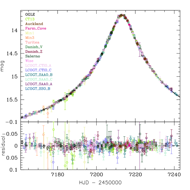
Figure 5.— Ground-based light curve of OGLE-2015-BLG-0448. Different colors represent different datasets. For clarity, the follow-up data were averaged in bins separately chosen for each dataset. The bins were set based on comparison of the uncertainty of the mean point and the change of the model brightness over the bin timespan. For each bin the uncertainty of the mean point is smaller than the maximum difference between the model brightness and the mean model value. There are 462 bins that are based on 1638 follow-up data points.

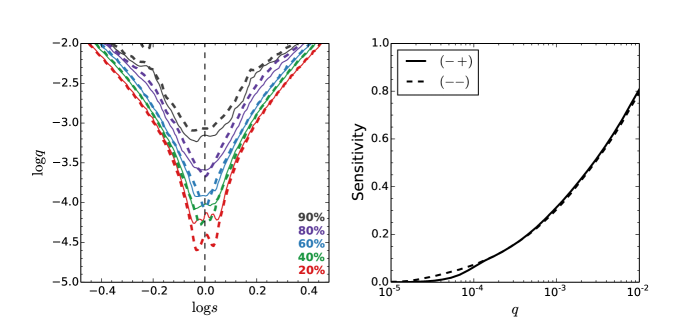
Figure 6.— Planet sensitivity results of OGLE-2015-BLG-0448. The sensitivity as a function of two parameters, $S(q,s)$, is shown on the left panel, and on the right is shown the integrated sensitivity $S(q)$ when a flat distribution of $s$ in $\log{s}$ is assumed. In both panels we show the sensitivities of two solutions $(-+)$ (solid) and $(--)$ (dashed).

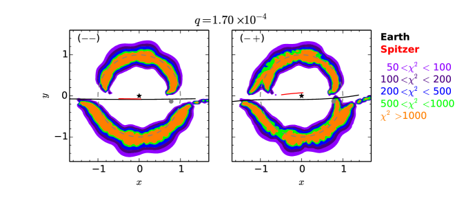
Figure 7.— The $\chi^{2}$ distributions of simulated OGLE-2015-BLG-0448 light curves with a $q=1.7\times 10^{-4}$ planet placed at different positions $(x,y)$. The left panel shows the result for the $(--)$ solution, and the right panel shows that for the $(-+)$ solution. The black/red lines indicate the source trajectories as seen from Earth/Spitzer. The lens is placed at $(0,0)$, and the position of the tentative planet is shown as a filled gray dot. Note that the tentative planet could only be detected in the $(-+)$ solution.

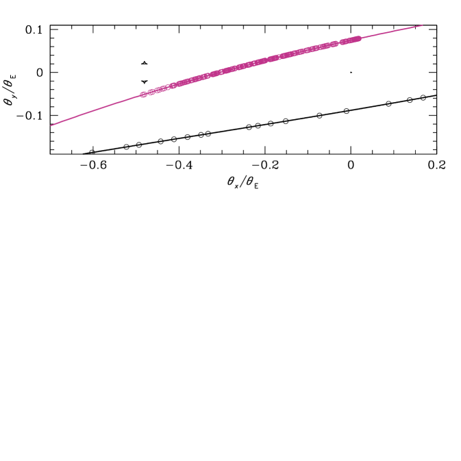
Figure 8.— Source trajectory as seen from Spitzer (violet) and Earth (black). The central caustic is located at $(\theta_{x},\theta_{y})=(0,0)$ and two triangular planetary caustics are at $\theta_{x}/\theta_{\rm E}=s-1/s\approx-0.48$. The circles indicate apparent source positions at the epoch when Spitzer and OGLE data were taken.

References

- Bessell & Brett (1988) Bessell, M.S., & Brett, J.M. 1988, PASP, 100, 1134
- Bramich (2008) Bramich, D.M. 2008, MNRAS, 386, L77.
- Bramich et al. (2013) Bramich, D.M. et al, 2013, MNRAS, 428, 2275.
- Brown et al. (2013) Brown, T.M., Baliber, N., Bianco, F.B. et al., 2013, PASP, 125, 1031
- Calchi Novati et al. (2015a) Calchi Novati, S., Gould, A., Udalski, A., et al., 2015a, ApJ, 804, 20
- Calchi Novati et al. (2015b) Calchi Novati, S., Gould, A., Yee, J.C., et al., 2015b, ApJ, 814, 92
- Dias et al. (2015) Dias, B., Barbuy, B., Saviane, I., et al. 2015, A&A, 573, 13
- Dominik et al. (2008) Dominik, M., Horne, K., Allan, A., et al. 2008, AN, 329, 248
- Dominik et al. (2010) Dominik, M., Jørgensen, U.G., Rattenbury, N.J., et al. 2010, AN, 331, 671
- Gaudi et al. (2002) Gaudi, B.S., Albrow, M.D., An, J., et al. 2002, ApJ, 566, 463
- Gonzalez et al. (2015) Gonzalez, O.A., Zoccali, M., Debattista, V.P., Alonso-García, J., Valenti, E. & Minniti, D. 2015, A&A, 583, L5
- Gould (1992) Gould, A. 1992, ApJ, 392, 442
- Gould (1994) Gould, A. 1994, ApJ, 421, L75
- Gould (2004) Gould, A. 2004, ApJ, 606, 319
- Gould et al. (2014) Gould, A., Carey, S., & Yee, J. Galactic Distribution of Planets from Spitzer Microlens Parallaxes Spitzer Proposal ID#11006
- Gould & Horne (2013) Gould, A. & Horne, K. 2013, ApJ, 779, 28
- Gould & Loeb (1992) Gould, A. & Loeb, A. 1992, ApJ, 396, 104
- Griest & Safizadeh (1998) Griest, K. & Safizadeh, N. 1998, ApJ, 500, 37
- Harris (1996) Harris, W.E 1996, AJ, 112, 1487
- Hundertmark et al. (2015) Hundertmark, M.P.G. et al., 2015, in prep.
- Kervella et al. (2004) Kervella, P., Bersier, D., Mourard, D. et al. 2004, A&A, 428, 587
- Kunder et al. (2008) Kunder, A., Popowski, P., Cook, K.H., & Chaboyer, B. 2008, AJ, 135, 631
- Mao & Paczyński (1991) Mao, S., & Paczyński B. 1991, ApJ, 374, L37
- McWilliam & Zoccali (2010) McWilliam, A., & Zoccali, M. 2010, ApJ, 724, 1491
- Nascimbeni et al. (2012) Nascimbeni, V., Bedin, L.R., Piotto, G., De Marchi, F., & Rich, R.M. 2012, A&A, 541, 144
- Nataf et al. (2010) Nataf, D.M., Udalski, A., Gould, A., Fouqué, P., & Stanek, K.Z. 2010, ApJ, 721, L28
- Nataf et al. (2013) Nataf, D.M., Gould, A., Fouqué, P. et al. 2013, ApJ, 769, 88
- Nataf et al. (2015) Nataf, D.M., Udalski, A., Skowron, J. et al. 2015, MNRAS, 447, 1535
- Paczyński (1986) Paczyński, B. 1986, ApJ, 304, 1
- Paczyński (1994) Paczyński, B. 1994, Acta Astron., 44, 235
- Refsdal (1966) Refsdal, S. 1966, MNRAS, 134, 315
- Refsdal (1964) Refsdal, S. 1964, MNRAS, 128, 295
- Rhie et al. (2000) Rhie, S.H., Bennett, D.P., Becker, A.C., et al. 2000, ApJ, 533, 378
- Richer et al. (2003) Richer, H.B., Ibata, R., Fahlman, G.G., & Huber, M. 2003, ApJ, 597, 45
- Rossi et al. (2015) Rossi, L.J., Ortolani, S., Barbuy, B., Bica, E., & Bonfanti, A. 2015, MNRAS, 450, 3270
- Schechter et al. (1993) Schechter, P.L., Mateo, M., & Saha, A. 1993, PASP, 105, 1342
- Skottfelt et al. (2015) Skottfelt, J., Bramich, D. M., Hundertmark, M., et al. 2015, A&A, 574, A54
- Smith et al. (2003) Smith, M., Mao, S., & Paczyński, B. 2003, MNRAS, 339, 925
- Soszyński et al. (2011) Soszyński, I., Dziembowski, W.A., Udalski, A., et al. 2011, Acta Astron., 61, 1
- Szymański et al. (2011) Szymanński, M.K., Udalski, A., Soszyński., I., et al. 2011, Acta Astron., 61, 83
- Swift et al. (2015) Swift, J.J., Bottom, M., Johnson, J.A., et al. 2015, JATIS, 1, 2
- Udalski (2003) Udalski, A. 2003, Acta Astron., 53, 291
- Udalski et al. (2015) Udalski, A., Szymański, M.K. & Szymański, G. 2015, Acta Astron., 65, 1
- Udalski et al. (1994) Udalski, A., Szymański, M., Kałużny, J., Kubiak, M., Mateo, M., Krzemiński, W., & Paczyński, B. 1994, Acta Astron., 44, 317
- Vásquez et al. (2013) Vásquez, S., Zoccali, M., Hill, V., et al. 2013, A&A, 444, 91
- Yee et al. (2013) Yee, J.C., Hung, L.-W., Bond, I.A., et al. 2013, ApJ, 769, 77
- Yee et al. (2015) Yee, J.C., Gould, A., Beichman, C., et al. 2015, ApJ, 810, 155
- Yoo et al. (2004) Yoo, J., DePoy, D.L., Gal-Yam, A. et al. 2004, ApJ, 603, 139
- Zhu et al. (2014) Zhu, W., Penny, M., Mao, S., Gould, A., & Gendron, R. 2014, ApJ, 788, 73
- Zhu et al. (2015) Zhu, W., Gould, A., Beichman, C., et al. 2015, ApJ, 814, 129
- Zoccali et al. (2008) Zoccali, M., Hill, V., Lecureur, A., et al. 2008, A&A, 486, 177Z