Abstract

The use of effective local Coulomb interactions that are dynamical, that is, frequency-dependent, is an efficient tool to describe the effect of long-range Coulomb interactions and screening thereof in solids. The dynamical character of the interaction introduces the coupling to screening degrees of freedom such as plasmons or particle-hole excitations into the many-body description. We summarize recent progress using these concepts, putting emphasis on dynamical mean field theory (DMFT) calculations with dynamical interactions (“doubly dynamical mean field theory”). We discuss the relation to the combined GW+DMFT method and its simplified version “Screened Exchange DMFT”, as well as the cumulant schemes of many-body perturbation theory. On the example of the simple transition metal SrVO₃, we illustrate the mechanism of the appearance of plasmonic satellite structures in the spectral properties, and discuss implications for the low-energy electronic structure.

1 Theoretical Spectroscopy: from many-body perturbation theory to dynamical Hubbard interactions

Determining the behavior of a single electron in a periodic potential, created for example by the ions in a cristalline solid, is a textbook exercise of quantum mechanics. Determining the wave function of all the electrons in the solid, however, is an intractable many-body problem. The Pauli principle imposes full antisymmetry under exchange of any two electrons to this object, and electronic Coulomb interactions prevent it from being a simple Slater determinant.

The good news is that in practice the knowledge of the full many-body wave function of the inhomogeneous electron gas in the solid is barely necessary: the relevant electronic properties are determined by the low-energy response to external perturbations, and the knowledge of these low-energy excitations requires much less information than the full ground-state wave function. In this sense, solid state spectroscopies are a most efficient means for characterizing the properties of a solid state system. An important example are photoemission experiments – angle-resolved or angle-integrated – where information about the electron removal and addition spectra are obtained. Within the simplest possible model for the photoemission process, the so-called “three-step model”, the photocurrent can be expressed in terms of the one-particle spectral function $A(k,\omega)=-\frac{1}{\pi}Tr\Im G(k,\omega)$, and computing this quantity from first principles, that is, without adjustable parameters, is one of the central challenges of modern theoretical spectroscopy.

Important progress has been achieved over the last decades within many-body perturbation theory: a first order expansion of the many-body self-energy $\Sigma$ in the screened Coulomb interaction $W$ [1, 2] leads to a conceptually simple approximation $\Sigma=iGW$ which can be calculated within realistic electronic structure codes based on density functional theory (DFT). For reviews of successful applications of the GW approximation and developments based on it, we refer the reader to [3, 4]. For more strongly correlated materials, where perturbative techniques reach their limits, the last 15 years have seen the development of a non-perturbative theory, combining dynamical mean field theory (DMFT) [5] with density functional theory. This so-called “DFT+DMFT” approach [6, 7] builds on the success of DMFT for the description of lattice models for correlated fermions but extends its scope to the solid by treating a realistic (multi-orbital) Hamiltonian with effective local Coulomb interaction, often parametrized as Hubbard $U$ and Hund’s $J$.

While DFT+DMFT – at least in its early implementations – can simply be understood as the DMFT solution of a multi-orbital Hubbard model (for reviews see [8, 9, 10], for some more modern implementations [11, 12]) recent efforts have been spent in order to promote DMFT-based techniques to truly first-principles techniques [13]. This implies not only addressing the question of how to relate effective local Hubbard interactions to the full Coulomb interactions in the continuum (while taking care to avoid double-counting of screening), that is the ab initio calculation of the infamous effective local “Hubbard U”; since at the DFT level no rigorous distinction between contributions of “correlated degrees of freedom” and “uncorrelated” ones can be made, a truly double-counting free theory can only be achieved by eliminating the reference to the DFT Kohn-Sham Hamiltonian altogether. A successful route is the combination of Hedin’s GW approximation with DMFT, the so-called GW+DMFT method [14, 15, 16, 17]. A summary of recent progress along these lines can be found in [13]; for most recent applications both, in the model and realistic electronic structure context we refer the reader to Refs. [18, 19, 20, 21, 22]. The common point between the GW method and the combined GW+DMFT scheme is the absence of adjustable interaction parameters. Both theories can be viewed as approximations to a free energy functional [23], where the free energy of the solid is written as a functional of the Green’s function $G$ and the screened Coulomb interaction $W$. This implies that screening is described within the theory, instead of being introduced into it through an effective parameter. Besides the screened Coulomb interaction $W$, the GW+DMFT theory introduces an effective local interaction $\mathcal{U}$ used as the bare interaction within an effective local model. The GW+DMFT equations require this interaction to be calculated self-consistently such as to reproduce the local part of the fully screened interaction $W$ when the local model is solved by many-body techniques. This implies that the two interactions are related by a two-particle Dyson (or Bethe-Salpeter) equation $\mathcal{U}^{-1}-W_{loc}^{-1}=P_{loc}$, where $P_{loc}$ is the polarisation function of the local problem. The physical content of this construction can be described as follows: instead of using the full long-range Coulomb interaction within a full continuum description, an effective local interaction $\mathcal{U}$ is used within an effective local problem, but the interaction $\mathcal{U}$ is determined such that the two problems reproduce the same fully screened local interaction $W$. The price to pay is that the effective interaction $\mathcal{U}$ inherits from the fully screened interaction $W$ its dynamical, i.e. frequency-dependent character (even though the bare interaction in the full Hilbert space, the bare Coulomb interaction, is frequency-independent).

Interestingly, this concept can be generalized and has proven useful even outside the GW+DMFT scheme. Namely, the full many-body problem can be simplified by eliminating some of the interacting degrees of freedom, at the price of introducing an effective dynamical interaction. The latter is determined from the requirement that when the resulting many-body problem is solved, the fully screened interaction is retrieved. In this work, we describe the different sources of frequency-dependence of effective local Hubbard interaction and investigate their effects on solid state spectroscopies. Section 2 discusses the dynamical character of effective interactions, while section 3 presents the relation to coupled electron-boson Hamiltonians. Solving such a Hamiltonian within DMFT, that is, by mapping onto a local problem, consists in generalizing the usual DMFT concept to a “doubly dynamical” one, where not only the Weiss mean field is dynamical but also the effective local interactions. We abbreviate this “doubly dynamical mean field theory” in the following as “DDMFT”. Section 4 introduces approximate but very efficient and accurate concepts for solving the dynamical impurity model arising within DDMFT in the antiadiabatic limit. Section 5 addresses implications for the resulting spectral functions, in particular with respect to satellite structures and spectral weight transfers – concepts that are then applied to the ternary transition metal oxide SrVO₃ in section 6. A discussion of observable consequences of dynamical screening effects concludes this work.

2 Dynamical interactions: the concept of partial screening

The above equation for the effective local interaction $\mathcal{U}$ can be rewritten as

$$W_{loc}=\frac{\mathcal{U}}{1-P_{loc}\ \mathcal{U}}$$ (1)

stressing the interpretation of screening of the effective interaction $\mathcal{U}$ by the dielectric function of the effective local problem:

$$\epsilon_{loc}^{-1}=\frac{1}{1-P_{loc}\ \mathcal{U}}.$$ (2)

Alternatively, one can say that the screened interaction is “unscreened” by $P_{loc}$ to obtain $\mathcal{U}$:

$$\mathcal{U}=\frac{W_{loc}}{1+P_{loc}W_{loc}}$$ (3)

These observations have motivated generalizations of the concept of partial screening, where a many-body problem is solved in a two-step procedure: first, an effective Hamiltonian (or action) is constructed in a Hilbert space that is a subset of the original space. Finally, this effective many-body problem is solved with some suitable many-body technique. The bare interaction in the subspace is a partially screened interaction in the full space. In order to determine it, one needs some estimates for the fully screened interaction $W$ and the polarization “at the second step”, the polarization $P_{\textrm{step}-2}$ of the effective many-body problem. Then, the effective interaction is constructed as

$$\mathcal{U}=\frac{W}{1+P_{\textrm{step}-2}W}.$$ (4)

The most important example of such a “constrained screening approach” (see [25] for a more detailed discussion of the general philosophy) is the so-called “constrained random phase approximation” [24]. The cRPA provides an (approximate) answer to the following question: given the Coulomb Hamiltonian in a large Hilbert space, and a low-energy Hilbert space that is a subspace of the former, what is the effective bare interaction to be used in many-body calculations dealing only with the low-energy subspace, in order for physical predictions for the low-energy Hilbert space to be the same for the two descriptions? A general answer to this question not requiring much less than a full solution of the initial many-body problem, the cRPA builds on two approximations: it assumes (i) that the requirement of the same physical predictions be fulfilled as soon as in both cases the same estimate for the fully screened Coulomb interaction $W$ is obtained and (ii) the validity of the random phase approximation to calculate this latter quantity.

The cRPA starts from a decomposition of the polarisation of the solid in high- and low-energy parts, where the latter is defined as given by all screening processes that are confined to the low-energy subspace. The former results from all remaining screening processes:

$$P^{\rm high}=P-P^{\rm low},$$ (5)

One then calculates a partially screened interaction

$$W^{\rm partial}=\varepsilon_{\rm partial}^{-1}v.$$ (6)

using the partial dielectric function

$$\varepsilon_{\rm partial}^{-1}=\frac{1}{1-P^{\rm high}v}.$$ (7)

Screening $W^{\rm partial}$ by processes that live within the low-energy space recovers the fully screened interaction $W$. This justifies the interpretation of the matrix elements of $W^{\rm partial}$ in a localized Wannier basis as the interaction matrices to be used as bare Hubbard interactions within a low-energy effective Hubbard-like Hamiltonian written in that Wannier basis.

Hubbard interactions – obtained as the static ($\omega=0$) limit of the onsite matrix element $\langle|W^{\rm partial}|\rangle$ within cRPA – have by now been obtained for a variety of systems, ranging from transition metals [24] to oxides [26, 27, 28, 25], pnictides [29, 30, 31, 32], or f-electron compounds [33], and several implementations within different electronic structure codes and basis sets have been done, e.g. within linearized muffin tin orbitals [24], maximally localized Wannier functions [26, 34, 30], or localised orbitals constructed from projected atomic orbitals [25]. The implementation into the framework of the Wien2k package [25] made it possible that Hubbard $U$’s be calculated for the same orbitals as the ones used in subsequent LDA+DMFT calculations, see e.g. [35, 36, 37, 38, 39].

Still, the most important insight from the cRPA is probably the fact that the effective low-energy Coulomb interactions are now frequency-dependent. In complete analogy to the GW+DMFT equations that provide the effective local $\mathcal{U}$ with a dynamical character, the elimination of certain degrees of freedom leads to an effective frequency dependence. Within GW+DMFT the downfolded degrees of freedom are nonlocal processes resulting from nonlocal interactions and polarisations, while the cRPA gives a recipe for downfolding higher energy degrees of freedom. An obvious idea is then to use both concepts, and perform GW+DMFT calculations within a low-energy subspace with bare interactions determined from cRPA. This route has been explored successfully in [22, 40].

3 Electron-plasmon Hamiltonians from first principles

The above discussion motivates studies of effective problems with frequency-dependent interactions. Within the GW approximation the dynamical character is naturally taken into account when expanding in $W$. Still, while the high-frequency behavior of $W$ calculated from the random phase approximation is often a good approximation to the true one, exhibiting in particular satellite structures at the plasma energy of the system, its use in the first order formula $\Sigma=GW$ leads to artefacts: when used to recalculate the Green’s function (and from it, the spectral function) the use of the GW self-energy truncates the series of plasmon replicae to a single one, which is moreover somewhat displaced in frequency [42]. This problem is cured when a cumulant form is used instead of the GW self-energy [43], and much recent effort has been spent to work out high-energy spectral functions within a GW-based cumulant approach for different materials [44, 45, 46, 47].

Interestingly, recent work within a generalized DMFT context has allowed to bridge between the pictures of many-body perturbation theory and lattice models for correlated fermions. Indeed, when performing “realistic” DMFT calculations (that is, DMFT calculations based on an Hamiltonian that is extracted from first principles calculations) it has become possible by now to include the full frequency-dependence of the effective local Hubbard interactions, and at high energies the structure of the GW-based cumulant expansion is recovered. At low energy, the DMFT-based picture leads to a generalization of the cumulant approach as formulated in [43], since the starting Green’s function is itself an interacting Green’s function. We will come back to this point below.

Extending the philosophy of realistic DMFT calculations to dynamically screened interactions requires the use of a framework that allows for a description of an explicit frequency-dependence of the interactions $\mathcal{U}(\omega)$. One possibility is to switch from the Hamiltonian formulation to an action description where the frequency-dependent nature of the interaction is readily incorporated as a retardation in the interaction term

$$S_{int}[\mathcal{U}]=-\int_{0}^{\beta}\int_{0}^{\beta}d\tau d\tau^{\prime}\mathcal{U}(\tau-\tau^{\prime})n(\tau)n(\tau^{\prime})$$ (8)

where we have assumed that the retarded interaction couples only to the density $n(\tau)$. Alternatively, it is possible to stick to a Hamiltonian formulation. In order to describe the retardation effects in the interaction one then needs to introduce additional bosonic degrees of freedom that parametrise the frequency-dependence of the interaction. Indeed, from a physical point of view, screening can be understood as a coupling of the electrons to bosonic screening degrees of freedom such as particle-hole excitations, plasmons or more complicated composite excitations giving rise to shake-up satellites or similar features in spectroscopic probes. Mathematically, a local retarded interaction can be represented by a set of bosonic modes of frequencies $\omega$ coupling to the electronic density with strength $\lambda_{\omega}$. The total Hamiltonian

$$H=H_{0}+H_{V}+H_{screening}$$ (9)

is then composed by a one-body part (e.g. of “LDA++” [7] or screened exchange [48, 49, 39] form), a local interaction term $H_{V}$ that is of Hubbard form but with the local interactions given by the unscreened local matrix elements of the bare Coulomb interactions $V$ and the Hund’s exchange coupling $J$ (assumed not to be screened by the bosons and thus frequency-independent)

$$H_{V} = \frac{1}{2}\sum_{imm^{\prime}\sigma}V_{mm^{\prime}}^{i}n_{im\sigma}n_{im^{\prime}-\sigma}+\frac{1}{2}\sum_{im\neq m^{\prime}\sigma}(V_{mm^{\prime}}^{i}-J_{mm^{\prime}}^{i})n_{im\sigma}n_{im^{\prime}\sigma}$$ (10)

and a screening part consisting of the local bosonic modes and their coupling to the electronic density:

$$H_{screening}=\sum_{i}\int d\omega\Big{[}\lambda_{i\omega}(b_{i\omega}^{\dagger}+b_{i\omega})\sum_{m\sigma}n_{im\sigma}+\omega\ b_{i\omega}^{\dagger}b_{i\omega}\Big{]}.$$

As in standard LDA+DMFT, many-body interactions are included for a selected set of local orbitals, assumed to be “correlated”. The sums thus run over atomic sites $i$ and correlated orbitals $m$ centered on these sites. In the first attempts putting up a “LDA+$\mathcal{U}(\omega)$+DMFT” scheme [50, 51], $H_{0}$ is given by the Kohn-Sham Hamiltonian of DFT, suitably corrected for double counting terms. More recently, in the so-called “screened exchange dynamical mean field theory” a screened exchange Hamiltonian is used as a starting point [49, 48, 39].

Integrating out the bosonic degrees of freedom would lead back to a purely fermionic action with retarded local interactions

$$\mathcal{U}(\omega)=V+\int d\omega^{\prime}\lambda_{\omega^{\prime}}^{2}\left(\frac{1}{\omega-\omega^{\prime}}-\frac{1}{\omega+\omega^{\prime}}\right)$$ (11)

The above Hamiltonian thus yields a parametrisation of the problem with frequency-dependent interactions provided that the parameters are chosen as $\text{Im}\mathcal{U}(\omega)=-\pi\lambda_{\omega}^{2}$. The zero-frequency (screened) limit is then given by $U_{0}=V-2\int d\omega\frac{\lambda_{\omega}^{2}}{\omega}$.

4 The Dynamic Atomic Limit Approximation

In practice, an extremely efficient scheme for the solution of this problem, suitable in the antiadiabatic regime, can be obtained within a dynamical mean field framework, when the DMFT equations are solved by the recently introduced [50] “Boson factor ansatz” (BFA). As shown in [52], this scheme can in fact be understood as the zeroth order (in the hybridization) approximation to a set of slave rotor equations. Dynamical mean field theory maps the lattice problem (or here, the solid) onto an effective local (“impurity”) problem. The new aspect in the present context is the dynamical character of the interaction in this local impurity problem. The BFA consists in approximating the local Green’s function of the dynamical impurity model as follows:

$$G(\tau)=-\langle\mathcal{T}c(\tau)c^{\dagger}(0)\rangle=\left(\frac{G(\tau)}{G_{stat}(\tau)}\right)G_{stat}(\tau)\sim\left(\frac{G(\tau)}{G_{stat}(\tau)}\right){\bigg{|}}_{\Delta=0}G_{stat}(\tau)$$ (12)

where G_stat is the Green’s function of a fully interacting impurity model with purely static interaction U=$U(\omega=0)$, and the first factor is approximated by its value for vanishing bath hybridization $\Delta$ [50]. In this case, it can be analytically evaluated in terms of the frequency-dependent interaction:

$$B(\tau)=\left(\frac{G(\tau)}{G_{stat}(\tau)}\right){\bigg{|}}_{\Delta=0}=e^{-\int_{0}^{\infty}\frac{d\omega}{\pi}\frac{|\mathrm{Im}U(\omega)|}{\omega^{2}}(K_{\tau}(\omega)-K_{0}(\omega))}$$ (13)

with $K_{\tau}(\omega)=\frac{exp(-\tau\omega)+exp(-(\beta-\tau)\omega)}{1-exp(-\beta\omega)}$. In the regime that we are interested in, namely when the plasma frequency that characterises the variation of $\mathcal{U}$ from the partially screened to the bare value, is typically several times the bandwidth, this is an excellent approximation, as was checked by benchmarks against direct Monte Carlo calculations in Ref. [50]. The reason can be understood when considering the solution of the dynamical local model in the dynamical atomic limit $\Delta=0$, that is, when there are no hopping processes possible between the impurity site and the bath. In this case the BFA trivially yields the exact the solution, and the factorisation can be understood as a factorisation into a Green’s function determined by the static Fourier component of $\mathcal{U}$ only and the exponential factor $B$ which only depends on the non-zero frequency components of $\mathcal{U}$. The former fully determines the low-energy spectral function of the problem, while the latter is responsible for generating high-energy replicae of the low-energy spectrum. For finite bath hybridisation, the approximation consists in assuming that the factorisation still holds and that the finite bath hybridisation modifies only the low-energy static-$U$ Green’s function, leaving the general structure of the plasmon replicae generation untouched. The approximation thus relies on the energy scale separation between low-energy processes and plasmon energy; it becomes trivially exact not only in the atomic limit but also in the static limit, given by small electron-boson couplings or large plasmon energy.

Interestingly, the scheme is strongly reminiscent of cumulant approaches derived from the GW approximation [43]. The main difference – except for the restriction to the local picture in the present formulation – is the fact that the prefactor of the cumulant exponential is itself a many-body Green’s function that cannot in general be represented by a non-interacting band structure. It is, however, restricted to a purely local description of satellite features and as such not a good approximation e.g. to plasmon dispersions. Technically, a difference appears also through the use of the cRPA interaction $\mathcal{U}$ instead of the fully screened interaction. Conceptually, in the spirit of the GW+DMFT scheme one would eventually like to use a partially screened interaction that is not only screened by high-energy degrees of freedom (as done here) but also by nonlocal screening processes in the sense of GW+DMFT.

5 Satellites and Spectral Weight

The BFA lends itself naturally to a mathematical formulation of the generation of plasmon replicae. Indeed, the factorisation of the Green’s function corresponds in frequency space to a convolution of the spectral representations of the low-energy Green’s function $G_{static}$ and the bosonic factor $B$. In terms of the spectral function $A_{stat}(\omega)$ of the static Green’s function $G_{stat}(\omega)$ and the (bosonic) spectral function $\rho_{B}(\epsilon)$ of the bosonic factor $B(\tau)$ defined above the spectral function $A(\omega)$ of the full Green’s function $G(\tau)$ reads:

$$A(\omega)=\int_{-\infty}^{\infty}\!\!\!d\epsilon~{}\rho_{B}(\epsilon)\frac{1+e^{-\beta\omega}}{(1+e^{-\beta(\epsilon-\omega)})(1-e^{-\beta\epsilon})}A_{stat}(\omega-\epsilon).$$ (14)

In the case of a single mode of frequency $\omega_{0}$, the bosonic spectral function consists of sharp peaks at energies given by that frequency, and the convolution generates replicae of the spectral function $A_{stat}(\omega)$ of the static part. Due to the overall normalisation of the spectral function, the appearance of replicae satellites is necessarily accompanied by a transfer of spectral weight to high-energies. This mechanism induces a corresponding loss of spectral weight in the low-energy part of the spectral function. Indeed, it can be shown [54] that the spectral weight corresponding to the low-energy part as defined by a projection on zero boson states is reduced by the factor

$$Z_{B} = \exp\left(-1/\pi\int_{0}^{\infty}\!\!\!d\nu~{}|\textrm{Im}\mathcal{U}(\nu)|/\nu^{2}\right).$$ (15)

Estimates of $Z_{B}$ for typical transition metal oxides vary between $0.5$ and $0.9$, depending on the energy scale of the plasma frequency and the efficiency of screening (as measured e.g. by the difference between bare Coulomb interaction $\langle|\frac{1}{|r-r^{\prime}|}|\rangle=\mathcal{U}(\omega=\infty)$ and the static value $\mathcal{U}(\omega=0)$).

6 Illustration on the example of SrVO₃

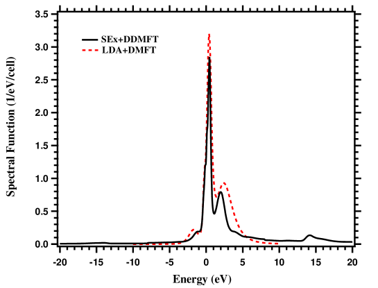
Figure 1: Spectral function of a low-energy (t_2g-only) screened exchange Hamiltonian within standard LDA+DMFT with U=4 eV and J=0.6 eV (red curve) and “Screened Exchange + DDMFT” (“SEx+DDMFT”) (black curve). The calculation uses the same setup as in [49]. Besides the low-energy electronic structure with lower and upper Hubbard bands (at -1.5 eV and 2.0 eV respectively) and a renormalized quasi-particle peak at the Fermi level, the plasmon satellites at $\pm$ 15 eV are clearly visible when the dynamical character of the interaction is included as done in SEx+DDMFT.

To illustrate the effects of the dynamical interactions, we present in Figs. 1 and 4 the spectral function of the t_2g states of the ternary transition metal oxide SrVO₃ within different schemes. SrVO₃ is a perfectly cubic perovskite with d¹ configuration. The crystal field splitting between e_g and t_2g states suggests a many-body description in terms of the t_2g states only, and this was done in the present case. It should be noted however that the contribution of unoccupied e_g states dominates at energies as low as $\sim 2.5$ eV. This issue has been discussed in detail in [21].

The compound is a correlated metal with a moderate quasi-particle renormalisation, and has been the subject of experimental (see e.g. [55, 56, 57, 58, 59] and references thereof) and theoretical (see e.g. [62, 61, 63]) studies over the last 20 years. Detailed spectroscopic, transport, and thermodynamic data are available, and innumerous theoretical works have used this compound as a benchmark compound for new calculational methods [64, 65]. Among others, the first calculations within DDMFT [54] and a dynamical implementation of the combined GW+DMFT scheme [20, 21] have been performed on SrVO₃. An overview with the respective references can be found in [20, 21].

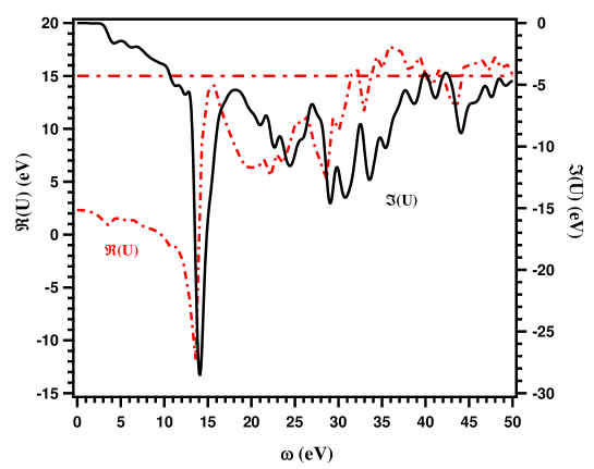
Figure 2: Dynamical interaction for a t_2g-only Hamiltonian for SrVO₃ calculated within the cRPA approximation.

Figure 1 displays a calculation for SrVO₃ within DDMFT with the dynamical interaction calculated from the cRPA. Here, a screened exchange Hamiltonian was used as the one-body part of the Hamiltonian, following the proposal of “Screened Exchange Dynamical Mean Field Theory” of Refs. [49, 48]. Technical details of the calculation can be found in [49]. The t_2g states present at the Fermi level are narrowed into a thin quasi-particle peak, and lower and upper Hubbard bands are visible at -1.5 eV and 2.0 eV respectively. The dynamical interactions lead moreover to an additional transfert of spectral weight from the low-energy part of the spectrum to high energy (plasmon-) satellites, appearing at $\pm$ 15 eV. They correspond to photoemission or inverse photoemission processes that imply the creation or destruction of a bosonic excitation of 15 eV. Their energy is compatible with the plasmon features measured at multiples of 15 eV within low-energy electron diffraction measurements for the related SrTiO₃ [53].

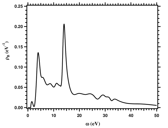
Figure 3: Spectral function $\rho_{B}$ of the bosonic factor $B(\tau)$ for SrVO₃. The strong peak at 15 eV corresponds to the plasmon seen in $\mathcal{U}$. A second “sub-plasmon” is visible around 5 eV. This feature is more clearly seen in the fully screened interaction $W$, since at this energy there is a collective plasmon corresponding to the t_2g charge only. Since transitions within this manifold are cut out when calculating $\mathcal{U}$, only remnants of this feature (surviving due to hybridisation effects) are left within $\mathcal{U}$. Convolution of this curve with the spectral function corresponding to a calculation with static interactions generates the final spectral function. The pronounced peak structures can therefore be directly related to satellite features in the final spectra.

The most interesting aspect in the light of the present discussion is the appearance of the high-energy satellites structures, along with the corresponding spectral weight transfert. Since the overall spectral function is normalised, the appearance of satellites necessarily reduces the spectral weight in the low-energy part of the spectrum. The distribution of spectral weight between the low-energy part (-2 eV to 2eV) around the Fermi level, and the bosonic satellite structures corresponds to the values discussed above: the imaginary part of $\mathcal{U}$ (Figure 2) leads to a $Z_{B}$ factor (Eq. (15)) of 0.6, corresponding to a ratio of 0.6:0.4 for the low-energy spectral weight to the weight of the high-energy satellites.

These spectral properties are thus the direct consequence of the dynamical interaction, plotted in Figure 2. As a partially screened interaction $\mathcal{U}$ is related to a (partial) charge-charge response function, and as such has real and imaginary parts (red and black lines respectively) related by a Kramers-Kronig relation. The real part is characterized by its low-energy value of about 3 eV, corresponding to the usual static Hubbard interaction and its high-energy tail recovering the unscreened interaction in the infinite frequency limit. The change of regime happens at the plasma frequency of about 15 eV. The imaginary part can be understood as the density of screening modes (plasmons, particle-hole excitations …). The sharp peak at 15 eV corresponds to the plasmon that is responsible for the pronounced structure of the real part.

To illustrate more clearly the consequences of the dynamical interaction, we present in Figure 4 a series of calculations where we have a started from a standard LDA+DMFT calculation with static interactions (blue curve) and used this curve as an approximation to the spectral function $A_{stat}$ in Eq. (14). The black curve is obtained by performing the convolution with the bosonic spectral weight function $\rho_{B}$ of Eq. (15), see Figure 3 and the Appendix for details. Besides the case of the physical $\rho_{B}$, we show two cases where the electron-boson coupling has been artificially enhanced. This is done by simply multiplying the spectral distribution of modes $\Im\mathcal{U}$ by multiplicative factors (red and greens curves).

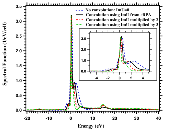
Figure 4: Spectral function of a low-energy (t_2g-only) Hamiltonian produced within a simple model construction: we use an LDA+DMFT spectral function calculated for a static interaction of U=4 eV, J=0.6 eV as approximation to the spectral function $A_{aux}$ in Eq. (14), and obtain the final spectral function by performing the convolution with the bosonic spectral weight function $\rho_{B}$ of Eq. (15). Besides the case of the physical $\rho_{B}$, we show two cases where the electron-boson coupling has been artificially enhanced. This is done by simply multiplying the spectral distribution of modes $\Im\mathcal{U}$ by multiplicative factors.

The figure nicely demonstrates the increasing spectral weight transfert when the electron-boson coupling becomes larger. Now, even the second plasmon satellite structure at 30 eV, corresponding to the creation of two 15 eV plasmons can be seen. Also, smaller satellite features, corresponding to a sub-plasmon at about 5 eV that carry too little spectral weight to clearly appear in the physical case now become visible. The spectral weight transfert to higher energy not only reduces the low-energy spectral weight, but also leads to a corresponding reduction of the energy scales in the low-energy zero plasmon part of the spectrum. This is expected: indeed, the mechanism of reduction is to rescale all hoppings with $Z_{B}$. For a mathematical derivation of this relation, see [54]. Physically it can be understood by noting that the basis that diagonalizes the electron-boson Hamiltonian corresponds to polaronic states, electrons dressed by their respective screening clouds. This “electronic polaron” effect [13, 66, 42] effectively enhances the masses of the charge carriers and translates itself into a narrowed band width.

7 Conclusions and perspectives: What measurable consequences to the physics of dynamical screening?

We close this work with a discussion of measurable consequences of the above phenomena. Obviously, a first indicator for the physics discussed above are satellite structures. Indeed, plasmonic satellites are ubiquitous in photoemission spectroscopy and have – in the past – been considered rather as a nuisance. A systematic investigation, however, could provide extremely useful information about the strength of Coulomb interactions and screening as well as mobile charge carriers. An effect that is harder to observe is the reduction of spectral weight, since photoemission spectroscopy does not have access to absolute values of the spectral function. Probes that assess spectral weight as absolute values, however, such as optical measurements, should be sensitive to this kind of effects. As discussed above, it should also be possible to diagnose the spectral weight reduction as a reduction in hoppings (and therefore bandwidth). This raises however the question of the suitable starting band structure. Indeed, as discussed in [48], there is no a priori reason to use the Kohn-Sham band structure of DFT as input to a many-body calculation. If a generalized one-body Hamiltonian, based on screened exchange, is employed there is a large compensation effect between band widening by screened exchange and the band narrowing by $Z_{B}$. As far as only questions of overall bandwidth are concerned, a many-body calculation with static interaction and using a DFT Hamiltonian is then in fact quite a good approximation. If the spectral weight was assessible quantitatively from experiment, serious discrepancies should however be observed. Finally, we also note that the reshuffling of states around the Fermi level is also expected to impact the magnetic properties of compounds with high densities of states. Ref. [48] for example, explained the absence of ferromagnetism in BaCo₂As₂ by the rearrangement of electronic states around the Fermi level when corrections due to screened exchange and dynamical interactions are included.

The related BaFe₂As₂ compound is an example where satellite features of the above kind have been identified in photoemission spectra (see the data in [67, 68] and the discussion in [51]). Similar satellite features are also ubiquitous in transition metal oxides [71, 69, 70]. Still, systematic studies of such effects have at present not yet been worked out and can be expected to bring additional valuable information concerning the response properties of solids, the strength of electronic correlations and their first principles description.

8 Acknowledgements

This work would not have been possible without the series of recent works on downfolding techniques for many-body interactions, GW+DMFT and dynamical screening [24, 25, 54, 50, 51, 14, 18, 19, 20, 21, 22, 52, 49]. SB thanks her respective coauthors F. Aryasetiawan, T. Ayral, M. Casula, M. Ferrero, A. Georges, P. Hansmann, M. Imada, H. Jiang, I. Krivenko, A. Millis, T. Miyake, O. Parcollet, A. Rubtsov, J.M. Tomczak, L. Vaugier, P. Werner for the enjoyable collaborations and D. D. Sarma, V. Brouet, H. Ding, A. Fujimori, K. Maiti, P. Richard and T. Yoshida for stimulating discussions. Our special thanks go to Ashish Chainani for his interest in this work, his careful reading of the manuscript and most useful suggestions.
The work was further supported by the European Research Council under project 617196 (CORRELMAT) and IDRIS/GENCI under project t2015091393.

9 Appendix

In this Appendix, we comment more precisely on the way we proceed to artificially enhance the plasmonic couplings, in order to plot Figure 4. Indeed, we make a transformation that allows us to recover the Lang-Firsov limit at low-energy and the DALA approximation at high energy. Starting from a spectral function $A$ without plasmonic interactions and a bosonic spectral function $\rho_{B}$ that corresponds to a transfer of weight $1-Z_{B}$ to plasmonic excitations, we first define $\tilde{A}^{aux}(\omega)=A(\omega/Z_{B})/Z_{B}$. This spectral function is still normalized and corresponds to the Lang-Firsov limit, where the effective mass is enhanced by $Z_{B}^{-1}$ without taking into account any spectral weight transfer. We then calculate the final spectral function $\tilde{A}$ in the DALA form:

$$\tilde{A}(\omega)=\int_{-\infty}^{+\infty}d\epsilon\tilde{A}^{aux}(\epsilon)\rho_{B}(\omega-\epsilon)\left[n_{F}(\epsilon)+n_{B}(\epsilon-\omega)\right]$$

where $\rho_{B}$ has a regular part $\rho_{B}^{regular}$ and a delta peak of weight $Z_{B}$:

$$\tilde{A}(\omega)=Z_{B}\tilde{A}^{aux}(\omega)+\int_{-\infty}^{+\infty}d\epsilon\tilde{A}^{aux}(\epsilon)\rho_{B}^{regular}(\omega-\epsilon)\left[n_{F}(\epsilon)+n_{B}(\epsilon-\omega)\right]$$

.

In order to articially enhance the effect of the plasmons, we multiply $\Im\mathcal{U}(\omega)$ by the respective factors. This procedure corresponds to a uniform enhancement of the plasmon-electron coupling for all plasmon frequencies, and translates itself into a highly nonlinear modification of the Boson spectral function $\rho_{B}$ entering the convolution above [50].

References

- [1] Lars Hedin, Phys. Rev., 139(3A):A796–A823, Aug 1965.
- [2] L. Hedin and S. Lundqvist. Solid State Physics, volume 23. Academic, New York, 1969.
- [3] F. Aryasetiawan and O. Gunnarsson, Rep. Prog. Phys. 61, 237 (1998)
- [4] G. Onida et al., Rev. Mod. Phys. 74, 601 (2002).
- [5] A. Georges, G. Kotliar, W. Krauth, and M. J. Rosenberg, Rev. Mod. Phys. 68, 13 (1996)
- [6] Anisimov, V. I., Poteryaev, A. I., Korotin, M. A., Anokhin, A. O. & Kotliar, G. J. Phys.: Cond. Matt. 9, 7359 (1997).
- [7] Lichtenstein A. I. & Katsnelson, M. I. Phys. Rev. B 57, 6884 (1998).
- [8] S. Biermann, Electronic Structure of Transition Metal Compounds: DFT-DMFT Approach, in Encyclopedia of Materials: Science and Technology, pp. 1-9, Eds. K. H. Jürgen Buschow, R. W. Cahn, M. C. Flemings, B. Ilschner (print) and E. J. Kramer, S. Mahajan, P. Veyssière (updates), Elsevier Oxford (2006). DOI: 10.1016/B0-08-043152-6/02104-5, http://www.sciencedirect.com/science/article/B7NKS-4KF1VT9-2HD/2/7e81915568aa0a7f6b47e54f9a97eaf9
- [9] G. Kotliar and D. Vollhardt, Physics Today 57, 3 53 (2004).
- [10] K. Held and I. A. Nekrasov and G. Keller and V. Eyert and N. Blümer and A. K. McMahan and R. T. Scalettar and Th. Pruschke and V. I. Anisimov and D. Vollhardt, Psi-k Newsletter, 56 2003, http://psi-k.dl.ac.uk/newsletters/News56/Highlight56.pdf
- [11] M. Aichhorn, L. Pourovskii, V. Vildosola, M. Ferrero, O. Parcollet, T. Miyake, A. Georges and S. Biermann, Phys. Rev. B 80, 085101 (2009).
- [12] F. Lechermann, A. Georges, A. Poteryaev, S. Biermann, M. Posternak, A. Yamasaki, and O. K. Andersen, Phys. Rev. B 74 125120 (2006)
- [13] S. Biermann, J. Phys.: Condens. Matter 26 173202 (2014),
- [14] S. Biermann, F. Aryasetiawan, and A. Georges. Phys. Rev. Lett., 90:086402, Feb 2003.
- [15] S. Biermann, F. Aryasetiawan, and A. Georges. Proceedings of the NATO Advanced Research Workshop on ”Physics of Spin in Solids: Materials, Methods, and Applications” in Baku, Azerbaijan, Oct. 2003. NATO Science Series II, Kluwer Academic Publishers B.V, 2004.
- [16] F. Aryasetiawan, S. Biermann, and A. Georges. Proceedings of the conference ”Coincidence Studies of Surfaces, Thin Films and Nanostructures”, Ringberg castle, Sept. 2003, 2004.
- [17] P. Sun and G. Kotliar, Phys. Rev. Lett. 92 196402 (2004)
- [18] Thomas Ayral, Philipp Werner, and Silke Biermann. Phys. Rev. Lett., 109:226401, Nov 2012.
- [19] Thomas Ayral, Silke Biermann, and Philipp Werner. Phys. Rev. B, 87:125149, Mar 2013.
- [20] Jan M. Tomczak, Michele Casula, T. Miyake, Ferdi Aryasetiawan, and Silke Biermann. epl, 100:67001, 2012.
- [21] Jan M. Tomczak, Michele Casula, T. Miyake, and Silke Biermann. Phys. Rev. B, submitted. Available electronically as arXiv2013.
- [22] P. Hansmann, T. Ayral, L. Vaugier, P. Werner, and S. Biermann. Phys. Rev. Lett., 110:166401, Apr 2013.
- [23] C.O. Almbladh, U. von Barth, and R. van Leeuwen. Int. J. Mod. Phys. B, 13:535, 1999.
- [24] F. Aryasetiawan, M. Imada, A. Georges, G. Kotliar, S. Biermann, and A. I. Lichtenstein. Phys. Rev. B, 70(19):195104, Nov 2004.
- [25] Loïg Vaugier, Hong Jiang, and Silke Biermann. Phys. Rev. B, 86:165105, Oct 2012.
- [26] Takashi Miyake and F. Aryasetiawan. Phys. Rev. B, 77:085122, Feb 2008.
- [27] F. Aryasetiawan, K. Karlsson, O. Jepsen, and U. Schönberger. Phys. Rev. B, 74:125106, Sep 2006.
- [28] Jan M. Tomczak, T. Miyake, and F. Aryasetiawan. Phys. Rev. B, 81(11):115116, Mar 2010.
- [29] Takashi Miyake, Leonid Pourovskii, Veronica Vildosola, Silke Biermann, and Antoine Georges. J. Phys. Soc. Jap. Suppl. C, 77:99, 2008.
- [30] Kazuma Nakamura, Ryotaro Arita, and Masatoshi Imada. J. Phys. Soc. Jap., 77:093711, 2008.
- [31] Takashi Miyake, Kazuma Nakamura, Ryotaro Arita, and Masatoshi Imada. J. Phys. Soc. Jap., 79:044705, 2010.
- [32] Masatoshi Imada and Takashi Miyake. J. Phys. Soc. Jap., 79:112001, 2008.
- [33] Jan M. Tomczak, L.V. Pourovskii, L. Vaugier, Antoine Georges, and Silke Biermann. Proc. Nat. Ac. Sci. USA, 2013.
- [34] Ersoy Şaşıoğlu, Christoph Friedrich, and Stefan Blügel. Phys. Rev. B, 83(12):121101, Mar 2011.
- [35] Cyril Martins, Markus Aichhorn, Loïg Vaugier, and Silke Biermann. Phys. Rev. Lett., 107:266404, Dec 2011.
- [36] N. Xu et al. Phys. Rev. X 3 011006 (2013)
- [37] J. Ma, A. van Roekeghem, P. Richard, Z. Liu, H. Miao, L. Zeng, N. Xu, M. Shi, C. Cao, J. He, G. Chen, Y. Sun, G. Cao, S. Wang, S. Biermann, T. Qian, H. Ding Phys. Rev. Lett. 113 266407 (2014).
- [38] E. Razzoli, C. E. Matt, M. Kobayashi, X.-P. Wang, V. N. Strocov, A. van Roekeghem, S. Biermann, N. C. Plumb, M. Radovic, T. Schmitt, C. Capan, Z. Fisk, P. Richard, H. Ding, P. Aebi, J. Mesot, M. Shi Physical Review B 91 214502 (2015).
- [39] A. van Roekeghem, P. Richard, X. Shi, S. Wu, L. Zen, B. I. Saparov, Y. Ohtsubo, S. Su, T. Qian, A. Safa-Sefat, S. Biermann and H. Ding, arXiv:1505.00753.
- [40] Philipp Hansmann, Loig Vaugier, Hong Jiang, and Silke Biermann. J. Phys. Cond. Matt., 25:094005, 2013.
- [41] Li Huang and Yilin Wang. Europhys. Lett., 99:67003, 2012.
- [42] Lars Hedin. J. Phys. Condens. Matter 11(42):R489–R528 (1999).
- [43] F. Aryasetiawan, L. Hedin, K. Karlsson. Phys. Rev. Lett. 77 2268 (1996).
- [44] M. Guzzo, G. Lani, F. Sottile, P. Romaniello, M. Gatti, J. J. Kas, J. J. Rehr, M. G. Silly, F. Sirotti, L. Reining Phys. Rev. Lett. 107 166401 (2012).
- [45] M. Gatti and M. Guzzo, Phys. Rev. B 87 155147 (2013).
- [46] J. J. Kas, F. D. Vila, J. J. Rehr, and S. A. Chambers Phys. Rev. B 91, 121112(R) (2015).
- [47] K. Nakamura, Y. Nohara, Y. Yoshimoto, Y. Nomura, arXiv:1511.00218
- [48] Ambroise van Roekeghem, Thomas Ayral, Jan M. Tomczak, Michele Casula, Nan Xu, Hong Ding, Michel Ferrero, Olivier Parcollet, Hong Jiang, Silke Biermann, Phys. Rev. Lett. 113 266403 (2014).
- [49] Ambroise van Roekeghem, Silke Biermann, Europhysics Letters 108 57003 (2014)
- [50] Michele Casula, Alexey Rubtsov, and Silke Biermann. Phys. Rev. B, 85:035115, Jan 2012.
- [51] Philipp Werner, Michele Casula, Takashi Miyake, Ferdi Aryasetiawan, Andrew J. Millis, and Silke Biermann. Nat. Phys., pages 1745–2481, 2012.
- [52] I. Krivenko, S. Biermann, Phys. Rev. B 91 155149 (2015)
- [53] S. Kohiki, M. Asai, H. Yoshikawa, S. Fukushima, M. Oku and Y. Waseda, Phys. Rev. B 62 7964 (2000).
- [54] M. Casula, Ph. Werner, L. Vaugier, F. Aryasetiawan, T. Miyake, A. J. Millis, and S. Biermann. Phys. Rev. Lett., 109:126408, Sep 2012.
- [55] K. Maiti and D. D. Sarma and M. J. Rozenberg and I. H. Inoue and H. Makino and O. Goto and M. Pedio and R. Cimino Europhys. Lett. 55 2 246 (2001).
- [56] Kalobaran Maiti, U. Manju, Sugata Ray, Priya Mahadevan, I. H. Inoue, C. Carbone, and D. D. Sarma. Phys. Rev. B, 73:052508, Feb 2006.
- [57] A. Sekiyama, H. Fujiwara, S. Imada, S. Suga, H. Eisaki, S. I. Uchida, K. Takegahara, H. Harima, Y. Saitoh, I. A. Nekrasov, G. Keller, D. E. Kondakov, A. V. Kozhevnikov, Th. Pruschke, K. Held, D. Vollhardt, and V. I. Anisimov. Phys. Rev. Lett., 93:156402, Oct 2004.
- [58] M. Takizawa, M. Minohara, H. Kumigashira, D. Toyota, M. Oshima, H. Wadati, T. Yoshida, A. Fujimori, M. Lippmaa, M. Kawasaki, H. Koinuma, G. Sordi, and M. Rozenberg. Phys. Rev. B, 80:235104, Dec 2009.
- [59] K. Morikawa, T. Mizokawa, K. Kobayashi, A. Fujimori, H. Eisaki, S. Uchida, F. Iga, and Y. Nishihara. Phys. Rev. B, 52:13711–13714, Nov 1995.
- [60] S. Aizaki, T. Yoshida, K. Yoshimatsu, M. Takizawa, M. Minohara, S. Ideta, A. Fujimori, K. Gupta, P. Mahadevan, K. Horiba, H. Kumigashira, and M. Oshima. Phys. Rev. Lett. 109, 056401 (2012).
- [61] E. Pavarini, S. Biermann, A. Poteryaev, A. I. Lichtenstein, A. Georges, and O. K. Andersen. Phys. Rev. Lett. 92(17):176403, 2004.
- [62] Ishida, H. & Liebsch, A. Phys. Rev. B 81, 054513 (2010).
- [63] R. J. O. Mossanek, M. Abbate, T. Yoshida, A. Fujimori, Y. Yoshida, N. Shirakawa, H. Eisaki, S. Kohno, P. T. Fonseca, and F. C. Vicentin. Phys. Rev. Lett. 79(3):033104, 2009.
- [64] T. Miyake, C. Martins, R. Sakuma, and F. Aryasetiawan. Phys. Rev. B, 87:115110, (2013).
- [65] Yusuke Nomura, Merzuk Kaltak, Kazuma Nakamura, Ciro Taranto, Shiro Sakai, Alessandro Toschi, Ryotaro Arita, Karsten Held, Georg Kresse, and Masatoshi Imada. Phys. Rev. B, 86:085117, Aug 2012.
- [66] A. Macridin, G. A. Sawatzky, M. Jarrell Phys. Rev. B 69, 245111 (2003).
- [67] Ding, H., et al., J. Phys.: Condens. Matter 23, 135701 (2011).
- [68] Yi, M., et al., Phys. Rev. B 80, 024515 (2009).
- [69] R. Eguchi, A. Chainani, M. Taguchi, M. Matsunami, Y. Ishida, K. Horiba, Y. Senba, H. Ohashi, and S. Shin Phys. Rev. B 79, 115122 (2009)
- [70] P.A. Bhobe, A. Chainani, M. Taguchi, R. Eguchi, M. Matsunami, T. Ohtsuki, K. Ishizaka, M. Okawa, M. Oura Y. Senba, H. Ohashi, M. Isobe, Y. Ueda, S. Shin, Phys. Rev. B 83 165132 (2011).
- [71] M. Z. Hasan et al., Phys. Rev. Lett. 92, 246402 (2004).