Spin Physics through QCD Instantons
Abstract
We review some aspects of spin physics where QCD instantons play an important role. In particular, their large contributions in semi-inclusive deep-inelastic scattering and polarized proton on proton scattering. We also review their possible contribution in the -odd pion azimuthal charge correlations in peripheral scattering at collider energies.
I introduction
Dedicated lattice simulations have revealed that the QCD vacuum is characterized by non-trivial topological fluctuations Leinweber et al. (1999, 2004). Instantons and anti-instantons are extrema of the 4-dimensional Euclidean action that carry unit topological charge. They correspond to tunneling between degenerate vaccua. The instanton liquid model with interacting instantons and anti-instantons account for important features of the QCD vacuum, such as the spontaneous breaking of chiral symmmetry and the large mass for the meson Schäfer and Shuryak (1998); Nowak et al. (1996). It does not account for confinement of static charges. Recently, it was noted that twisted instantons and anti-instantons with finite Polyakov lines preserve most of the features of the instanton liquid model and do account for confinement. QCD instantons may contribute substantially to small angle hadron-hadron scattering Shuryak and Zahed (2000); Nowak et al. (2001); Shuryak and Zahed (2004a); Kharzeev and Levin (2000); Dorokhov and Cherednikov (2005) and possibly gluon saturation at HERA Ringwald and Schrempp (2001); Schrempp and Utermann (2003), as evidenced by recent lattice investigations Giordano and Meggiolaro (2010, 2011).
A number of semi-inclusive DIS experiments carried by the CLAS and HERMES collaborations Airapetian et al. (2005, 2009); Avakian et al. (2010), and more recently with polarized protons on protons by the STAR and PHENIX collaborations Abelev et al. (2008); Eyser (2006); Adams et al. (1991), have revealed large spin asymmetries in polarized lepton-hadron and hadron-hadron collisions at collider energies. These effects are triggered by -odd contributions in the scattering amplitude. Perturbative QCD does not support the -odd contributions, which are usually parametrized in the initial state (Sivers effect) Sivers (1990, 1991) or the final state (Collins effect) Collins (1993); Collins et al. (1994). Non-perturbative QCD with instantons allow for large spin asymmetries as discussed by Kochelev and others Kochelev (2000); Dorokhov et al. (2009); Ostrovsky and Shuryak (2005); Qian and Zahed (2012). In Kochelev (2000) a particularly large Pauli form factor was noted, with an important contribution to the Single Spin Asymmetry (SSA) in polarized proton on proton scattering.
In this paper, we review some recent developments regarding our understanding of spin physics in the instanton liquid model. Assuming that the vacuum is populated by semi-classical but interacting instatons and anti-instantons, with the vacuum parameters fixed by the spontaneous breaking of chiral symmetry in bulk, we explicit their effects on semi-inclusive DIS processes as well as singly polarized scattering. In both cases, uncorrelated instantons or anti-instatons are at work. We show that the effects of correlations between instantons and anti-instantons through fluctuations are also important in both doubly polarized scattering as well as through -odd effects in peripheral scattering.
The paper is organized as follows: in section II we detail the role of a single instanton and anti-instanton on the single spin assymetry in semi-inclusive DIS scattering and in polarized scattering. The large instanton contributions appear to be supported by current experiments. In section III we discuss the role of local fluctuations in the compressibility as well as the topological susceptibility in doubly polarized and peripheral scattering. Our conclusions and prospects follow in section IV. In Appendix A we detail the large instanton vertex contribution to both the electromagnetic and chromo-magnetic interactions with the corresponding large magnetic moments.
II Spin effects through one instanton
To best illustrate the important role played by instantons in QCD spin physics, consider a light quark in the fundamental color representation propagating in an external SU(2) colored Yang-Mills gauge field with a chromo-magnetic field and a chromo-electric field field. Generically Shuryak and Zahed (2004b)
| (1) |
with and the SU(2) spin generators. The signs in (1) refer to the chirality of the quark. Large quark amplitudes as polarized zero modes occur when the spin contribution (second term) balances the squared kinetic contribution (first term) in (1). For a self-dual instanton with the negative chirality quark produces a large zero mode state through the magnetic moment term
| (2) |
and similarly for an anti-self-dual anti-instanton. Typically with fm the instanton or anti-instanton size in the vacuum and the strong gauge coupling. So the induced and large magnetic moment in (2) is about where is the density of instantons in the vacuum Schäfer and Shuryak (1998); Nowak et al. (1996). In contrast, perturbative QCD generates small magnetic moments or .
In a similar way, a propagating gluon in an external SU(2) colored SU(2) gauge field acquires also an effective and large magnetic moment. Indeed, the analogue of (1) for a massless gluon in a covariant (Feynman0) background gauge is
| (3) |
The colored gluon in (3) has two physical polarizations as both the longitudinal and time-like are gauge artifacts. Using the decomposition with transverse we have
| (4) |
with playing the role of the spin in the gluon transverse polarization space. (4) is the analogue of (3) with an induced and large magnetic moment as well.
In the Appendix we give a quantitative derivation of these estimates. These semi-classical and large spin effects will now be explored in processes with polarized protons and in peripheral collisions sensitive to -odd fluctuations, in the framework of the instanton liquid model.
II.1 Single Spin Asymmetry Semi-Inclusive Deep Inealstic Scattering
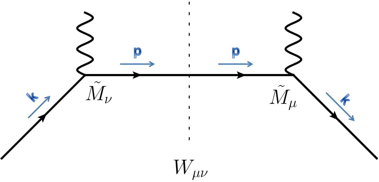
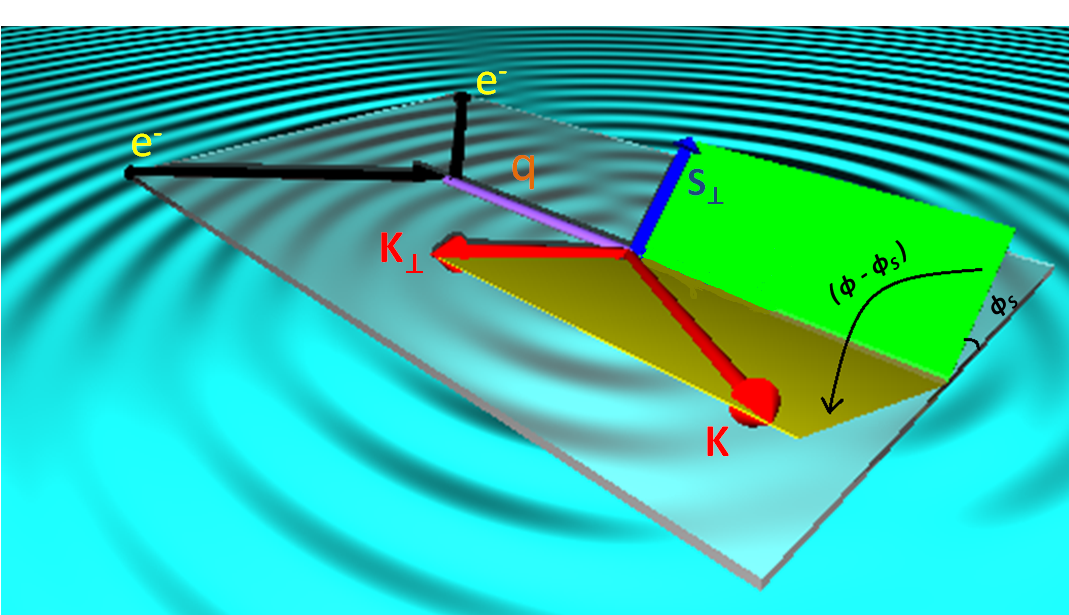
To set up the notations for the semi-inclusive processes in deep inelastic scattering, we consider a proton at rest in the LAB frame with transverse polarization as depicted in Fig. 1. The incoming and outgoing leptons are unpolarized. The polarization of the target proton in relation to the DIS kinematics is shown in Fig. 2. Throughout, the spin dependent asymmetries will be evaluated at the partonic level. Their conversion to the hadronic level will follow the qualitative arguments presented in Kochelev (2000); Dorokhov et al. (2009); Ostrovsky and Shuryak (2005).
In general, the spin averaged leptonic tensor reads
| (5) |
while the color averaged hadronic tensor in the one instanton background reads
| (6) |
with the constituent vertex
| (7) |
that includes both the perturbative and the non-perturbative insertion . In the Appendix we detail its derivation following the original arguments in Moch et al. (1997); Ostrovsky and Shuryak (2005); Qian and Zahed (2012). After color averaging, the result is
| (8) |
with with a modified Bessel function. Here is the instanton size and Schäfer and Shuryak (1998); Nowak et al. (1996) is a typical near-mode in the zero-mode-zone as discussed in the Appendix. The normalized lepton-hadron cross section of Fig.1 follows in the form
| (9) |
with , where is the i-parton electric charge, its momentum fraction distribution and its framentation function.
The perturbative contribution to the hadronic tensor follows from ,
| (10) |
Thus the leading perturbative contribution
| (11) |
with the number of colors. The sum is over the charges of the quarks. The non-perturbative instanton contribution to (9) is a cross contribution in the hadronic tensor in (9) after inserting the one-instanton vertex (8)
where and the short notation is used. If we set and and note that , then (II.1) simplifies
| (13) |
| (14) |
where () is the energy of the incoming (outgoing) (anti)electron. The leading instanton contribution to the total cross section (9) follows by inserting (14) into (10).
| (15) |
where is the spin polarized distribution function for the quark in the transversely polarized proton. The overall sign in (15) is tied with the conventional sign of the proton mass .
To compare with experiment, we will use the spin structure function Airapetian et al. (1998)
| (16) |
Since we are only interested in the SSA in hard scattering processes, we set . A comparison of (18) with (15), yields for the SSA
| (17) |
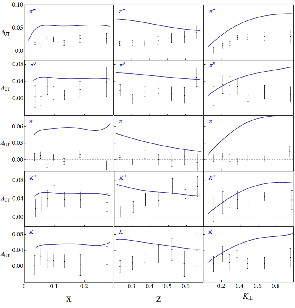
with . This is usually referred to as the Sivers contribution. In Fig. 3 we compare (17) to the results reported by HERMES Airapetian et al. (2009). We use a direct probing of the dependence of the transverse spin asymmetry on . For instance, take the dependent asymmetry of with the empirical parametrizations to fit the reported kinematics from HERMES Airapetian et al. (2009): , , , and . is above 0.97 for all the parametrizations.
II.2 Sinlge Spin Asymmetry in — Transverse parton distribution function
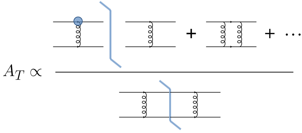
In this section we briefly review the SSA in semi-inclusive and polarized experiments, following the recent analysis in Kochelev and Korchagin (2014); Qian and Zahed (2014). In going through an instanton, the chirality of the light quark can be flipped as we noted in (2). Using the Pauli form factor discussed in the Appendix, the SSA follows from the diagrams of Fig. 5. As noted in Kochelev and Korchagin (2014), the leading diagram contributing to the SSA is displayed in Fig. 5. Note that Fig. 5 is of the same order in as the zeroth order diagram in Fig. 5, since the chirality-flip effective vertex (Eq. 88) is semi-classical and of order . The zeroth order differential cross section reads
| (18) |
The first order differential cross section for the chirality flip reads Potter (1997)
| (19) |
where , is the longitudinal angle of and
| (20) |
From Sec-VII.2 in the Appendix we have
| (21) |
where
| (22) |
To simplify the analysis and compare to the existing semi-inclusive data, we use the kinematics
| (23) |
where is the total energy of the colliding ”partons”. It is simple to show that , which results in SSA. For simplicity, we calculate the first differential cross section with , where the transverse momentum of the outgoing particle lines along the axis. Straightforward algebra yields
where is a hypergeometric function. We note that is much larger than and for . Therefore
| (25) |
The divergence in (25) stems from the exchange of soft gluons in the box diagram. In Kochelev and Korchagin (2014) it was regulated using a constituent gluon mass . For , is parallel to , and this collinear divergence could be regulated by restricting or equivalently setting with an arbitrary constant of order 1. This regularization amounts to the substitution
| (26) |
in Eq. 19, where we have also regulated the collinear divergence when is parallel to . Thus
| (27) |
The regulated SSA is now given by
| (28) |
where the zeroth order cross section in Eq. 18 is used for normalization.
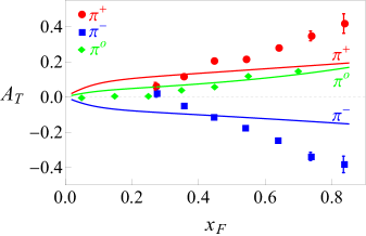
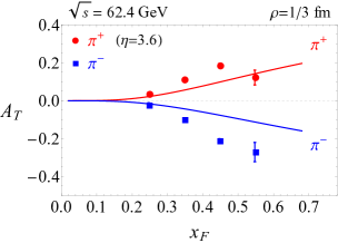
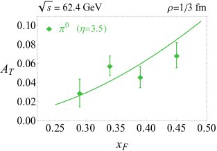
To compare with the semi-inclusive data on , we set and , with and as the spin polarized distribution functions of the valence up-quarks and valence down-quarks in the proton respectively. For forward , and productions, the SSAs are
| (29) |
| (30) |
These results can be compared to the experimental measurements in Skeens (1992). For simplificty, we assume the same fraction for each proton , and is the transverse momentum of the outgoing pion. We then have and . For large , we also have . We set and for the outgoing pions. is the effective instanton density, the typical instanton size and the constitutive quark mass in the instanton vacuum. is the effective gluon mass in the instanton vacuumHutter (1993). In Fig. 6 (left) we display the results (29-31) as a function of the parton fraction for both the charged and uncharged pions at Skeens (1992). Fig. 6 (right) is similar to (left) except for the fact that the divergence in (19) is now regulated by using a constituent gluon mass as in Kochelev and Korchagin (2014). The data in Fig. 7 (left) is from Arsene et al. (2008) and the data (right) is from Adare et al. (2014). In sum, the anomalous Pauli form factor can reproduce the correct magnitude of the observed SSA in polarized for reasonable vacuum parameters.

III Spin Effects through two instantons
III.1 Double Spin Asymmetry in
The same Pauli form factor and vacuum parameters can be used to assess the role of the QCD instantons on doubly polarized and semi-inclusive processes. The Double Spin Asymmetry (DSA) is defined as
| (33) |
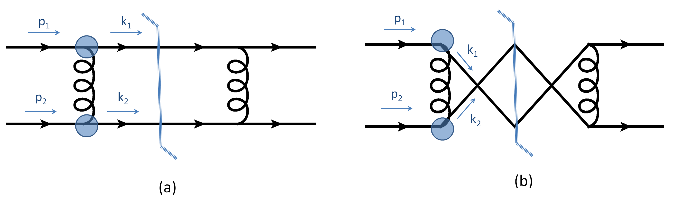
with the proton beam polarized along the transverse direction. The valence quark from the polarized proton exchanges one gluon with the valence quark from the polarized proton as shown in Fig. 8. At large , Fig. 8-(a) is dominant in forward pion production and Fig. 8-(b) is dominant in backward pion production. For Fig. 8-(a), the differential cross section reads
| (34) |
where is propotional to as detailed in VII.2 of the Appendix. To second order, we approximately have
| (35) |
since the instanton liquid is dilute. The contribution to the DSA then follows from simple algebra
| (36) | |||||
after using the identity
| (37) | |||||
with and because the protons are transversely polarized. For an empirical application of (36) we adopt the simple kinematical set up in Eq. IV.1. Thus
| (38) |
After adding the contribution of Fig. 8-(a) and Fig. 8-(b), and averaging over the transverse direction , we finally obtain
| (39) |
Our DSA results can now be compared to future experiments at collider energies. Specifically, our DSA for dijet productions are
| (40) |
| (41) |
| (42) | |||||
To compare our calculations with the experimental results, we use the same kinematics in Fig. 7: and . The value of is from Beringer et al. (2012). Our predictions for charged di-jet production in semi-inclusive DSA are displayed in Fig. 9.

IV -odd effects through Instanton Fluctuations
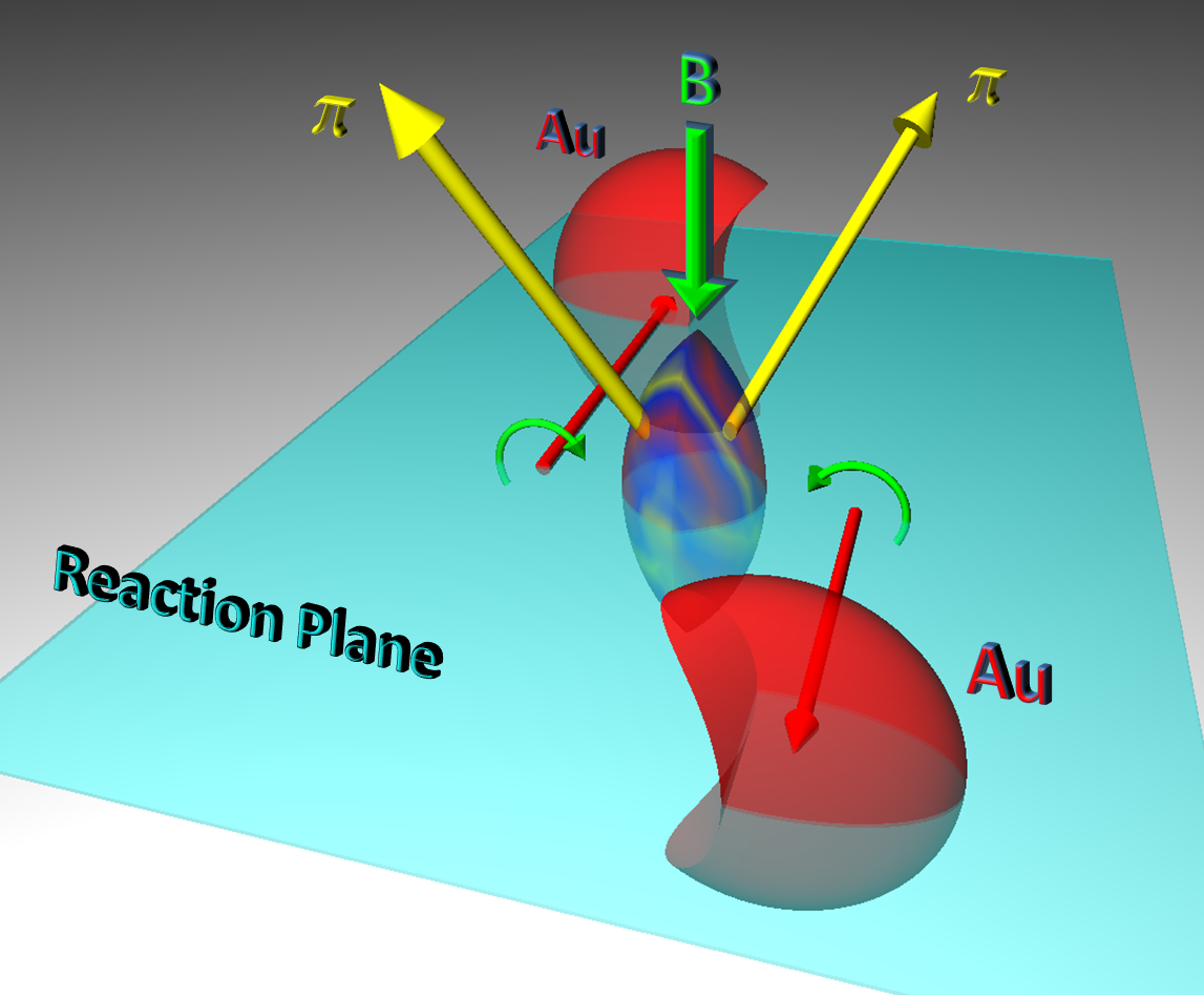
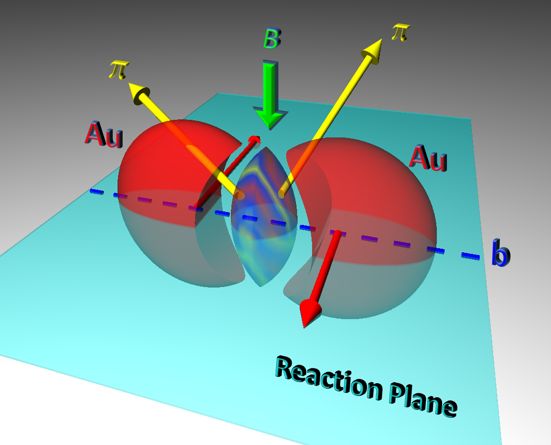
It is commonly accepted that in a typical non-central collision at RHIC as illustrated in Fig. 10 (left), the flying fragments create a large magnetic field that strongly polarizes the wounded or participant nucleons in the final state. The magnetic field is typically at RHIC and at the LHC and argued to last for about 1-3 Skokov et al. (2009). We recall that in these units which is substantial. As a result, large -odd pion azimuthal charge correlations were predicted to take place in peripheral heavy ion collisions Kharzeev et al. (1998); Kharzeev (2006); Kharzeev et al. (2008); Fukushima et al. (2008).
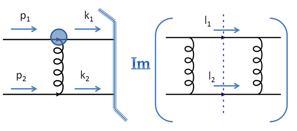
In this section, we would review the analysis in Qian and Zahed (2015) and show that a large contribution to the -odd pion azimuthal charge correlations may stem from the prompt part of the collision as each of the incoming nucleus polarizes strongly the participating nucleons from its partner nucleus during the collision process as illustrated in Fig. 10 (right). The magnetic field is strong but short lived in the initial state, lasting for about for a typical heavy ion collision at current collider energies. Polarized proton on proton scattering can exhibit large chirality flip effects through instanton and anti-instanton fluctuations as we now show.
IV.1 -odd Effects in the Instanton Vacuum
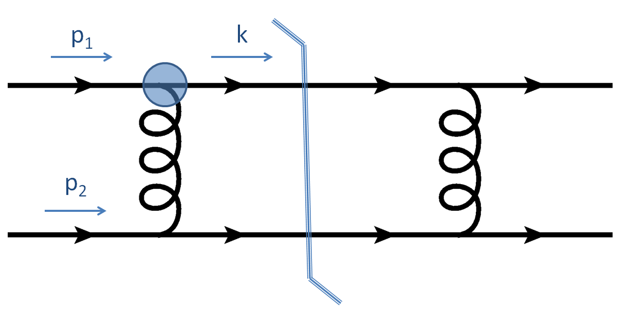
Consider the typical parton-parton scattering amplitude of Fig. 11 with 2-gluon exchanges. In each collision, the colliding “parton” has spin , and thus . The parton from the A-nucleus encounters an instanton or anti-instanton as depicted by the gluonic form-factor. Rewrite the (86)
| (43) |
with stands for an instanton insertion and for an anti-instanton insertion. In establishing (86), the instanton and anti-instanton zero modes are assumed to be undistorted by the prompt external magnetic field. Specifically, the chromo-magnetic field is much stronger than the electro-magnetic field , i.e. or . The deformation of the instanton zero-modes by a strong magnetic field have been discussed in Basar et al. (2012). They will not be considered here.
| (44) |
which can be decomposed into in the dilute instanton liquid. The zeroth order contribution is
| (45) |
where we used . The first order contribution is
| (46) |
after using and . Converting to standard parton kinematics with , and , we obtain for the ratio of the -odd to -even contributions in the differential cross section
| (47) |
Now consider the kinematics appropriate for the collision set up in Fig. 10,
| (48) |
where and are the transverse momentum and total squared energy of the outgoing pion respectively. is the pion longitudinal momentum fraction. Thus
| (49) |
We note that Eq. 49 vanishes after averaging over the instanton liquid background which is -even
| (50) |
since on average .
IV.2 -odd effects in AA Collisions
Now consider hard collisions in peripheral collisions as illustrated inFig. 10 (right). The Magnetic field is strong enough at the collision to partially polarize the colliding protons. Say of the wounded protons from a given nucleus get polarized by the partner colliding nucleus. For simplicity, we set and , with and as the spin polarized distribution functions of the valence up-quarks and valence down-quarks in the proton respectively. We also assume that the outgoing quark turns to and that the outgoing quark turns to . With this in mind, we may rewrite the ratio of differential contributions in (49) following Abelev et al. (2009, 2010); Christakoglou (2011); Selyuzhenkov (2011) as
| (51) |
with or
| (52) |
and
| (53) |
While on average since , in general for the 2-particle correlations. Explicitly
| (54) |
For reasonable values of , as expected Abelev et al. (2009, 2010); Christakoglou (2011); Selyuzhenkov (2011).
A more quantitative comparison to the reported data in Abelev et al. (2009); Selyuzhenkov (2011) can be carried out by estimating the fluctuations of the topological charge in the prompt collision 4-volume . In the latter, 1/2 is the prompt proper time over which the induced magnetic field is active, is the interval in pseudo-rapidity and the transverse collision area for fixed impact parameter . Through simple geometry
| (55) |
where is the radius of two identically colliding nuclei. involves a pair of instanton-antiinstanton. Specifically,
| (56) |
If we denote by the number of instantons and antinstantons in , with their total number, then in the instanton vacuum the pair correlation follows from
| (57) |
Assuming to be large in it follows that Diakonov and Petrov (1984)
| (58) |
The deviation from the Poissonian distribution in the variance of the number average reflects on the QCD trace anomaly in the instanton vacuum or and vanishes in the large limit Diakonov and Petrov (1984). Here is the coefficient of the 1-loop beta function (quenched). Thus
| (59) |
where we have used that the mean in the volume . The topological fluctuations are suppressed by the collision 4-volume. Note that we have ignored the role of the temperature on the the topological fluctuations in peripheral collisions. Temperature will cause these topological fluctuations to deplete and vanish at the chiral transition point following the instanton-anti-instanton pairing Janik et al. (1999). So our results will be considered as upper-bounds.
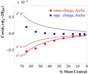
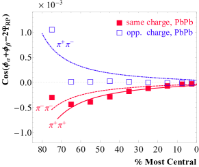
For simplicity, we will set for each parton and . The measured multiplicity spectra in Khandai et al. (2011) at different centralities suggest . We will set in our analysis. We will assume a moderate polarization or in the collision volume for a general discussion. We fix to be the maximum duration of the magnetic field polarization, and set the pseudo-rapidity interval approximately for both STAR Abelev et al. (2009) and ALICE Selyuzhenkov (2011). The radius of the colliding nuclei will be set to where is the atomic number. The centrality is approximated as Aguiar et al. (2004). Our results are displayed in Fig. 12 (left) for and Fig. 12 (middle) for collisions at (STAR), and in Fig. 12 (right) for collisions at (ALICE). We recall that Voloshin (2004)
| (60) |
For the like-charges the results compare favorably with the data. For the unlike charges they overshoot the data especially for the heavier ion. Our results show a difference between and as we only retained the protons in our analysis. The inclusion of the neutrons would result into the same charge correlations for and by isospin symmetry.

V Conclusions and Prospects
Instantons and anti-instantons provide the key building blocks of the instanton liquid model. The latter offers a detailed framework for understanding aspects of the spontaneous breaking of chiral symmetry and the resolution of the U(1) problem. Key to this is the appearance of light quark zero modes of fixed chirality and their de-localization through the formation of an interacting liquid. Some aspects of this model are supported by lattice simulations upon cooling Chu et al. (1993a, b, 1994).
In light of the many phenomenological successes of the instanton liquid model, it is natural to ask about the role of instantons in scattering processes, in particular on spin physics. An essential aspects of the light quark zero modes is the emergence of large constituent masses and (chromo) magnetic moments. Also instantons and anti-instantons correlate strongly the spin with color leading to sizable contributions in spin polarized processes involving light quarks.
This review gives a brief summary of recent advances in the emerging field of spin physics where the induced effects by instantons and anti-instantons in a semi-classical analysis, are sizable in comparison to those usually parametrized using perturbation theory. We stress that the effects we have reported both in polarized electron-proton or proton-proton semi-inclusive scattering, rely solely on the instanton liquid parameters in the vacuum without additional changes. The effects are large and comparable in size with those reported experimentally.
This review also shows that the large spin effects induced by instantons and anti-instantons in polarized experiments may also be present in peripheral collisions where a prompt and large magnetic field can induce a prompt and large polarization although on a short time scale. A simple analysis of the correlated fluctuations between target and projectile protons shows that the effects is of the same magnitude and sign are those reported in the peripheral charged pion azimuthal correlations at collider energies. Again it is important to stress that only the fluctuations expected from instanton vacuum configurations were used.
This review is by no means exhaustive as many new effects can be explored using this framework. One important shortcoming of the instanton liquid model is the lack of confinement as described by an ordering of the eigenvalues of the Polyakov line at low temperature. Some important amendments to the instanton liquid model have been proposed, suggesting that instantons and anti-instantons split into dyons in the confined phase Diakonov and Petrov (2007). It was recently shown that the key chiral effects and U(1) effects in the standard instanton liquid model are about similar to those emerging from the new instanton-dyon liquid model Shuryak and Sulejmanpasic (2012); Shuryak (2014); Larsen and Shuryak (2014); Larsen and Shuryak (2015a, b); Liu et al. (2015a, b). It would be important to revisit the spin effects in this context.
VI acknowledgements
This work was supported in parts by the US-DOE grant DE-FG-88ER40388.
VII Appendix: Effective vertex in instanton background
VII.1 Photon vertex
In this Appendix, we review the derivation of (8) in Qian and Zahed (2012), corresponding to the nonperturbative insertion for photon exchange in the single instanton background. Similar calculations can also be found in Moch et al. (1997); Ostrovsky and Shuryak (2005). According to Brown et al. (1978); Moch et al. (1997); Faccioli and Shuryak (2001); Ostrovsky and Shuryak (2005), the zero mode quark propagator in the single instanton background after Fourier transformation with respect to the incoming momentum is
| (61) |
Note the chirality of the zero mode flips as as depicted in Fig. 13. The incoming quark is left-handed and has momentum (on-shell). is the size of instanton and is the mean virtuality. and are spatial indices, while and are color indices. In Euclidean space, , and Vandoren and van Nieuwenhuizen (2008). The right-handed non-zero mode quark propagator in the single instanton after Fourier transformation with respect to the outgoing momentum is Brown et al. (1978); Moch et al. (1997); Ostrovsky and Shuryak (2005)
| (62) |
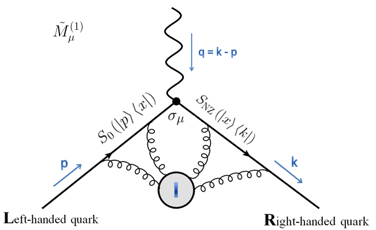
Consider the process depicted in Fig. 13: the incoming left-handed quark meets one instanton and flips its chirality (zero-mode), then exchanges one photon, and finally becomes an outgoing right-handed quark. As a result, the nonperturbative insertion reads
| (63) |
All the other parts of the diagram are trivial in color, therefore we take the trace of color indices and . To further simplify the result, we need the following formula Vandoren and van Nieuwenhuizen (2008)
| (64) |
| (65) |
Combining all the equations above, we obtain
| (66) |
The integration in (66) can be done with the help of the following formula ()
| (67) |
| (68) |
where we used . In our paper Qian and Zahed (2012), we explicitly showed that all terms proportional to vanish. Thus
| (69) |
where As the incoming quark with momentum is on-shell and the mass of the quark is small (), we have
| (70) |
Since in SIDIS, we define . (69) simplifies to
| (71) |
-
•
Left-handed quark () Right-handed quark (zero mode) Right-handed quark ()
where . On the other hand, if we consider
-
•
Right-handed quark () Right-handed quark (zero mode) Left-handed quark ()
instead of (71), we would obtain
| (72) |
where we have taken the conjugate of (71) and replaced . In Qian and Zahed (2012) we used the replacement . We have checked that our final results are left unchanged by this correction. Thus
| (73) |
where denote one or no instanton/anti-instanton. Similarly, for the processes depicted pictorially as
-
•
Right-handed quark () Left-handed quark (zero mode) Left-handed quark ()
-
•
Left-handed quark () Left-handed quark (zero mode) Right-handed quark ()
Thus the result combining both the instanton and anti-instanton contributions
| (74) |
Now, we need to average (74) using the instanton liquid model. The standard averaging in the vacuum is
| (75) |
where by Banks-Casher relation is used . However, we note that in (74) means that we fix an instanton or anti-instanton pertaining to the polarized hadron prior to the averaging. This means that the pertinent eigenvalue distribution instead is
| (76) |
with a typical eigenvalue in the zero-mode-zone. Technically amounts to fixing an instanton or anti-instanton, and averaging over the remainder of the instanton-antiinstanton liquid by removing 1-row and 1-column in the overlap matrix of zero-modes for the fixed instanton or anti-instanton while averaging with in the instanton liquid model. Explictly, this amounts to
| (77) |
Thus
| (78) |
The real part can be re-written as
| (79) | |||||
where . The parts proportional to and vanish as discussed in Kochelev (2003). The imaginary part is
VII.2 Gluon vertex
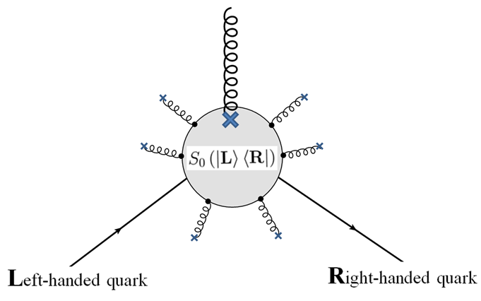
The QCD vacuum is a random ensemble of instantons and anti-instantons interacting via the exchange of perturbative gluons and quasi-zero modes of light quarks and anti-quarks. In the dilute instanton approximation, a typical effective vertex with quarks and gluons attached to an instanton is shown in Fig. 14. The corresponding effective vertex is given by ’t Hooft (1976); Vainshtein et al. (1982); Kochelev (1998),
| (81) |
where is the integration over the instanton orientation in color space and . The incoming and outgoing quarks have small momenta () and is the momentum transferred by the inserted gluon with a form-factor
| (82) |
By expanding (81) to leading order in the inserted gluon field of and integrating over the color indices, we obtain
| (83) |
where is the effective instanton density and is the effective quark mass. In the dilute instanton approximation Shuryak (1982)
| (84) |
where is the average size of the instanton. Hence the induced instanton effective quark-gluon vertex
| (85) |
as illustrated in Fig. 14. In momentum space, the effective vertex is and reads
| (86) |
with and
| (87) |
The averaging of (86) in the instanton liquid gives
| (88) |
where we used
| (89) |
after the analytical continuation to Minkowski Space. (85) yields an anomalously large Quark Chromomagnetic Moment Kochelev (1998)
| (90) |
References
- Leinweber et al. (1999) D. B. Leinweber, J. I. Skullerud, A. G. Williams, and C. Parrinello (UKQCD), Phys. Rev. D60, 094507 (1999), [Erratum: Phys. Rev.D61,079901(2000)], eprint hep-lat/9811027.
- Leinweber et al. (2004) D. B. Leinweber, A. W. Thomas, and R. D. Young, Phys. Rev. Lett. 92, 242002 (2004), eprint hep-lat/0302020.
- Schäfer and Shuryak (1998) T. Schäfer and E. V. Shuryak, Rev.Mod.Phys. 70, 323 (1998), eprint hep-ph/9610451.
- Nowak et al. (1996) M. Nowak, M. Rho, and I. Zahed, Chiral Nuclear Dynamics, v. 1 (World Scientific Publishing Company, Incorporated, 1996), ISBN 9789810210007, URL http://books.google.com/books?id=zhd2QgAACAAJ.
- Shuryak and Zahed (2000) E. V. Shuryak and I. Zahed, Phys. Rev. D62, 085014 (2000), eprint hep-ph/0005152.
- Nowak et al. (2001) M. A. Nowak, E. V. Shuryak, and I. Zahed, Phys. Rev. D64, 034008 (2001), eprint hep-ph/0012232.
- Shuryak and Zahed (2004a) E. V. Shuryak and I. Zahed, Phys. Rev. D69, 014011 (2004a), eprint hep-ph/0307103.
- Kharzeev and Levin (2000) D. Kharzeev and E. Levin, Nucl. Phys. B578, 351 (2000), eprint hep-ph/9912216.
- Dorokhov and Cherednikov (2005) A. Dorokhov and I. Cherednikov, Nucl.Phys.Proc.Suppl. 146, 140 (2005), eprint hep-ph/0412082.
- Ringwald and Schrempp (2001) A. Ringwald and F. Schrempp, Phys. Lett. B503, 331 (2001), eprint hep-ph/0012241.
- Schrempp and Utermann (2003) F. Schrempp and A. Utermann, in 5th Internationa Conference on Strong and Electroweak Matter (SEWM 2002) Heidelberg, Germany, October 2-5, 2002 (2003), eprint hep-ph/0301177.
- Giordano and Meggiolaro (2010) M. Giordano and E. Meggiolaro, Phys.Rev. D81, 074022 (2010), eprint 0910.4505.
- Giordano and Meggiolaro (2011) M. Giordano and E. Meggiolaro, PoS LATTICE2011, 155 (2011), eprint 1110.5188.
- Airapetian et al. (2005) A. Airapetian et al. (HERMES), Phys. Rev. Lett. 94, 012002 (2005), eprint hep-ex/0408013.
- Airapetian et al. (2009) A. Airapetian et al. (HERMES), Phys. Rev. Lett. 103, 152002 (2009), eprint 0906.3918.
- Avakian et al. (2010) H. Avakian et al. (CLAS), Phys. Rev. Lett. 105, 262002 (2010), eprint 1003.4549.
- Abelev et al. (2008) B. Abelev et al. (STAR Collaboration), Phys.Rev.Lett. 101, 222001 (2008), eprint 0801.2990.
- Eyser (2006) K. Eyser (PHENIX Collaboration), AIP Conf.Proc. 842, 404 (2006).
- Adams et al. (1991) D. L. Adams et al. (FNAL-E704), Phys. Lett. B264, 462 (1991).
- Sivers (1990) D. W. Sivers, Phys. Rev. D41, 83 (1990).
- Sivers (1991) D. W. Sivers, Phys. Rev. D43, 261 (1991).
- Collins (1993) J. C. Collins, Nucl. Phys. B396, 161 (1993), eprint hep-ph/9208213.
- Collins et al. (1994) J. C. Collins, S. F. Heppelmann, and G. A. Ladinsky, Nucl. Phys. B420, 565 (1994), eprint hep-ph/9305309.
- Kochelev (2000) N. Kochelev, JETP Lett. 72, 481 (2000), eprint hep-ph/9905497.
- Dorokhov et al. (2009) A. E. Dorokhov, N. I. Kochelev, and W. D. Nowak, Phys. Part. Nucl. Lett. 6, 440 (2009), eprint 0902.3165.
- Ostrovsky and Shuryak (2005) D. Ostrovsky and E. Shuryak, Phys.Rev. D71, 014037 (2005), eprint hep-ph/0409253.
- Qian and Zahed (2012) Y. Qian and I. Zahed, Phys.Rev. D86, 014033 (2012), eprint 1112.4552.
- Shuryak and Zahed (2004b) E. V. Shuryak and I. Zahed, Phys. Rev. D70, 054507 (2004b), eprint hep-ph/0403127.
- Moch et al. (1997) S. Moch, A. Ringwald, and F. Schrempp, Nucl.Phys. B507, 134 (1997), eprint hep-ph/9609445.
- Airapetian et al. (1998) A. Airapetian et al. (HERMES), Phys. Lett. B442, 484 (1998), eprint hep-ex/9807015.
- Kochelev and Korchagin (2014) N. Kochelev and N. Korchagin, Phys.Lett. B729, 117 (2014), eprint 1308.4857.
- Qian and Zahed (2014) Y. Qian and I. Zahed, Phys. Rev. D90, 114012 (2014), eprint 1404.6270.
- Potter (1997) B. Potter (1997).
- Hirai et al. (2006) M. Hirai, S. Kumano, and N. Saito, Phys.Rev. D74, 014015 (2006), eprint hep-ph/0603213.
- Adams et al. (1998) D. Adams et al. (Fermilab E704 Collaboration), Nucl.Phys. B510, 3 (1998).
- Skeens (1992) J. Skeens (E704 Collaboration), AIP Conf.Proc. 243, 1008 (1992).
- Hutter (1993) M. Hutter (1993), eprint hep-ph/9501335.
- Arsene et al. (2008) I. Arsene et al. (BRAHMS), Phys. Rev. Lett. 101, 042001 (2008), eprint 0801.1078.
- Adare et al. (2014) A. Adare et al. (PHENIX), Phys. Rev. D90, 012006 (2014), eprint 1312.1995.
- Beringer et al. (2012) J. Beringer et al. (Particle Data Group), Phys. Rev. D86, 010001 (2012).
- Skokov et al. (2009) V. Skokov, A. Y. Illarionov, and V. Toneev, Int.J.Mod.Phys. A24, 5925 (2009), eprint 0907.1396.
- Kharzeev et al. (1998) D. Kharzeev, R. Pisarski, and M. H. Tytgat, Phys.Rev.Lett. 81, 512 (1998), eprint hep-ph/9804221.
- Kharzeev (2006) D. Kharzeev, Phys.Lett. B633, 260 (2006), eprint hep-ph/0406125.
- Kharzeev et al. (2008) D. E. Kharzeev, L. D. McLerran, and H. J. Warringa, Nucl.Phys. A803, 227 (2008), eprint 0711.0950.
- Fukushima et al. (2008) K. Fukushima, D. E. Kharzeev, and H. J. Warringa, Phys.Rev. D78, 074033 (2008), eprint 0808.3382.
- Qian and Zahed (2015) Y. Qian and I. Zahed, Nucl. Phys. A940, 227 (2015), eprint 1205.2366.
- Basar et al. (2012) G. Basar, G. V. Dunne, and D. E. Kharzeev, Phys.Rev. D85, 045026 (2012), eprint 1112.0532.
- Abelev et al. (2009) B. Abelev et al. (STAR Collaboration), Phys.Rev.Lett. 103, 251601 (2009), eprint 0909.1739.
- Abelev et al. (2010) B. Abelev et al. (STAR Collaboration), Phys.Rev. C81, 054908 (2010), eprint 0909.1717.
- Christakoglou (2011) P. Christakoglou, J.Phys. G38, 124165 (2011), eprint 1106.2826.
- Selyuzhenkov (2011) I. Selyuzhenkov (ALICE Collaboration), PoS WPCF2011, 044 (2011), eprint 1203.5230.
- Diakonov and Petrov (1984) D. Diakonov and V. Y. Petrov, Nucl.Phys. B245, 259 (1984).
- Janik et al. (1999) R. A. Janik, M. A. Nowak, G. Papp, and I. Zahed, AIP Conf.Proc. 494, 408 (1999), eprint hep-lat/9911024.
- Khandai et al. (2011) P. K. Khandai, P. Shukla, and V. Singh, Phys. Rev. C84, 054904 (2011), eprint 1110.3929.
- Aguiar et al. (2004) C. Aguiar, T. Kodama, R. Andrade, F. Grassi, Y. Hama, et al., Braz.J.Phys. 34, 319 (2004).
- Voloshin (2004) S. A. Voloshin, Phys.Rev. C70, 057901 (2004), eprint hep-ph/0406311.
- Chu et al. (1993a) M. C. Chu, J. M. Grandy, S. Huang, and J. W. Negele, Phys. Rev. Lett. 70, 255 (1993a), eprint hep-lat/9211019.
- Chu et al. (1993b) M. C. Chu, J. M. Grandy, S. Huang, and J. W. Negele, Phys. Rev. D48, 3340 (1993b), eprint hep-lat/9306002.
- Chu et al. (1994) M. C. Chu, J. M. Grandy, S. Huang, and J. W. Negele, Phys. Rev. D49, 6039 (1994), eprint hep-lat/9312071.
- Diakonov and Petrov (2007) D. Diakonov and V. Petrov, Phys. Rev. D76, 056001 (2007), eprint 0704.3181.
- Shuryak and Sulejmanpasic (2012) E. Shuryak and T. Sulejmanpasic, Phys. Rev. D86, 036001 (2012), eprint 1201.5624.
- Shuryak (2014) E. Shuryak, Nucl. Phys. A928, 138 (2014), eprint 1401.2032.
- Larsen and Shuryak (2014) R. Larsen and E. Shuryak (2014), eprint 1408.6563.
- Larsen and Shuryak (2015a) R. Larsen and E. Shuryak, Phys. Rev. D92, 094022 (2015a), eprint 1504.03341.
- Larsen and Shuryak (2015b) R. Larsen and E. Shuryak (2015b), eprint 1511.02237.
- Liu et al. (2015a) Y. Liu, E. Shuryak, and I. Zahed, Phys. Rev. D92, 085006 (2015a), eprint 1503.03058.
- Liu et al. (2015b) Y. Liu, E. Shuryak, and I. Zahed, Phys. Rev. D92, 085007 (2015b), eprint 1503.09148.
- Brown et al. (1978) L. S. Brown, R. D. Carlitz, D. B. Creamer, and C.-k. Lee, Phys.Rev. D17, 1583 (1978).
- Faccioli and Shuryak (2001) P. Faccioli and E. V. Shuryak, Phys.Rev. D64, 114020 (2001), eprint hep-ph/0106019.
- Vandoren and van Nieuwenhuizen (2008) S. Vandoren and P. van Nieuwenhuizen (2008), eprint 0802.1862.
- Kochelev (2003) N. Kochelev, Phys.Lett. B565, 131 (2003), eprint hep-ph/0304171.
- ’t Hooft (1976) G. ’t Hooft, Phys.Rev. D14, 3432 (1976).
- Vainshtein et al. (1982) A. Vainshtein, V. I. Zakharov, V. Novikov, and M. A. Shifman, Sov.Phys.Usp. 25, 195 (1982).
- Kochelev (1998) N. Kochelev, Phys.Lett. B426, 149 (1998), eprint hep-ph/9610551.
- Shuryak (1982) E. V. Shuryak, Nucl.Phys. B198, 83 (1982).