Waves in vertically inhomogeneous dissipative atmosphere

Abstract

A method of construction of solution for acoustic-gravity waves (AGW) above a wave source, taking dissipation throughout the atmosphere into account (Dissipative Solution above Source, DSAS), is proposed. The method is to combine three solutions for three parts of the atmosphere: an analytical solution for the upper isothermal part and numerical solutions for the real non-isothermal dissipative atmosphere in the middle part and for the real non-isothermal small dissipation atmosphere in the lower one. In this paper the method has been carried out for the atmosphere with thermal conductivity but without viscosity. The heights of strong dissipation and the total absorption index in the regions of weak and average dissipation are found. For internal gravity waves the results of test calculations for an isothermal atmosphere and calculations for a real non-isothermal atmosphere are shown in graphical form. An algorithm and appropriate code to calculate DSAS, taking dissipation due to finite thermal conductivity into account throughout the atmosphere, are developed. The results of test DSAS calculations for an everywhere isothermal atmosphere are given. The calculation results for DSAS for the real non-isothermal atmosphere are also presented. A method for constructing of the 2x2 Green’s matrix fully taking dissipation into account and allowing to find disturbance from some source of AGW in the atmosphere is proposed.

1 Introduction

The study of acoustic-gravity waves (AGW) in the atmosphere has a long history. The basic properties of AGW propagation were summarized even in Gossard and Hooke (1975). However, dissipationless approach limits the applicability of the results. They apply only to the waves in the lower and middle atmosphere, where weakness of dissipation allows to neglect it. High enough in the upper rarefied atmosphere dissipation becomes the determining factor in the behavior AGW. Therefore, to describe the penetration of AGW in the upper atmosphere it is necessary to involve more complex formalism of the dissipative hydrodynamics. In the dissipative hydrodynamics an analytical description of AGW is obtained in the frames of the isothermal approximation (Lyons and Yanowitch, 1974; Yanowitch, 1967a, b; Rudenko, 1994a, b). However, isothermal approximation models the real atmosphere properties adequately in its upper layers only. Without the isothermal approximation the wave dissipation was taken into account in Vadas (2005). These researches were performed with use of the WKB approximation, which has its limitations. It enables to take into account the weak dissipation in the lower and middle layers of the atmosphere and does not allow to adequately describe the strong effect of dissipation on the wave in the upper atmospheric layers.

This paper is devoted to an AGW solution fully taking dissipation into account. The solution is constructed as an integrated whole for two fundamentally different physical conditions of the atmosphere, with virtually no dissipation in the lower and middle atmosphere and with substantial dissipation, increasing with the height, in the upper atmosphere. The solution has two parameters: real wave frequency and horizontal wave number.

The absence of the flow of energy towards the Earth in the upper layers of the atmosphere is the only boundary condition for the solution; because of dissipativity of the atmosphere, it coincides with the condition of upward attenuation of the solution (from the Earth). The solution exists at all heights. Formally, it can be taken as a solution of the wave problem with some source on the Earth surface. However, wider physical meaning of this solution is that the part of this solution, with real wave frequency and horizontal wave number, in the region above any source located in the atmosphere (or on the Earth’s surface), describes the vertical structure of the disturbance produced by this source there in this region . Region above a source is a part of the atmosphere, the heights of which exceed the upper limit of the source localization; there are no limits for horizontal coordinates of this region. Formally, the solution extends indefinitely in the upper atmosphere. Starting from some height it decreases against the rarefying atmosphere background due to increase of the effect of dissipation with altitude. Given dissipative character of the solution and its aforementioned physical meaning we call it dissipative solution above source (DSAS).

DSAS is necessary final element for the solution of the problem of the wave propagation from a source located in the atmosphere.

Now there are well-developed methods for description of wave phenomena in the real atmosphere, based on the direct numerical solution of hydrodynamic equations, which include a variety of model sources of climate and anthropogenic character: (Hickey et. al., 1997, 1998; Walterscheid and Schubert, 1990; Walterscheid at. al., 2001; Snively and Pasko, 2003, 2005; Snively et. al, 2007; Yu and Hickey, 2007a, b, c; Yu at. al., 2009; Kshevetskii and Gavrilov, 2005; Gavrilov, and Kshevetskii, 2014). These methods are based on direct numerical integration of the nonlinear system of partial differential equations in two- or three-dimensional approximations for stratified atmosphere with viscosity and thermal conductivity and wind stratification. However, these methods are inefficient when describing the perturbation at large distance from the localization of the source, because of their resource consumption and rapid accumulation of numerical errors in the need to increase the grid to ensure sufficient spatial resolution. It is well known that the wave disturbances, propagating far from their sources, are important elements of the dynamics of the atmosphere. Due to increase of their relative amplitudes in height, they manifest themselves in the thermosphere as the main cause of the diverse ionospheric disturbances. The transfer of wave energy and momentum over large distances is provided due to presence of the conditions of waveguide propagation in the temperature inhomogeneities in the lower and middle atmosphere Pierce and Posey (1970). The most effective method to describe the remote signals is to present them as superpositions of the waveguide modes generated by the source (the method of the normal modes). An algorithm, for solving the disturbance propagation problem, based on the method of normal modes, described in detail in Pierce at. al. (1971), where a result of comparison of the calculated and the observed pressure disturbances on the Earth’s surface in the far zone of a nuclear explosion was first presented. In principle, based on the algorithm of Pierce at. al. (1971), synthesizing propagating normal modes, one can calculate the disturbance parameters at any height where the dissipation-free approach, in which Pierce at. al. (1971), built its own algorithm, still holds.

Our main goal is to study the possibility of similar description of the long-range propagation of disturbances in the ionospheric heights. In the ionosphere, according to the basic concept Hines (1960), the so-called travelling ionospheric disturbances (TIDs) are the result of infiltration of the neutral atmosphere disturbances from the lower IGW (internal gravity wave) waveguide channels. In the upper atmosphere in the tropospheric heights the dissipative effect on the wave processes becomes dominant that makes it impossible to ignore and even to take into account approximately the dissipative terms of the wave equations system. As a result, we have to deal with a significantly more complicate problem compared to that of Pierce at. al. (1971).

As in the dissipation-free case, Pierce at. al. (1971), the key element of the disturbance propagation problem is to find the Green’s function (or matrix), for the construction of which we need two solutions: the lower one (below the source) and the upper one (above the source) satisfying the lower and upper boundary conditions, respectively. In the case, when a source is in the range of altitudes where the dissipation-free approximation is applicable, then finding a solution under source can now be considered as a routine problem. Thus, in this case, the key problem is to find a solution above the source for a realistic model of the atmosphere with a full account of dissipation. It is the problem the present paper focuses on. Our approach to this problem bases on matching a solution of the weakly-dissipative wave problem of second order for the lower part of the atmosphere with a solution of the dissipative wave problem of order, higher than second, for the upper part of the atmosphere. It is different essentially, on the level of severity, from the method proposed in its time in Francis (1973a). In the paper Francis (1973a), a solution over the source was obtained with the so-called multi-layer technique, in which the medium in each horizontal layer is considered isothermal with constant coefficients of viscosity and thermal conductivity; so representation of the solution in each such layer is possible in analytical form. When taking dissipation into account, there are, generally speaking, three wave types with three complex values of the square of the vertical wave number, corresponding to (in the weak dissipation case) conventional acoustic-gravity wave (AGW) and two types of purely dissipative oscillations caused by viscosity and thermal conductivity. Francis (1973a) represented the solution in each layer only with AGV solutions, and only two conditions of six ones used for matching solutions of adjacent layers. Such an approach is quite justified in the temperate heights, where dissipation is weak, but obviously incorrect in the strong dissipation regions. Thus, in order to solve the problem, Francis artificially lowered the order of the system of equations from the 6th order up to the second order everywhere. Thus, the structure of wave disturbances in the lower part of the atmosphere and the dispersion characteristics of the modes, captured by the inhomogeneities of the lower atmosphere, the method of Francis allows to calculate sufficiently well, but it obviously is not able to give a correct description of disturbances in the upper atmosphere. The results of Francis are widely used in the theoretical researches and in the interpretation of observations of various disturbances, including those in the upper atmosphere (Shibata and Okuzawa, 1983; Afraimovich at. al., 2001; Vadas and Liu, 2009; Vadas and Nicolls, 2012; Idrus et. al., 2013; Heale at. al., 2014; Hedlin at. al., 2014). Unlike Francis, we use a method of reducing the order of the system of the wave equations up to the second one (in our own version) only for the small-dissipation altitudes where it is justified. Therefore, our method, unlike the method of Francis, gives the possibility to describe disturbances of the upper atmosphere adequately. Another approach to obtain the solution above source is developed in the papers (Lindzen, 1970, 1971; Lindzen and Blake, 1971). This approach, based on the numerical method of the tridiagonal matrix algorithm for the full system of linear dissipative hydrodynamic equations, can be considered quite strict. The only restriction is the circumstance that the hydrostatic approximation is used, which is valid only for sufficiently long-period oscillations (with frequencies much lower than the Brunt-Väisälä frequency). The results obtained on the basis of this approach played an important role in the description of tidal modes and continue to be relevant until now (Forbes and Garrett, 1979; Fesen, 1995; Gavrilov, 1995; Grigor’ev, 1999; Akmaev, 2001; Angelatsi and Forbes, 2002; Yu at. al., 2009).

Thus, our approach to obtaining the solution above source differs from Francis (1973a) by correct consideration of dissipation; as for the papers on the base of Lindzen (1970), it is of more universal character since does not have restrictions caused by usage of the hydrostatic approximation. It should be noted that the dissipation is taken into account in our present paper less complete than in the aforementioned papers. This is due to the fact that we believe it possible, as a first step, consider the viscous dissipation as negligible, taking only the dissipation due to the heat conductivity into account. We use such an approach in connection with the possibility of a simple analytic representation of solutions in heat-conducting thermosphere, which allows us to put the upper boundary conditions more strict at the infinity. Such conditions are more accurate compared with the boundary conditions at some height used in Lindzen (1970). It is also a useful approach as giving a clear understanding of dissipation influence on the wave motion in the upper atmosphere.

Because in reality the dissipation, associated with the thermal conductivity, begins its influence at lower altitude then the viscous dissipation does, our model of the atmosphere can give the real picture of the disturbances in the upper atmosphere sufficiently well, at least, to a certain height. As will be discussed below, taking into account the atmosphere viscosity is, in principle, possible in our approach to finding DSAS. It is also feasibly to include, in the model, the atmosphere wind, which is not considered in this paper.

DSAS formally exists for the entire atmosphere up to the Earth and corresponds in this form (for all heights) to the particular case of a source on the Earth’s surface.If such a solution for certain values of the frequency and horizontal wave number $k_{x}$ satisfies the lower boundary condition, it can be regarded as a solution for a trapped mode.

In general case with the wind, the continuation of DSAS up to the Earth is possible in such cases when the horizontal phase velocity of the wave is large enough so it is not equal to the wind speed at any height. Otherwise, because of the so-called wave destruction (the phenomenon, responsible for the turbulent properties of the real atmosphere), Lindzen (1981), DSAS will be applied only to a certain height and can be used for cases of sources at sufficiently high altitudes. However, the horizontal phase velocities of the waveguide modes, which are responsible for the distant propagation (Francis, 1973b), are of the order of the speed of sound, so the condition of equality of the phase velocity to the wind speed never is satisfied.

It should also be noted that the feature of our method is absence of the need to include in the equations the additional dissipative terms taking into consideration the impact of turbulence in a model manner, without which none of the previously developed methods can work, because of the inherent numerical instability.

DSAS with a full view of the dissipation is most important for the synthesis of the waveforms at fairly high altitudes, where it is impossible to consider dissipation with any approximate method. Such altitudes are typical for TIDs. To synthesize waveforms at lower altitudes the algorithms for non-dissipative atmosphere are sufficient, for example, the above algorithm of Pierce at. al. (1971). Note that the wave forms of the disturbances in the upper atmosphere should be less complicated than those in the middle and lower altitudes, due to the dissipative suppression of multiple waveguide modes of high-frequency sound range. As shown by Francis (1973b), only one or two major IGW modes can take place at ionospheric heights, due to the waveguide leakage and the weak horizontal attenuation.

Our consideration, as well as the general problem of the synthesis of waveforms by normal modes, requires linearity of disturbance at all altitudes. Taking dissipation into account provides drop with height of the disturbance amplitude, relative to the background parameters, in the upper atmosphere from a certain level. This circumstance enables the selection of source amplitude small enough for the disturbance to be linear throughout. At first glance, it may seem that limitations of the source amplitude, to ensure linearity of the disturbance, have to be very strong and so the real sources unlikely satisfy them - since the dissipative suppression of growth of the relative amplitude of the disturbance with height, as a rule, begins at the altitudes, at which the disturbance amplitude can grow by orders of magnitude compared to the amplitude near the Earth. Indeed, the disturbances have likely to be non-linear just above the typical sources localized in space and time. However, we must take into account the fact that only a small part of the disturbance energy is captured by the low-atmosphere waveguides, capable of transferring the wave energy over long distances. In addition, if the main source spectral power is distributed in the high-frequency range (this is typical, for example, for explosions), then the amplitudes of the low-frequency spectrum range, generating waveguide modes, will be significantly less than the main amplitudes of the source. All these factors quite can lead to linearity of the waveguide modes.

Note, in particular, the fact that TIDs are typically very close to harmonical waves (Gossard and Hooke, 1975) says also in favor of the assumption of linearity of the actual responses in the upper atmosphere. Thus, we can assume that the linear solution above the source can be the basis for solving the propagation problem for disturbances in a stratified atmosphere, if the amplitude of the source is small enough, or the ducting propagation only is of interest.

The solution to this problem for a stratified atmosphere within the dissipationless approximation is well known Gossard and Hooke (1975). In this case, we have the second-order problem, i.e. it is formulated as a second-order differential equation or a set of two first-order differential equations equivalent to it. To solve the dissipationless problem with a source the Green’s matrix composed of two second-order problem solutions is used. One of these solutions must satisfy the upper boundary condition and the other must satisfy the condition on the Earth. It is shown in this paper that one can also limit to a second-order problem in the small dissipation approximation for disturbance of not too small vertical scale. Therefore, the solution of the problem with a source is also obtained in this case by means of the second-order Green’s matrix. But the small dissipation approximation is applicable only in the lower and middle parts of the atmosphere. It is not sufficient in the upper part because of increase with altitude of the dissipation effect. So we have to solve a problem of order higher, then second, there.

But even fully taking dissipation into account, one can retain a formalism of a second-order problem to a significant extent if the source is located in the altitude range where dissipation is small. For this it is enough to replace the solution of the second-order problem in the $2\times 2$ Green’s matrix that satisfies the upper boundary condition with DSAS. The Green’s matrix obtained in such a way we will call the extended Green’s matrix. Note that in the atmosphere mainly occur sources for which the method of the extended Green matrix is applicable. These are sources located in the lower and middle atmosphere: EXPLOSIONS tsunami meteorites anthropogenic sources, meteorological phenomena.

Description of an extended tail formally indefinitely outgoing to the upper atmosphere is the main feature of DSAS. However, if a wave is attenuated too much for its extension to the upper atmosphere, the amplitude of the upper atmospheric tail can be so small that the disturbance with such an amplitude is of no interest. On the other hand, if a wave weakly damps when propagating to the upper atmosphere, the relative amplitude of the tail (the ratio of the amplitude to the background) can be too large in the upper atmosphere for the disturbance to be under the linear approximation. In this connection, we investigated effect of dissipation on the AGV propagation. Some characteristics of the wave dissipative loss are introduced and, then, their values are calculated.

We organize our paper as follows. Equations used further to construct a DSAS are derived in Section 2. We have demonstrated the possibility of obtaining from the hydrodynamic equations both a system of four first-order ODEs taking into account thermal conductivity only and, in more general case, a system of six first-order ODEs assuming, besides consideration of thermal conductivity, atmospheric viscosity. Numerical solutions of such systems can be obtained by the standard Runge-Kutta method, if the initial values of the unknowns are given at the specified height. The possibility of including wind stratification in the model of the atmosphere is indicated. To describe waves in the weakly dissipative (lower) part of the atmosphere we obtained a system of two first-order ODE.

Section 3 gives details on the method for an analytical solution for the upper atmosphere with an isothermal temperature distribution. The theory is based on the possibility of describing wave disturbances in an isothermal atmosphere by one sixth-order differential equation in the general case of simultaneous consideration of viscosity and thermal conductivity or fourth-order equation if we consider the thermal-conductivity model of the atmosphere without viscosity. In this paper, we have constructed DSAS for the case of the thermal-conductivity model of the atmosphere without viscosity. In this case, a fourth-order equation reduces to the generalized hypergeometric differential equation (Lyons and Yanowitch, 1974; Yanowitch, 1967a, b; Rudenko, 1994a, b) analytical solutions of which are subsequently used for the isothermal part of the atmosphere. In section 3, we also study the effect of dissipation on the AGV propagation. First, the parameter $z_{c}$, characterizing the heights of the transition to the regime of strong dissipation, is calculated. This parameter is singled out when deriving the hypergeometric differential equation (Lyons and Yanowitch, 1974; Yanowitch, 1967a, b; Rudenko, 1994a, b). In the heights below $z_{c}$, we have approximately classical oscillations corresponding to usual wave types of oscillations without dissipation. In the range of heights higher $z_{c}$, dissipation completely changes nature of oscillations transforming them into purely dissipative waves. It follows from the equations that $z_{c}$ depends only on the wave period for any vertical profile of the atmospheric density, so we calculated it as a function of period. The parameter $z_{c}$, calculated for the isothermal atmosphere, can be used for estimating of the height of the strong dissipation region, depending on wave period, in the real atmosphere. Second, as a dissipation characteristic at the heights below $z_{c}$, we introduced an index of total vertical dissipation . We calculated it both on the basis of the WKB-approximation solution for the non-isothermal thermal-conductive atmosphere and and the analytical solution for isothermal thermal-conductive atmosphere.

Section 4 gives our method for constructing of DSAS. We have carried out this method in the frames of the thermal-conductivity model of the atmosphere without viscosity. In this case, the complete set of wave equations is presented by four first-order ordinary differential equations which, as we show, can be numerically solved in the upper part of the atmosphere, where dissipation is strong, to some height in the middle atmosphere, where dissipation effect is sufficiently small. There are calculation difficulties not allowing us to use a complete set of wave equations in the lower part of the atmosphere. On the other hand, dissipation is small there. This allowed us to reduce the fourth-order problem in the lower part of the atmosphere to a second-order problem. Thus, DSAS is constructed of the solutions for three height ranges in the direction from the upper part of the atmosphere to the Earth: an analytical solution for the isothermal upper atmosphere (I); a numerical solution of the system of four ODEs in a non-isothermal upper atmosphere until the height of $z_{t}$ on which the dimensionless kinematic thermal conductivity reaches a sufficient smallness (II); a solution of the system of two ODEs for the small dissipation approximation in the region below $z_{t}$ up to the Earth’s surface (III). We will further also call the height ranges I, II, III lower middle and upper parts of the atmosphere, respectively.

An analytical solution (I), satisfying the condition of upward attenuation, is a superposition of a superposition of some two solutions, having asymptotics each of which attenuates upward; the coefficients of these solutions are arbitrary. DSAS is continuous at the boundary of the regions (I) and (II) because an analytical solution (I) at this boundary gives four initial values for solving the system of four ODEs numerically in the region (II).

As for the boundary of the regions (II) and (III) then we applied our method for matching the solutions (II) and (III) there. Matching solutions (II) and (III) is important element in constructing DSAS. It is clear that the solutions corresponding to different approximations can not be match arbitrarily closely at the boundary. However, it is also clear that this is not required, the smallness of jumps is enough. Therefore matching the solutions (II) and (III) carries out as follows. We take values of any two components from four components of the solution (II) at the boundary of the regions (II) and (III) (the height $z_{t}$) as initial values for solving the system of two ODEs numerically in the region (II). For two other components, we provide sufficient smallness of the jump at the height $z_{t}$,using the condition of minimization of the jumps to find the ratio between the unknown coefficients in the solution (I) . For the minimal jumps would be sufficiently small, a sufficiently small height $z_{t}$ must be chosen. Influence of $z_{t}$ values on the values of the jumps is analyzed using special calculations.

We test our method for constructing of DSAS, using an everywhere isothermal model of the atmosphere, in section 5, and we give the result of calculation of DSAS for a real non-isothermal model of the atmosphere in section 6. Finally, in section 7, we give the extended Green’s matrix, allowing to describe the propagation of disturbances in the atmosphere from the various sources.

2 Basic wave equations in a vertically stratified horizontally homogeneous non-isothermal atmosphere

In the approximation of the stationary horizontally homogeneous atmosphere, linear disturbances can be represented by a superposition of waves of the form $f\left(z,\omega,\bf{k}_{\perp}\right)e^{i\omega t+i\left(\bf{k}_{\perp}\cdot\bf{r}\right)}$, where: $z$ is the vertical coordinate, $\left(\omega,\bf{k}_{\perp}\right)$ are the frequency and horizontal wave number. As we will show, vertical structure of such waves is described by either a system of $n$ first-order ordinary differential equations with $n$ independent values or one $n$-order ordinary differential equation for one value; $n$ is two, four or six, depending on choice of approximation. Without dissipation, we have the wave problem of the second order $(n=2)$ describing classical wave oscillations, for example, acoustic or IGWs. With taking into consideration dissipation due to thermal conductivity, the order of the wave problem becomes higher $(n=4)$; two more wave solutions arise as a consequence. Adding viscosity leads to $n=6$ and two more ”dissipation” solutions. At the problem order $n=2$, it is possible to reduce it to one second-order differential equation (Ostashev, 1997; Ponomarev et. al., 2006). At all the orders of the problem, it shall be shown that it reduces to an system of $n$ explicit first-order ordinary differential equations (normal system).

We will give derivations of necessary equations for the problems with different $n$. We will introduce all physical parameters in the form of sums of their undisturbed and disturbed values: $f\to f_{0}+f$. We will regard the system of hydrodynamic equations as input:

$$\begin{array}[]{l}\partial_{t}\rho+\left({\bf v}_{0\perp}\cdot\nabla\right)\rho+\rho_{0}\nabla\cdot{\bf v}+{\rho^{\prime}}_{0}v_{z}=0,\\ \partial_{t}T+\left({\bf v}_{0\perp}\cdot\nabla\right)T+(\gamma-1)T_{0}\nabla\cdot{\bf v}+{T^{\prime}}_{0}v_{z}=\frac{\kappa}{c_{v}\rho_{0}}\Delta T,\\ \rho_{0}\partial_{t}{\bf v}+\rho_{0}\left({\bf v}_{0\perp}\cdot\nabla\right){\bf v}+\nabla p-\rho{\bf g}=\nu_{1}\Delta{\bf v}+\left(\frac{1}{3}\nu_{3}+\nu_{2}\right)\nabla(\nabla\cdot{\bf v}),\\ p=RT_{0}\rho+R\rho_{0}T.\end{array}$$ (1)

System of equations (1) is sequentially mass-continuity equations, heat-balance equation, momentum equations, and equations of state; $\rho,p,T,{\bf v}$ is the disturbed values of density, pressure, temperature, and velocity, accordingly; disturbed values corresponding to them with the index ₀ are the functions of only the vertical coordinate $z$, the prime symbol denotes differentiation by $z$; ${\bf g}$ is the free fall acceleration vector $(0,0,-g)$; $R$ is the universal gas constant; $c_{v}$ is the specific heat at constant volume; $\kappa$ is the dynamic coefficient of thermal conductivity, $\nu_{1}$ and $\nu_{2}$ is the dynamic coefficients of the first and second viscosity; the subscript _⟂ denotes a horizontal part of the vector. Without loss of generality, we will put the coordinate axis $x$ directed along a horizontal wave vector ${\bf k}_{\perp}$: $(k_{x},0,0)$. In this case, all the disturbed values do not depend on $y$. In addition, it is easy to show that $y$ disturbed velocity component is determined by its equation independent of other disturbed parameters of the environment. Therefore, we can ignore it, defining the disturbed velocity vector by only two ${\bf v}=(v_{x},0,v_{z})$. Replacing partial derivatives with respect to values: $\partial_{t},\partial_{x}$ with the factors $-i\omega,ik_{x}$, respectively, and introducing a special notation for a frequency function in the moving reference system $\Omega(z)=\omega-k_{x}v_{0}x(z)$, we modify the input system of equations to:

$$\begin{array}[]{l}-i\Omega\rho+\rho_{0}\left(ik_{x}v_{x}+{v_{z}}^{\prime}\right)+{\rho^{\prime}}_{0}v_{z}=0,\\ -i\Omega T+(\gamma-1)T_{0}\left(ik_{x}v_{x}+{v_{z}}^{\prime}\right)+{T^{\prime}}_{0}v_{z}=\frac{\kappa}{c_{v}\rho_{0}}\left(-k^{2}_{x}T+T^{\prime\prime}\right),\\ -i\Omega v_{x}+ik_{x}\rho^{-1}_{0}p=\nu_{1}\left(-k^{2}_{x}v_{x}+v_{x}^{\prime\prime}\right)+\left(\frac{1}{3}\nu_{3}+\nu_{2}\right)\left(-k^{2}_{x}v_{x}+ik_{x}v_{z}^{\prime}\right),\\ -i\Omega v_{z}+\rho^{-1}_{0}p^{\prime}+g\rho_{0}^{-1}\rho=\nu_{1}\left(-k^{2}_{x}v_{z}^{\prime}+v_{z}^{\prime\prime}\right)+\left(\frac{1}{3}\nu_{3}+\nu_{2}\right)\left(ik_{x}v_{x}+v_{z}^{\prime\prime}\right),\\ p=RT_{0}\rho+R\rho_{0}T.\end{array}$$ (2)

We will get the normal systems from (2) in the form:

$$F^{\prime}=\hat{A}F,$$ (3)

where: $F$ is a vector of $n$ disturbance parameters sufficient to formulate the wave problem in accordance with a chosen physical approximation; $\hat{A}$ is the $n\times n$ matrix whose elements depend on undisturbed environment parameters and the wave parameters $(\omega,k_{x})$

2.1 Viscous heat-conducting atmosphere with wind $(n=6)$ (Case I)

For this case, we will choose the following vector $F$ for the system of equations (3):

$$F=(T^{\prime},T,v^{\prime}_{x},v_{x},v^{\prime}_{z},v_{z}).$$ (4)

To obtain a system of equations of the form (3), we need to have expressions for the second derivatives with respect to z of the values $(T,v_{x},v_{z})$ through the components of vector $F$. We get the equation for $T^{\prime\prime}$ directly from the second equation of system (2). The equation for $v^{\prime}_{x}$ is obtained from the third equation of system (2), using the fifth and first equations for expression of $p$. Furthermore, differentiating the fifth and first equations of system (2), we find an expression for the combination $p^{\prime}+\rho g$ containing only $v^{\prime\prime}_{x}$ and the vector $F$ components. Substituting this combination in the fourth equation, we get an expression for $v^{\prime\prime}_{z}$. As a result, we get for $\hat{A}$:

$$\begin{array}[]{l}a_{11}=0;a_{12}=-i\Omega\frac{c_{v}\rho_{0}}{\kappa}+k^{2}_{x};a_{13}=0;a_{14}=\frac{c_{v}\rho_{0}}{\kappa}(\gamma-1)T_{0}ik_{x};\\ a_{15}=\frac{c_{v}\rho_{0}}{\kappa}(\gamma-1)T_{0};a_{16}=\frac{c_{v}\rho_{0}}{\kappa}T^{\prime}_{0};\\ a_{21}=1;a_{22}=0;a_{23}=0;a_{24}=0;a_{25}=0;a_{26}=0;\\ a_{31}=0;a_{32}=\frac{ik_{x}p_{0}}{\nu_{1}T_{0}};a_{33}=0;a_{34}=\frac{ik_{x}^{2}p_{0}}{\Omega\nu_{1}}-\frac{i\Omega\rho_{0}}{\nu_{1}}+(\frac{4}{3}+\frac{\nu_{2}}{\nu_{1}})k_{x}^{2};\\ a_{35}=\frac{k_{x}p_{0}}{\Omega\nu_{1}}-(\frac{1}{3}+\frac{\nu_{2}}{\nu_{1}})ik_{x};a_{36}=\frac{k_{x}p_{0}\rho^{\prime}_{0}}{\Omega\nu_{1}\rho_{0}};\\ a_{41}=0;a_{42}=0;a_{43}=1;a_{44}=0;a_{45}=0;a_{46}=0;\\ a_{51}=\frac{p_{0}}{\chi T_{0}};a_{52}=\frac{R\rho^{\prime}_{0}}{\chi};a_{53}=-\frac{ik_{x}}{\chi}(\frac{ip_{0}}{\Omega}+\frac{1}{3}\nu_{1}+\nu_{2});\\ a_{54}=\frac{k_{x}}{\chi}\left(\frac{\rho_{0}}{\Omega}(g+RT^{\prime}_{0})+RT_{0}\left(\frac{\rho_{0}}{\Omega}\right)^{\prime}\right);\\ a_{55}=\frac{1}{i\chi}\left(\frac{\rho_{0}}{\Omega}(g+RT^{\prime}_{0})+RT_{0}\left(\left(\frac{\rho_{0}}{\Omega}\right)^{\prime}+\frac{\rho^{\prime}_{0}}{\Omega}\right)\right);\\ a_{56}=\frac{1}{i\chi}\left(\frac{\rho^{\prime}_{0}}{\Omega}(g+RT^{\prime}_{0})+\Omega\rho_{0}+i\nu_{1}k_{x}^{2}+RT_{0}\left(\frac{\rho^{\prime}_{0}}{\Omega}\right)^{\prime}\right);\\ a_{61}=0;a_{62}=0;a_{63}=0;a_{64}=0;a_{65}=1;a_{66}=0.\end{array}$$ (5)

Here $\chi=\frac{4}{3}(nu_{1}+nu_{2})+\frac{ip_{0}}{\Omega}$, $p_{0}=R\rho_{0}T_{0}$. The variables $p$ and $\rho$ not belonging to the vector $F$ are expressed through its components of the first and fifth equations of system (2):

$$\begin{array}[]{l}\rho=\frac{\rho_{0}}{i\Omega}(ik_{x}f_{4}+f_{5})+\frac{\rho^{\prime}_{0}}{i\Omega}f_{6},\\ p=RT_{0}\frac{\rho_{0}}{i\Omega}(ik_{x}f_{4}+f_{5})+RT_{0}\frac{\rho^{\prime}_{0}}{i\Omega}f_{6}+R\rho_{0}f_{2}.\end{array}$$ (6)

Eqs. (3)-(6) describe wave disturbances for the most general case of the model of the atmosphere. With given initial $F$ values, these equations can be used for numerical solving to find corresponding wave disturbances. As we shall see further, numerical obtaining of the solution to (3)-(6) is possible only when heights are sufficiently great and correspond to not too high values of undisturbed density. Underneath, the problem is ill-conditioned. We will show later that one can avoid this difficulty, using smallness of dissipation at lower heights to reduce the problem to the second one.

2.2 Non-viscous heat-conducting atmosphere approximation $(n=4)$ (Case II)

This approximation is main in this paper. As we will not take the wind into account in this paper later, we will draw all the calculations here without it. The formulas taking wind into account, in this and following sections, are obtained by the substitution $\omega\to\Omega$. In the case of non-viscous heat-conducting atmosphere, system of equations (2) becomes:

$$\begin{array}[]{l}-i\Omega\rho+\rho_{0}\left(ik_{x}v_{x}+{v_{z}}^{\prime}\right)+{\rho^{\prime}}_{0}v_{z}=0,\\ -i\Omega T+(\gamma-1)T_{0}\left(ik_{x}v_{x}+{v_{z}}^{\prime}\right)+{T^{\prime}}_{0}v_{z}=\frac{\kappa}{c_{v}\rho_{0}}\left(-k^{2}_{x}T+T^{\prime\prime}\right),\\ -i\Omega v_{x}+ik_{x}\rho^{-1}_{0}p=0,\\ -i\Omega v_{z}+\rho^{-1}_{0}p^{\prime}+g\rho_{0}^{-1}\rho=0,\\ p=RT_{0}\rho+R\rho_{0}T.\end{array}$$ (7)

To derive (7) in the form of (3), we choose the following vector $F$ :

$$F=(T^{\prime},T,p,v_{z}).$$ (8)

We need expressions of the values $T^{\prime\prime},p^{\prime},v^{\prime}_{z}$ through the components of $F$. It is easy to get them excluding extra variables $v_{x}$ and $\rho$ with use of the third and fifth equation, accordingly. The expression for $T^{\prime\prime}$ is derived from the second equation, using the expression $ik_{x}v_{x}+v^{\prime}_{z}$ from the first equation; the expression for $p^{\prime}$, from the fourth equation; the expression for $v^{\prime}_{z}$, from the first equation. As a result, we obtain the elements of the matrix $\hat{A}$ in the following form:

$$\begin{array}[]{l}a_{11}=0;a_{12}=k_{x}^{2}-\frac{i\gamma\omega c_{v}\rho_{0}}{\kappa};a_{13}=\frac{i(\gamma-1)\omega c_{v}}{\kappa R};a_{14}=\frac{c_{v}\rho_{0}T_{0}}{\kappa}\left(\frac{T^{\prime}_{0}}{T_{0}}-(\gamma-1)\frac{\rho^{\prime}_{0}}{\rho_{0}}\right);\\ a_{21}=1;a_{22}=0;a_{23}=0;a_{24}=0;\\ a_{31}=0;a_{32}=\frac{g\rho_{0}}{T_{0}};a_{33}=-\frac{g}{RT_{0}};a_{34}=i\omega\rho_{0};\\ a_{41}=0;a_{42}=-\frac{i\omega}{T_{0}};a_{43}=-\frac{i\omega}{\rho_{0}}\left(\frac{p^{\prime}_{0}}{p_{0}g}+\frac{k_{x}^{2}}{\omega^{2}}\right);a_{44}=-\frac{\rho^{\prime}_{0}}{\rho_{0}}.\end{array}$$ (9)

The variables $v_{x}$ and $\rho$ not belonging to the vector $F$ are expressed through its components from the third and fifth equations of (7):

$$\begin{array}[]{l}v_{x}=\frac{k_{x}}{\Omega}f_{3},\\ p=\frac{1}{RT_{0}}f_{3}-\frac{\rho_{0}}{T_{0}}f_{2}.\end{array}$$ (10)

Eqs. (3), (8)-(10) describe wave disturbances for the considered approximation. Also, as in the previous case, these equations are applicable for numerical calculations only for sufficiently large heights

2.3 Dissipationless atmosphere approximation, $n=2$ (Case III)

In this case, system of equations (2) takes the following form:

$$\begin{array}[]{l}-i\Omega\rho+\rho_{0}\left(ik_{x}v_{x}+{v_{z}}^{\prime}\right)+{\rho^{\prime}}_{0}v_{z}=0,\\ -i\Omega T+(\gamma-1)T_{0}\left(ik_{x}v_{x}+{v_{z}}^{\prime}\right)+{T^{\prime}}_{0}v_{z}=0,\\ -i\Omega v_{x}+ik_{x}\rho^{-1}_{0}p=0,\\ -i\Omega v_{z}+\rho^{-1}_{0}p^{\prime}+g\rho_{0}^{-1}\rho=0,\\ p=RT_{0}\rho+R\rho_{0}T.\end{array}$$ (11)

We choose the following vector to obtain an equation in the form of (3):

$$F=(p,v_{z}).$$ (12)

$$\begin{array}[]{l}a_{11}=\frac{p^{\prime}_{0}}{\gamma p_{0}};a_{12}=i\omega\rho_{0}\left(1-\frac{\omega_{N}^{2}}{\omega^{2}}\right);\\ a_{21}=-\frac{i\omega}{\rho_{0}}\left(\frac{p^{\prime}_{0}}{\gamma p_{0}g}+\frac{k_{x}^{2}}{\omega^{2}}\right);a_{22}=-\frac{p^{\prime}_{0}}{\gamma p_{0}}.\end{array}$$ (13)

Here $\omega_{N}^{2}=-\frac{g^{2}}{c_{s}^{2}}-\frac{g\rho^{\prime}_{0}}{\rho_{0}}$, $c_{s}=\sqrt{\gamma RT_{0}}$ is sound velocity. $T,v_{x},\rho$ and $T^{\prime}$ are expressed through the vector components $F$ (12) as follows:

$$\begin{array}[]{l}T=\frac{\gamma-1}{\gamma R\rho_{0}}f_{1}+\frac{T_{0}\omega_{N}^{2}}{i\omega g}f_{2},\\ v_{x}=\frac{k_{x}}{\omega}f_{1},\\ \rho=\frac{1}{\gamma RT_{0}}f_{1}-\frac{\rho_{0}\omega_{N}^{2}}{i\omega g}f_{2},\\ T^{\prime}=\frac{1}{R\rho_{0}}f^{\prime}_{1}-\frac{T^{\prime}_{0}}{\rho_{0}}\rho-\frac{\rho^{\prime}_{0}}{\rho_{0}}\rho-\frac{T_{0}}{\rho_{0}}\rho^{\prime}.\end{array}$$ (14)

In the last formula, $f^{\prime}_{1}$ and $\rho^{\prime}$ are obtained from Eq. (3), (12), (13). Thus, Eqs. (3), (12)-(14) describe wave disturbances in the case of dissipationless atmosphere $(n=2)$.

2.4 Weakly dissipative atmosphere approximation, $n=2$ (Case III-a)

In the region of the atmosphere where dissipation is small, it is possible to use the dissipationless approximation. But it is clear, if we can take dissipation into account, that accuracy of a solution will be higher. It is easy to show that in the case of small dissipation the equations with dissipation can be reduced to a second-order problem, if we exclude from consideration too small-scale waves. For these waves, equations can be obtained from (7) with use of dissipationless relations when deriving of the dissipative terms. In this manner, as in (3), (13) of Case III, we get a set of two first-order differential equations, but it consider small dissipation. In more detail, realization of this method is as follows. From (7), we get the relations:

$$\begin{array}[]{l}p^{\prime}=a_{11}p+a_{12}v_{z}+iHR\rho_{0}s(T^{\prime\prime}-k_{x}^{2}T),\\ v_{z}^{\prime}=a_{21}p+a_{22}v_{z}+\frac{\omega H^{2}}{T_{0}}s(T^{\prime\prime}-k_{x}^{2}T)\end{array}$$ (15)

Further for $T$ and $T^{\prime\prime}$ , we obtain the expressions in the form of linear combinations $p,v_{z}$ from dissipative equations (11) We have the following from the equation of state:

$$\begin{array}[]{l}T=\frac{1}{R\rho_{0}}p-\frac{T_{0}}{\rho_{0}}\rho,\\ T^{\prime\prime}=\frac{1}{R\rho_{0}}p^{\prime\prime}-\frac{T_{0}}{\rho_{0}}\rho^{\prime\prime}+2\left(\frac{1}{R\rho_{0}}\right)^{\prime}p^{\prime}-2\left(\frac{T_{0}}{\rho_{0}}\right)^{\prime}\rho^{\prime}+\left(\frac{1}{R\rho_{0}}\right)^{\prime\prime}p-\left(\frac{T_{0}}{\rho_{0}}\right)^{\prime\prime}\rho.\end{array}$$ (16)

We express $\rho,\rho^{\prime}$ and $\rho^{\prime\prime}$ from the fourth equation of (11):

$$\begin{array}[]{l}\rho=\frac{i\omega}{g}\rho_{0}v_{z}-\frac{1}{g}p^{\prime}\\ \rho^{\prime}=\frac{i\omega}{g}\rho_{0}v^{\prime}_{z}+\frac{i\omega}{g}\rho^{\prime}_{0}v_{z}-\frac{1}{g}p^{\prime\prime},\\ \rho^{\prime\prime}=\frac{i\omega}{g}\rho_{0}v^{\prime\prime}_{z}+\frac{2i\omega}{g}\rho^{\prime}_{0}v^{\prime}_{z}+\frac{i\omega}{g}\rho^{\prime\prime}_{0}v_{z}-\frac{1}{g}p^{\prime\prime\prime}.\end{array}$$ (17)

Then $p^{\prime},p^{\prime\prime},p^{\prime\prime\prime},v^{\prime}_{z},v^{\prime\prime}_{z}$ from (17) are expressed from (3), (11), (12):

$$\begin{array}[]{l}p^{\prime}=a_{11}p+a_{12}v_{z},\\ v_{z}^{\prime}=a_{21}p+a_{22}v_{z},\\ p^{\prime\prime}=a_{11}p^{\prime}+a_{12}v^{\prime}_{z}+a^{\prime}_{11}p+a^{\prime}_{12}v_{z},\\ v_{z}^{\prime\prime}=a_{21}p^{\prime}+a_{22}v^{\prime}_{z}+a^{\prime}_{21}p+a^{\prime}_{22}v_{z},\\ p^{\prime\prime\prime}=a_{11}p^{\prime\prime}+a_{12}v^{\prime\prime}_{z}+2a^{\prime}_{11}p^{\prime}+2a^{\prime}_{12}v^{\prime}_{z}+a^{\prime\prime}_{11}p+a^{\prime\prime}_{12}v_{z}.\end{array}$$ (18)

Eqs. (16)-(18) allow us to reduce system (15) to the normal form (3):

$$\left({}^{p}_{v_{z}}\right)^{\prime}=\tilde{A}\left({}^{p}_{v_{z}}\right)=\left({}^{\tilde{a}_{11}\tilde{a}_{12}}_{\tilde{a}_{21}\tilde{a}_{22}}\right)\left({}^{p}_{v_{z}}\right).$$ (19)

The solutions of this system of equations give only ordinary atmospheric waves under small dissipation effect. They do not contain purely ”dissipation” (small-scale) solutions intrinsic to the input system of dissipative wave equations with higher order of the differential equations.

3 Analysis of dissipation influence on the wave propagation in isothermal atmosphere

The model of an isothermal dissipative atmosphere is required for construction DSAS to have the part of DSAS in the isothermal upper atmosphere, besides it allows to see specific properties of wave propagation in the upper atmosphere, with dissipation effect exponentially growing with height. These properties are intrinsic not only to an isothermal model atmosphere, but also to the real upper atmosphere; their analysis is required for correct matching the parts of DSAS in the upper atmosphere and lower atmosphere. The circumstance that it is possible to reduce the wave problem to one differential equation, which is sixth-order in the most general case , is significant for successful analysis of properties of the wave propagation in the case of isothermal dissipative atmosphere.

Consider an isothermal atmosphere with constant coefficients of thermal conductivity and viscosity, which is formally determined in the whole space $z\in[-\infty,\infty]$:

$$\begin{array}[]{l}p_{0}(z)=p_{0}(z_{r})e^{-\frac{z-z_{r}}{H}},\\ \rho_{0}(z)=\rho_{0}(z_{r})e^{-\frac{z-z_{r}}{H}},\\ H=\frac{RT_{0}}{g},\kappa=const,\nu_{1}=const,\nu_{2}=const.\end{array}$$ (20)

Here $H$ is the scale height of the atmosphere; $z_{r}$ is the reference height with specified undisturbed pressure and density. For the convenience of the wave description, we will exploit a completely dimensionless form of its representation, i.e. coordinates, time, wave parameters, and disturbance function will be represented by corresponding dimensionless values:

$$\begin{array}[]{l}{\bf r}^{*}\equiv(x^{*},y^{*},z^{*})={\bf r}/H\equiv(x,y,z)/H,t^{*}=t\sqrt{g/H},\\ k=k_{x}H,\sigma=\omega\sqrt{H/g},\\ n=\rho^{\prime}/\rho_{0},f=p^{\prime}/p_{0},\Theta=T^{\prime}/T_{0},\\ u=v_{x}/c_{s},w=v_{y}/c_{s},v=v_{z}/c_{s}.\end{array}$$ (21)

To bring the disturbance equations to dimensionless form, we will use dimensionless expressions of kinematic dissipative values:

$$\begin{array}[]{l}s(z)=\frac{\kappa}{\sigma\gamma c_{v}H\sqrt{gh}}\rho_{0}^{-1},\\ \mu(z)=\frac{\nu_{1}}{\sigma H\sqrt{gh}}\rho_{0}^{-1},\\ q(z)=\frac{\nu_{1}/3+\nu_{2}}{\sigma H\sqrt{gh}}\rho_{0}^{-1}.\end{array}$$ (22)

By applying introduced determinations in Eqs. (20)-(22) to system of equations (1), we obtain complete set of equations for disturbances of density, pressure, velocity, and temperature in the form:

$$\begin{array}[]{l}a)\ \ \ \ \Theta=f-n,\\ b)\ \ \ \ -i\sigma n+\Psi-\sqrt{\gamma}v=0,\\ c)\ \ \ \ -i\sigma f-\sqrt{\gamma}v+\gamma\Psi=\sigma\gamma s\Delta^{*}\Theta,\\ d)\ \ \ \ -i\sigma\sqrt{\gamma}u+ikf=\sqrt{\gamma}\sigma\mu\Delta^{*}u+ik\sigma q\Psi,\\ e)\ \ \ \ -i\sigma\sqrt{\gamma}v+\dot{f}-f+n=\sqrt{\gamma}\sigma\mu\Delta^{*}v+\sigma q\dot{\Psi},\\ f)\ \ \ \ -i\sigma w=\sigma\mu\Delta^{*}w.\end{array}$$ (23)

Here the dot is the derivative of a function with respect to $z^{*}$ argument;$\Psi=\sqrt{\gamma}(\dot{v}+iku)$ is the dimensionless divergence of velocity disturbance; $\Delta^{*}=\frac{d^{2}}{dz^{*2}}-k^{2}$is the dimensionless Laplacian. Eq. (23f) describes an independent viscous solution unrelated to the disturbances we are interested in. Thus, from now on we set $w=0$ and will consider the system of five Eqs. (23a)-(23e) with unknowns $(\Theta,n,f,u,v)$. The kinematic dissipative coefficients $s,\mu$ and $q$ are functions which grow exponentially with height. At low heights, where these coefficients may be ignored, set of equations (23) describes ordinary classical acoustic and gravitational oscillations. In the real atmosphere, thermal conductivity exceeds viscosity. Hence with an increase in height thermal-conductivity dissipation does occur first, where the dimensionless function $s$ becomes of order of unity. A corresponding height in the real atmosphere may be determined, using first formula of Eqs. (22), from the condition

$$\frac{\kappa}{\omega\gamma c_{v}\left(H(z_{c})\right)^{2}\rho_{0}(z_{c})}=1.$$ (24)

Here the height dependence of the scale height of the atmosphere is taken into account. The value of $z_{c}$ may be found by solving implicit Eq. (24). Reference to Eq. (24) shows that with an increase in frequency of oscillations the critical height should also increase. Next, we will assume for convenience that the point of reference of the dimensionless coordinate $z^{*}$ corresponds to $z_{c}$:

$$z^{*}=(z-z_{c})/H.$$ (25)

Accordingly, $p_{0}(z_{r})$ and $\rho_{0}(z_{r})$ in Eq. (20) are determined by values at $z_{r}=z_{c}$ and, therefore, are implicit functions of frequency of oscillations too. From Eqs. (24) and (25), expressions for $s,\mu$, and $q$ take the following form:

$$\begin{array}[]{l}s=e^{z^{*}},\\ \mu=\frac{\nu_{1}}{\kappa}c_{v}e^{z^{*}},\\ q=\frac{\nu_{1}/3+\nu_{2}}{\kappa}c_{v}e^{z^{*}}.\end{array}$$ (26)

System (23a)-(23e) allows reducing to one sixth-order ordinary differential equation with one variable $\Theta$. To derive this equation, we exclude variables in the following sequence. First, we exclude variables $n$ and $f$ from Eqs. (23a), (23b):

$$n=\frac{1}{i\sigma}(\Psi-\sqrt{\gamma}v),\ \ \ f=\Theta+n=\Theta+\frac{1}{i\sigma}(\Psi-\sqrt{\gamma}v)$$ (27)

Using (27), we obtain the following expressions:

$$\begin{array}[]{l}a)\ \ \ \ \Psi=\frac{\sigma}{\gamma-1}(\gamma s\Delta^{*}\Theta+i\Theta),\\ b)\ \ \ \ -i\sigma\sqrt{\gamma}u+\frac{k}{\sigma}\sqrt{\gamma}v+\sqrt{\gamma}\sigma\mu\Delta^{*}u=ik\Theta-ik\left(\sigma q-\frac{1}{i\sigma}\right)\Psi,\\ c)\ \ \ \ -i\sigma\sqrt{\gamma}v+\frac{1}{i\sigma}\sqrt{\gamma}\dot{v}+\sqrt{\gamma}\sigma\mu\Delta^{*}v=\dot{\Theta}-\Theta-\left(\sigma q-\frac{1}{i\sigma}\right)\dot{\Psi},\\ d)\ \ \ \ \Psi=\sqrt{\gamma}(\dot{v}+iku),\\ e)\ \ \ \ \theta=\sqrt{\gamma}(\dot{u}-ikv),\\ f)\ \ \ \ \Delta^{*}u=(\dot{\theta}+ik\Psi)/\sqrt{\gamma},\\ g)\ \ \ \ \Delta^{*}v=(\dot{\Psi}+ik\theta)/\sqrt{\gamma}.\end{array}$$ (28)

Here Eq. (28a) results from the subtraction of Eq. (23b) from Eq. (23c) with the use of Eq. (23a); Eqs. (28b) and (28c) result from the substitution of Eq. (27) into Eq. (23d) and Eq. (23e) respectively; Eq. (28d) gives the divergence; Eq. (28e) is a new auxiliary function of current; Eq. (28f) and Eq. (28g) are auxiliary identities evident from the determinations of divergence and current function. Eq. (28a) gives us the divergence through temperature $\Theta$. The current function may also be expressed through $\Theta$ by summing up differentiated Eq. (28c) and Eq. (28b) multiplied by $ik$:

$$\theta=\frac{\sigma}{k}\frac{1}{1+i\sigma^{2}\mu}\left\{\hat{L}\left[\sigma(\mu+q)\Psi-\Theta-\frac{1}{i\sigma}\Psi\right]+i\sigma\Psi\right\},$$ (29)

where: $\hat{L}=\Delta^{*}-\frac{d}{dz^{*}}$. By differentiating Eq. 28b) and subtracting Eq. 28c) multiplied by $ik$, we obtain the differential equation expressed through one unknown function $\Theta$:

$$\left(1-i\hat{L}\mu\right)\theta+k(\mu+q)\Psi-\frac{k}{\sigma}\Theta=0,$$ (30)

Or in more detail

$$\left(1-i\hat{L}\mu\right)\frac{\hat{L}\left[\sigma(\mu+q)\Psi-\Theta-\frac{1}{i\sigma}\Psi\right]+i\sigma\Psi}{1+i\sigma^{2}\mu}+\frac{k^{2}}{\sigma}(\mu+q)\Psi-\frac{k^{2}}{\sigma^{2}}\Theta=0.$$ (31)

Other values are expressed via $\Theta$ and $\Psi$:

$$\begin{array}[]{l}v=\frac{1}{\sqrt{\gamma}}\frac{\sigma^{2}}{\sigma^{4}-k^{2}}\times\\ \left[\left(1-\frac{d}{dz^{*}}-\frac{k^{2}}{\sigma^{2}}\right)(\Psi+i\sigma\Theta)+i\sigma^{2}(\mu+q)\left(\frac{d}{dz^{*}}+\frac{k^{2}}{\sigma^{2}}\right)\Psi-k\mu\left(\frac{d}{dz^{*}}+\sigma^{2}\right)\theta\right],\\ f=\Theta+\frac{i}{\sigma}(\sqrt{\gamma}v-\Psi),\\ u=\left(\frac{k}{\sigma}f+i\mu\dot{\theta}-k(\mu+q)\Psi\right)\frac{1}{\sqrt{\gamma}},\\ n=f-\Theta\end{array}$$ (32)

Eq. (31) and Eqs. (32) completely describe the wave disturbance in the chosen approximation. Eq. (31) does not have analytical solutions, but it may be used for analyzing the asymptotic behavior of solutions at large and small $z^{*}$, or for numerical solution (see Rudenko (1994a, b)) Unlike the classical dissipationless solution, Eq. (31) allows the solution without an infinite increase in amplitude of relative values of disturbances; i.e. in the whole space, the solution may satisfy the linear approximation (Rudenko, 1994a).

3.1 AGW solution for the heat-conducting isothermal atmosphere

The most interesting possibility of deriving an analytical form of dissipative solutions which describes disturbances of acoustic and gravitational ranges is provided by the approximation of non-viscous heat-conducting atmosphere $(\mu=q=0)$. In this case, Eqs. (31) and (32) becomes:

$$\left[-\hat{L}\left(\Theta+\frac{1}{i\sigma}\Psi\right)+i\sigma\Psi\right]-\frac{k^{2}}{\sigma^{2}}\Theta=0;$$ (33)

$$\begin{array}[]{l}\Psi=\frac{\sigma}{\gamma-1}\left(\gamma e^{z^{*}}\Delta^{*}\Theta+i\Theta\right),\\ v=\frac{1}{\sqrt{\gamma}}\frac{\sigma^{2}}{\sigma^{4}-k^{2}}\left(1-\frac{d}{dz^{*}}-\frac{k^{2}}{\sigma^{2}}\right)(\Psi+i\sigma\Theta),\\ f=\Theta+\frac{i}{\sigma}(\sqrt{\gamma}v-\Psi),\\ u=\frac{k}{\sqrt{\gamma}\sigma}f,\\ n=f-\Theta.\end{array}$$ (34)

Introducing a new variable

$$\xi=\exp\left(-z^{*}+i\pi\frac{3}{2}\right)$$ (35)

allows us to represent Eq. (33) in the canonical form of the generalized hypergeometric equation

$$\left[\xi\prod^{2}_{j=1}(\delta-a_{j}+1)-\prod^{4}_{i=1}(\delta-b_{i})\right]\Theta=0,$$ (36)

where $\delta=\xi d/d\xi$, $a_{1,2}=\frac{1}{2}\pm iq$, $b_{1,2}=\pm k$, $b_{3,4}=1/2\pm\alpha$

$$\begin{array}[]{l}q=\sqrt{-\frac{1}{4}+\frac{\gamma-1}{\gamma}\frac{k^{2}}{\sigma^{2}}+\frac{\sigma^{2}}{\gamma}-k^{2}},\\ \alpha=\sqrt{\frac{1}{4}+k^{2}-\sigma^{2}}.\par\end{array}$$ (37)

Eq. (36) has two singular points: $\xi=0$ (the regular singular point, $z^{*}=+\infty$) and $\xi=\infty$ (the irregular singular point, $z^{*}=-\infty$)). The fundamental system of solutions of Eq. (36) may be expressed by four linearly independent generalized Meijer functions (Luke (1975)):

$$\begin{array}[]{l}a)\ \ \ \ \ \Theta_{1}=G^{4,1}_{2,4}\left(\xi e^{-i\pi}\left|{}^{a_{1},a_{2}}_{b_{1},b_{2},b_{3},b_{4}}\right.\right),\\ b)\ \ \ \ \ \Theta_{2}=G^{4,1}_{2,4}\left(\xi e^{-i\pi}\left|{}^{a_{2},a_{1}}_{b_{1},b_{2},b_{3},b_{4}}\right.\right),\\ c)\ \ \ \ \ \Theta_{3}=G^{4,0}_{2,4}\left(\xi e^{-2i\pi}\left|{}^{a_{1},a_{2}}_{b_{1},b_{2},b_{3},b_{4}}\right.\right),\\ d)\ \ \ \ \ \Theta_{4}=G^{4,0}_{2,4}\left(\xi\left|{}^{a_{1},a_{2}}_{b_{1},b_{2},b_{3},b_{4}}\right.\right).\end{array}$$ (38)

Desired meaningful solution of Eq. (33) may be found with use of the known properties of asymptotic behaviors of $\Theta_{i}$-functions near two singular points in Eq. (36). Near the irregular point $\xi=\infty$ ($z^{*}=-\infty$), we have:

$$\begin{array}[]{l}a,b)\ \ \ \Theta_{1,2}(\xi)\sim\Theta_{1,2}^{\infty}(\xi)=p_{1,2}\cdot e^{(1/2\mp iq)z^{*}}=\\ \ \ \ \frac{\Gamma\left(\frac{1}{2}\mp iq+k\right)\Gamma\left(\frac{1}{2}\mp iq-k\right)\Gamma(1\mp iq+\alpha)\Gamma(1\mp iq-\alpha)}{\Gamma(1\mp 2iq)}e^{\mp\frac{\pi q}{2}-i\frac{\pi}{4}}\cdot e^{(1/2\mp iq)z^{*}},\\ \\ c,d)\ \ \ \Theta_{3,4}(\xi)\sim\Theta_{3,4}^{\infty}(\xi)=\pi^{1/2}e^{-i\frac{\pi}{8}(1\mp 2)}\cdot e^{z^{*}/4}e^{\mp\sqrt{2}(1-i)e^{-z^{*}/2}}.\par\end{array}$$ (39)

From Eqs. (39a), (39b) follows that, at real $q$, asymptotics of $\Theta_{1}$ and $\Theta_{2}$ correspond to two different classical dissipationless waves. Here we will assume that $\Theta_{1}$ corresponds to an upward propagating wave (from the Earth); $\Theta_{2}$, to a downward propagating wave (towards the Earth.) Then, for $\sigma$ and $k$ corresponding to acoustic waves, we set $q<0$; for those corresponding to internal gravity waves, $q>0$. Asymptotics of $\Theta_{3}$ and $\Theta_{4}$ specified by Eqs. (39c), (39d) correspond to dissipative oscillations. One of these asymptotics is function of extremely rapid decrease and the other is function of extremely rapid increase. Decreasing $\Theta_{3}$ leaves the physical scene very quickly when $z^{*}$ decreases; and a coefficient of the solution with $\Theta_{4}$ asymptotic behavior must be chosen equal to $0$.

The behavior of the solutions $\Theta_{1}$, $\Theta_{2}$, and $\Theta_{3}$ nearby the regular point $\xi=0(z^{*}=+\infty)$ is represented by the following expressions:

$$\Theta_{i}\sim\Theta_{i}^{0}=\sum^{4}_{j=1}t_{ij}e^{-b_{j}z^{*}}\ \ \ (i=1,2,3).$$ (40)

Expressions for $t_{ij}$ are derived from known asymptotics of the Meijer G-function at the regular singular point (Luke (1975)). Their explicit expressions are listed in A.

When constructing the meaningful solution, we will assume that there should not be upward growing asymptotic terms $\sim e^{-b_{2}z^{*}}$ and $\sim e^{-b_{4}z^{*}}$ (from the Earth). Besides, we set the incident wave amplitude $=1$. Accordingly, the desired solution is found in the following form

$$\Theta(\xi)=p_{1}^{-1}\Theta_{1}(\xi)+\alpha_{2}\Theta_{2}(\xi)+\alpha_{3}\Theta_{3}(\xi),$$ (41)

where coefficients $\alpha_{2}$ and $\alpha_{3}$ are chosen to satisfy the condition of elimination of growing asymptotics near the regular point of Eq. (36):

$$\begin{array}[]{l}p_{1}^{-1}t_{12}+\alpha_{2}t_{22}+\alpha_{3}t_{32}=0,\\ p_{1}^{-1}t_{13}+\alpha_{2}t_{23}+\alpha_{3}t_{33}=0.\end{array}$$ (42)

Solving (42) yields:

$$\begin{array}[]{l}a)\ \ \ \ \ \alpha_{2}=-p_{1}^{-1}e^{-2\pi q}\frac{\sin[\pi(\alpha-iq)]\cos[\pi(k-iq)]}{\sin[\pi(\alpha+iq)]\cos[\pi(k+iq)]},\\ b)\ \ \ \ \ \alpha_{3}=2\pi p_{1}^{-1}\frac{e^{-\pi q}}{e^{i2\pi\alpha}+e^{i2\pi k}}\left\{\frac{\sin[\pi(\alpha-iq)]}{\sin[\pi(\alpha+iq)]}-\frac{\cos[\pi(k-iq)]}{\cos[\pi(k+iq)]}\right\}.\par\end{array}$$ (43)

Eqs. (41) and (43a), ((43b) give the analytical expression of the desired meaningful solution. For $|\xi|<1$ ($z^{*}>0$), solution of Eq. (41) can be expressed through generalized hypergeometric functions ${}_{m}F_{n}$ which, in the region of such values of arguments, are represented by simple convergent power series, suitable for the numerical calculation. Such a representation of solution is obtained from the standard representation of the Meijer $G$-function.

$$\begin{array}[]{l}G^{m,n}_{p,q}\left(y\left|{}^{a_{p}}_{b_{q}}\right.\right)=\sum^{m}_{h=1}\frac{\prod^{m}_{j=1}\Gamma(b_{j}-b_{h})^{*}\prod^{n}_{j=1}\Gamma(1-a_{j}-b_{h})}{\prod^{q}_{j=m+1}\Gamma(1-b_{h}-b_{j})\prod^{n}_{j=n+1}\Gamma(a_{j}-b_{h})}y^{b_{h}}\times\\ \ \ \ {}_{p}F_{q-1}\left(\left.{}^{1+b_{h}-a_{p}}_{1+b_{h}-b_{q}^{*}}\right|(-1)^{p-m-n}y\right).\end{array}$$ (44)

Here (*) implies that a term with an index equal to $h$ is omitted. With Eq. (44), after the rather lengthy calculations, we can reduce solution of Eq. (41) to the following form:

$$\begin{array}[]{l}\Theta(z^{*}>0)=\beta_{0}\beta_{1}e^{-kz^{*}}\times_{2}F_{3}\left(\left.{}^{\frac{1}{2}+k-iq,\frac{1}{2}+k+iq}_{1+2k,\frac{1}{2}+k+\alpha,\frac{1}{2}+k-\alpha}\right|-ie^{-z^{*}}\right)+\\ \ \ \ \beta_{0}\beta_{2}e^{-(1/2+\alpha)z^{*}}\times_{2}F_{3}\left(\left.{}^{1+\alpha-iq,1+\alpha+iq}_{\frac{3}{2}+\alpha-k,\frac{3}{2}+\alpha+k,1+2\alpha}\right|-ie^{-z^{*}}\right),\end{array}$$ (45)

where
$\beta_{0}=\frac{\Gamma\left(\frac{1}{2}+iq+k\right)\Gamma(iq+\alpha)}{\Gamma(2iq)\Gamma\left(\frac{1}{2}+\alpha+k\right)}e^{-i\frac{\pi}{4}-\pi\frac{q}{2}}$, $\beta_{1}=\frac{\Gamma\left(\frac{1}{2}+\alpha-k\right)\Gamma\left(\frac{1}{2}+iq+k\right)}{\Gamma(1+2k)\Gamma(1-iq+\alpha)}e^{-i\frac{\pi}{2}k}$,
$\beta_{2}=\frac{\Gamma\left(-\frac{1}{2}-\alpha+k\right)\Gamma(1+iq+\alpha)}{\left(\frac{1}{2}+\alpha+k\right)\Gamma(1+2\alpha)\Gamma\left(\frac{1}{2}-iq+k\right)}e^{-i\frac{\pi}{2}\left(\frac{1}{2}+\alpha\right)}$.
Given $z^{*}\to+\infty$, the generalized hypergeometric functions $F$ in Eq. (45) tend to unity, and the solution $\Theta$ takes a simple asymptotic form with two exponentially decreasing terms.

The found solution describes the incidence of internal gravity or acoustic wave with an arbitrary inclination to the dissipative region $z^{*}>0$, its reflection from this region, and its penetration to this region with the transformation of it into a dissipative form. The complex coefficient of reflection can be expressed by a simple analytical formula:

$$K=\alpha_{2}p_{2}.$$ (46)

In Rudenko (1994a), the reflection coefficient module is shown to take a value of order of unity, if the typical vertical scale of incident wave $q^{-1}\gtrsim 1$. Otherwise, the contribution of the reflected wave exponentially decreases with decreasing vertical scale. This behavior of reflection is similar to the ordinary wave reflection from an irregularity of a medium. In our case, the scale of the irregularity is the scale height of the atmosphere $H$.

It is worth introducing an index characterizing the value of total vertical dissipation index in the region ($z^{*}<0$):

$$\eta=|\Theta(0)|.$$ (47)

This value can be calculated, using the solution of Eq. (45). In what follows, we will show that the behavior of $\eta$, depending on a vertical wave scale, is similar to the behavior of reflection coefficient. The value $\eta$ also characterizes the capability of a significant part of a wave disturbance to penetrate to the upper region $z^{*}>0$. It is reasonable that, if $\eta$ is negligible, further wave disturbance propagation may be neglected too.

3.2 Classification of AGW by their dissipative properties

The understanding of certain wave effects at heights of the upper atmosphere requires knowing possible regimes of wave propagation which are associated with dissipation effect. Of particular interest first is to determine the typical height from which dissipation assumes a dominant control over the wave process, and the second is the type of wave propagation, depending on the period and spatial scale of disturbance (whether it is an approximately dissipationless propagation or propagation with dominant dissipation.)

3.2.1 Classification of AGW by the dissipation critical height

The dependence of $z_{c}$ on oscillation frequency enables a convenient classification of waves only by their oscillation periods. To make such a classification, we will exploit the following model of medium:
– The vertical distribution of temperature $T_{0}(z)$ according to the NRLMSISE-2000 distribution with geographic coordinates of Irkutsk for the local noon of winter opposition;
– $p_{0}(z)=p_{0}(0)\exp\left[-\frac{g}{R}\int_{0}^{z}\frac{1}{T_{0}(z^{\prime})}dz^{\prime}\right],\ \ \ p_{0}(0)=1.01\rm{Pa}$;
– $\rho_{0}(z)=\rho_{0}(0)\exp\left[-\frac{g}{R}\int_{0}^{z}\frac{1}{T_{0}(z^{\prime})}dz^{\prime}\right],\ \ \ \rho_{0}(0)=287.0\rm{g/m^{3}}$;
– $g=9.807\rm{m/s^{2}}$, $R=287\rm{J/(kg\cdot K)}$, $\kappa=0.026\rm{J/(K\cdot m\cdot s)}$,
$c_{v}=716.72\rm{J/(kg\cdot K)}$.
Solving Eq. (24) for $z_{c}$ (the plot in Figure 1) provides the following useful information: a) the height of transformation of waves of the selected period into dissipative oscillations; b) the height above which waves of the selected period with vertical scales much less than the height of the atmosphere should be heavily suppressed by dissipation (in fact, such waves should not appear at these heights); c) the height limiting the applicability of the WKB approximation for the wave of the selected period.

Figure 1: The dashed curve shows the height dependence of temperature in the selected model; the thick solid curve indicates the dependence of $z_{c}$ on the period of oscillations corresponding to IGWs incident from the lower atmosphere; the solid curve indicates the dependence of $z_{c}$ on the period of oscillations corresponding to acoustic waves incident from the lower atmosphere.

3.2.2 Classification of AGW by their total vertical dissipation

An important characteristic of a wave with certain wave parameters $\sigma$ and $k$ is the ratio of the amplitude of the wave solution at $z_{c}$ to the amplitude of the wave incident from minus infinity $\eta$, Eq. (47). This ratio gives useful information about the ability of this wave to have physically meaningful values at heights of order of and higher than $z_{c}$. A direct calculation of the wave solution for the height region $z<z_{c}$ from general expression of Eq. (41) is unlikely technically feasible. The first term of asymptotic expansion Eq. (39a) describes the solution only at a sufficiently large distance from $z_{c}$ and does not reflect the real behavior of the amplitude under the influence of dissipation because this term has the form of ordinary propagating dissipationless wave. Only beginning from $z_{c}$, we can exactly calculate the solution by power expansion Eq. (45). On the other hand, the characteristic we are interested in may be compared with its values obtained in the WKB approximation for Eq. (36). The use of the WKB approximation also enables us to obtain the qualitative behavior of the solution in the region $z\lesssim z_{c}$. For simplicity, consider the case when a WKB estimated value of $\eta$ may be expressed in an analytical form. For this purpose, rewrite Eq. (36) for a new variable m. For this purpose, rewrite Eq. (14) for a new variable $\Theta_{ref}=\Theta e^{-\frac{1}{2}z^{*}}$ :

$$\left\{\frac{d^{2}}{{dz^{*}}^{2}}+q^{2}+\frac{e^{z^{*}}}{i}\left(\frac{d^{2}}{{dz^{*}}^{2}}-\frac{1}{4}-k^{2}+\sigma^{2}\right)\left[\left(\frac{d}{dz^{*}}+\frac{1}{2}\right)^{2}-k^{2}\right]\right\}\Theta_{ref}=0.$$ (48)

In the WKB approximation, Eq. (48) yields a quartic algebraic equation for a complex value of a dimensionless vertical wave number $k_{z}^{*}$:

$$-{k_{z}^{*}}^{2}+q^{2}+\frac{e^{z^{*}}}{i}\left(-{k_{z}^{*}}^{2}-\frac{1}{4}-k^{2}+\sigma^{2}\right)\left[\left(ik_{z}^{*}+\frac{1}{2}\right)^{2}-k^{2}\right]=0.$$ (49)

Note that Eq. (49) can be precisely obtained from similar dispersion Eq. (19) from Vadas (2005) by excluding terms comprising first and second viscosities. For simplicity, consider IGW continuum waves with low frequencies $\sigma$ and $k_{z}^{*}\gg 1$. In this case, Equation

$$-{k_{z}^{*}}^{2}+q^{2}+\frac{e^{z^{*}}}{i}\left({k_{z}^{*}}^{2}+k^{2}\right)^{2}=0$$ (50)

gives four simple roots, one of which corresponding to upward propagating IGW wave (from the Earth) at $z^{*}\rightarrow-\infty$ will be interesting for us:

$$k_{z}^{*}=-\sqrt{\frac{2K^{2}}{\left(\sqrt{4ie^{z^{*}}K^{2}+1}+1\right)}-k^{2}},$$ (51)

Where $K=\sqrt{q^{2}+k^{2}}$ is the full vector of a dissipationless wave. The total vertical dissipation index at $z^{*}$ may be presented in the form:

$$\eta_{WKB}=\sqrt{\frac{q}{\left|k_{z}^{*}(z^{*})\right|}}e^{-{\rm Im}\left[\int^{z^{*}}_{\infty}k_{z}^{*}(z^{*^{\prime}})dz^{*^{\prime}}\right]}=\sqrt{\frac{q}{\left|k_{z}^{*}(z^{*})\right|}}e^{-\Gamma}.$$ (52)

Expression of Eq. (52) may be used for estimating the total vertical dissipation index in the real atmosphere. In the isothermal atmosphere approximation, the integral in the exponent may be presented in the analytical form:

$$\Gamma={\rm Re}\left[i\sqrt{2}K\left(2in{\rm Ln}\frac{a+in}{a-in}+b{\rm Ln}\frac{b-a}{b+a}-2a-i\frac{\pi}{2\sqrt{2}}\right)\right],$$ (53)

where $n=\frac{k}{\sqrt{2}K}$; $a=\sqrt{\frac{1}{1+\sqrt{1+4iKe^{z^{*}}}}-n^{2}}$; $b=\sqrt{\frac{1}{2}-n^{2}}$. In addition to the value determined by Formula of Eq. (52), the value of the total vertical dissipation index versus the disturbance amplitude at the given lower height $z_{n}^{*}$ may also be useful:

$$\eta_{WKB}(z^{*},z_{n}^{*})=\eta_{WKB}(z^{*})/\eta_{WKB}(z_{n}^{*}).$$ (54)

The total vertical dissipation index $\eta_{WKB}(0)$ expressed via Eq. (53) is comparable with similar value in Eq.(47) obtained from the analytical wave solution (Figure 2); as function of $z^{*}$, this value qualitatively describes the amplitude of the wave solution in the isothermal atmosphere below $z_{c}$ ($z^{*}<0$) (Figure 3).

Figure 2: The solid line is the dependence of $\eta$ on vertical length of the incident wave; the dashed line is the same for $\eta_{WKB}(0)$; the dash-dotted line is the dependence of horizontal wavelength on vertical length of the incident wave for the selected wave solutions (the left axis). The frequency $\sigma$ is constant (0.14 of the Vaisala-Brent frequency $\sigma_{VBF}$).

Figure 3: The height dependence of $\eta_{WKB}$ and $\eta_{WKB,rel}$ at given wave parameters.

Figure 2 demonstrates convergence of the total vertical dissipation index dependences at decreasing vertical wave scales. This comparison shows propriety of the analytical characteristic of dissipation, $\eta$. The fact that the introduced characteristic of dissipation is determined without limitations for any wave parameters warrants its use as a universal wave characteristic. On the other hand, the obtained convergence of $\eta$ and $\eta_{WKB}$ in the large-scales region may justify using the WKB approximation for real vertically long-wave disturbances to obtain amplitude estimates, though formally this approximation is not applicable.

Figure 3 illustrates the quite predictable typical behavior of the vertical distribution of wave amplitudes below $z_{c}$. It is obvious that the dissipation effect begins several scales of the height of the atmosphere to the critical height. The additional characteristic $\eta_{WKB,rel}=e^{\frac{1}{2}z^{*}}\eta_{WKB}$ demonstrates the required dissipation-provoked suppression of the exponential growth of the amplitude of relative oscillations. The suppression of the exponential growth provides, in turn, a possibility of satisfying the linearity of disturbance at all heights.

Figure 4: The levels of $\eta$ in the plane of $k$ and $\sigma$.

Figure 5: The levels of $q$ in the plane of $k$ and $\sigma$.

A general picture of distribution of the total vertical dissipation index for internal gravity and acoustic waves is given in Figure 4, which shows levels of constant values $\eta$ in the plane of wave parameters $(k,\sigma)$. For convenience of comparison, Figure 5 presents levels of constant values of the vertical wavenumber $q$ in the same plane. Figure 4 and Figure 5 classify waves of weak, moderate, and strong total vertical dissipation according to $k$, $\sigma$ and allow us to estimate the possibility of their penetration to heights above $z_{c}$.

4 Construction of DSAS for a heat-conducting non-isothermal atmosphere

The analysis in the preceding section allows us to start constructing DSAS. It is clear that our DSAS is bound to be a certain combination of solutions having non-growing asymptotics $\sim e^{-kz^{*}}$ and $\sim e^{-(\frac{1}{2}+\alpha)z^{*}}$ in the upper atmosphere, satisfying an isothermal condition. The wave solution found by us (Eq. (45) for an everywhere isothermal atmosphere is a sum of two terms being a subset of fundamental solutions of Eq. (33) in their turn. The sum of these solutions does not contain the asymptotics (39d) growing extremely rapidly downward (towards the Earth) which should not be present in a physical solution. Further we will use the notations $..^{k}$ and $..^{\alpha}$ for any component of disturbance with a corresponding asymptotics. Then we can write (45) in the following form:

$$\Theta=\Theta^{(k)}+\Theta^{(\alpha)},$$ (55)

$$\begin{array}[]{l}\Theta^{(k)}=\beta_{0}\beta_{1}e^{-kz^{*}}\times_{2}F_{3}\left(\left.{}^{\frac{1}{2}+k-iq,\frac{1}{2}+k+iq}_{1+2k,\frac{1}{2}+k+\alpha,\frac{1}{2}+k-\alpha}\right|-ie^{-z^{*}}\right),\\ \Theta^{(\alpha)}=\beta_{0}\beta_{2}e^{-(1/2+\alpha)z^{*}}\times_{2}F_{3}\left(\left.{}^{1+\alpha-iq,1+\alpha+iq}_{\frac{3}{2}+\alpha-k,\frac{3}{2}+\alpha+k,1+2\alpha}\right|-ie^{-z^{*}}\right),\end{array}$$ (56)

Our DSAS should be also presented by a sum of solutions coinciding in the upper isothermal part $(I)$ of the atmosphere with analytical solutions $..^{k}$ and $..^{\alpha}$ (Eqs. (56)) We will also use $..^{k}$ and $..^{\alpha}$ to denote such solutions, consisting of isothermal parts and their continuations into the middle non-isothermal part $(II)$. However, it is clear that since the downward continuations of the asymptotic isothermal solutions are different in the everywhere isothermal atmosphere and in the real atmosphere, the functions $..^{k}$ and $..^{\alpha}$ should be included in DSAS for the real atmosphere in a combination other than (55). In the case of the real atmosphere, when a necessary combination of solutions $..^{k}$ and $..^{\alpha}$ is unknown, we have to proceed from the consideration that the right combination of solutions $..^{k}$ and $..^{\alpha}$ at heights corresponding to small values of the parameter $s<<1$, should yield, according to Formulas (3), (8)-(10) of Case II, a solution close to a solution of ”dissipationless” problem ((3), (12)-(14) of Case III . This condition will be the condition of matching solutions in the upper dissipative atmosphere and lower small-dissipation atmosphere. In its physical sense, this condition is equivalent to $\Theta_{4}$ elimination in the case of the everywhere isothermal atmosphere. Really, to satisfy the matching condition, the right combination of solutions $..^{k}$ and $..^{\alpha}$ for the real atmosphere should not contain the rapidly growing downward solutions, like ((39d), as is the case of the solution for an everywhere isothermal atmosphere ((45). As for the part of the solution for the real atmosphere that is fast decreasing downward, like ((39s), it is negligibly small when $s<<1$, with the natural assumption that the contribution of this part of the solution is equal to the rest of the solution at the heights of $s\sim 1$. Having the right combination of solutions $..^{k}$ and $..^{\alpha}$, in the upper height range limited by a selected height with the small parameter $s$, we get a solution satisfying both the upper boundary condition, since it is a combination of $..^{k}$ and $..^{\alpha}$, and the condition of matching solutions in the upper dissipative atmosphere and lower small-dissipation atmosphere, due to the selection the coefficients of the combination of $..^{k}$ and $..^{\alpha}$. Then, using the $p$ and $v_{z}$ values of the solution for the region $s>s_{t}$ at a selected height $s_{t}$, corresponding to a small value of the parameter $s$,as initial conditions for continuation the solution downward, we can find a DSAS in the lower atmosphere up to the Earth’s surface.

Thus, we single out three height ranges:

$$\begin{array}[]{l}R^{I}:z\in[z_{I},\infty]\\ R^{II}:z\in[z_{t},z_{I}]\\ R^{III}:z\in[0,z_{t}]\end{array}$$ (57)

There $z_{I}$ is the minimum height of the isothermal range in a considered model of the atmosphere; $z_{t}$, the height corresponding to the chosen small parameter $s$ $(s=s_{t}<<1)$. In the region $II$, we solve the Cauchy problem for the system of equations of Case II. In this connection, we are guided by the reversibility of the numerical solution of the Cauchy problem of Case II in the height range $II$, when choosing $s_{t}$. It is evident that numerical instability associated with presence of rapid asymptotic increase of the solution (similar to that in the isothermal case (39d) under too small values of the parameter $s$ inevitably compromises the reversibility of the Cauchy problem. The numerical research conducted by us has shown that $0.05$ was the optimal value for $s_{t}$ satisfying the condition of reversibility. Lower this threshold, the numerical errors manifest, rapidly growing to infiniteness with the further reduction of $s_{t}$.

In the region $I$, we calculate two solutions $..^{k}$ and $..^{\alpha}$ by analytical Formulas (56), (34). Using analytical expressions of the vectors $F$ for the solutions $..^{k}$ and $..^{\alpha}$ at the height of $z_{I}$ as boundary conditions of the wave problem of Case II, accordingly, we solve two Cauchy problems numerically in the region $II$. After the solutions $..^{k}$ and $..^{\alpha}$ are obtained in the region $I\cup II$, we start searching their right combinations. Without loss of generality, we present the desired combination in the form of $..^{(k)}+W..^{(\alpha)}$, where $W$ is the desired value. In accordance with our assumption, the values $T,T^{\prime}$ should satisfy the ”small-dissipation” or even ”dissipationless” equations of Case III at the height $z_{t}$ with good accuracy. Designating these values as $T_{III}=T_{III}(p,v_{z})$, $T^{\prime}_{III}=T^{\prime}_{III}(p,v_{z})$ we can introduce a vector

$$\left(\begin{array}[]{c}H(T^{(k)^{\prime}}-T_{III}^{(k)^{\prime}})+WH(T^{(\alpha)^{\prime}}-T_{III}^{(\alpha)^{\prime}})\\ (T^{(k)}-T_{III}^{(k)})+WH(T^{(\alpha)}-T_{III}^{(\alpha)})\end{array}\right)=\left(\begin{array}[]{c}a_{1}+Wa_{2}\\ b_{1}+Wb_{2}\end{array}\right).$$ (58)

Minimization of the vector norm ((58) as a positive definite complex-valued bilinear form

$$(a_{1}+Wa_{2})\overline{(a_{1}+Wa_{2})}+(b_{1}+Wb_{2})\overline{(b_{1}+Wb_{2})}$$ (59)

gives the following formula for the complex coefficient $W$:

$$W=\frac{a_{1}\overline{a_{2}}+b_{1}\overline{b_{2}}}{a_{2}\overline{a_{2}}+b_{2}\overline{b_{2}}}.$$ (60)

The line denotes a complex conjugate value. Formulas (3), (14), (58), and (60) give the desired coefficient $W$ through the values of $(p,v_{z})^{(k),(\alpha)}$ at the height $z_{t}$. If, obviously, the minimum value of the norm (58) is close to zero, we have smallness of the jumps of all the components of the solution defined by Eqs. (14) The calculations have showed, predictably, that matching in accordance with our procedure is provided with precision of the order $s_{t}$. Thus, having defined $W$, we found the desire solution in the region $I\cup II$.

We finally complete the DSAS solving the Cauchy problem for the system of the form (19) in the lower region $III$ ( with use of the dissipationless or small-dissipation approximations). The role of initial values for the solution in the region $III$ is played by values of the solution for the region $I\cup II$ taking at its lower boundary.

5 Testing of DSAS code on everywhere isothermal atmosphere model

We carried out the test calculations of DSAS for the model of an everywhere isothermal atmosphere, using a code developed exactly in accordance with the above described DSAS method for a non-isothermal atmosphere. The dimensionless wave parameters $\sigma=0.0616$, $k=0.1289$ are chosen. If a typical atmospheric height scale is taken $H=28\ km$, these parameters will correspond to an oscillation with the period $T=90.84\ min$ and horizontal wavelength $\lambda_{gor}=2\pi/k_{x}=1365\ km$.

Test A:

Figure 6 shows all wave component obtain numerically for the model of an everywhere isothermal atmosphere. We use wave components notations in accordance with the notations in Section 3.

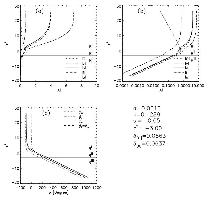
Figure 6: The example of a numerical DSAS for an isothermal atmosphere.

The frames $(a)$ and $(b)$ of Figure 6 show height dependences the modules of the wave component in the normal and logarithmic scales, accordingly. The frame $(c)$ of Figure 6 represents phases of the same components. In this case, we chose the height of transfer from an analytical solution to a numerical one equal to the critical height $z_{I}^{*}=z_{c}^{*}$. Any choice of $z_{I}^{*}>0$ leads to one and the same result. The parameters $s_{t}$ and $z_{t}^{*}$ height corresponding to it are given in the right lower quadrant in Figure 6. Solving a Cauchy problem in the reverse order from the height $z_{t}^{*}$ of Case II, all the height dependences are reproduced with very good acuracy in the region $I\cup II$. We do not give results of these tests because they coincide with the results of Figure 6. Figure 6 clearly convinces of sufficient smoothness of the wave solution in all its components. The measures of the discontinuity of the wave components $\Theta$ and $n$ at the height $z_{t}^{*}$ are displayed in the right lower quadrant in Figure 6. The notation $\delta_{[x]}$ denotes a value

$$\delta_{[x]}=2\frac{|X(+z_{t}^{*})-X(-z_{t}^{*})|}{|X(+z_{t}^{*})+X(-z_{t}^{*})|}.$$ (61)

As we expected, the values of these quantities are small and have the order of $s_{t}$.

Test B:

We carried out a test based on the fact that the analytical solution of Eq. (45) gives us a ready solution in the region $I$. We used this solution for setting the Cauchy problem in region $II$. We do not give a corresponding DSAS because it is visually identical with what was given in Figure 6. But in this case, we got some better measures of the discontinuity of a solution: $\delta_{[\Theta]}=0.0272$; $\delta_{[n]}=0.0264$.

Test C:

In the region $II\cup III$ we do not have the possibility of calculating a wave solution in an analytical form because of the difficulties caused by formal divergence of the series of the hypergeometric functions in Eq. (45). We can use only the asymptotics of the analytical solution at $z^{*}\to-\infty$ for tests. Figure 7 presents the comparison results of our DSAS and the asymptotics of the analytical solution. We chose $\texttt{Re}\Theta_{ref}=\texttt{Re}\left(\Theta e^{-\frac{1}{2}z^{*}}\right)$ as a value to be tested (solid line).

Figure 7: The analysis of a numerical DSAS in the lower asymptotic region.

For the asymptotics of the analytical solution, $\texttt{Re}\Theta_{ref}$ is derived from Formulas (39a,b), (41) and (46): $\texttt{Re}\Theta_{ref}=\texttt{Re}(e^{-iqz^{*}}+Ke^{iqz^{*}})$ (a dashed line.) In our case, the complex coefficient $K$ is sufficiently small, $K=-0.0055-i0.0439$.

Especially for comparison, we made calculations both taking into account small dissipation in $III$ and without taking it into consideration in this region. Furthermore, we, also for comparison, used two values of $s_{t}$. The results are shown in different frames of Figure 7. The calculations for frames $(a)$, $(c)$, and $(b)$, $(d)$ are distinguished by the fact that $(a)$, $(c)$ in the region $III$ take small dissipation into account in accordance with (15)-(19); $(b)$, $(d)$, the dissipationless approximation (3), (12)-(14). Frames $(a)$ and $(b)$ of Figure 7 give results for the cases with the least value $s_{t}$, $s_{t}=0.05$; frames $(c)$ and $(d)$, with a large value of the parameter $s_{t}$, $s_{t}=0.2$. In all cases, we clearly see that the numerical DSAS coincides with the analytical one up phase. Comparing $(a)$ and $(b)$, one can find only hardly noticeable advantage of result $(a)$. We can see more clearly a positive effect of taking small dissipation into account in region $III$ in Frame $(c)$ in comparison to $(d)$. The solution discontinuity indices most clearly show advantage of taking small dissipation into account:
the frame $(a)$ of Figure 7 – $\delta_{[\Theta]}=0.0272,\ \delta_{[n]}=0.0264$;
the frame $(b)$ of Figure 7 – $\delta_{[\Theta]}=0.1245,\ \delta_{[n]}=0.1200$;
the frame $(c)$ of Figure 7 – $\delta_{[\Theta]}=0.3760,\ \delta_{[n]}=0.3400$;
the frame $(d)$ of Figure 7 – $\delta_{[\Theta]}=0.4792,\ \delta_{[n]}=0.4408$.
The last equalities convince us of appropriateness of our small dissipation correction even at the least allowed values of the parameter $s_{t}$ and sufficiency of $0.05$ value for $s_{t}$ as well.

6 DSAS for a non-isothermal atmosphere

We used the model of the atmosphere introduced in Section 3.2.1 with the height distribution of undisturbed temperature shown in Figure 1. The calculation is carried out for the period $T=90.84\ min$ and horizontal wavelength $\lambda_{hor}=1365\ km$. The selected wave parameters $T$ and $\lambda_{hor}$ correspond to the dimensionless $\sigma$ and $k$ used in tests in the isothermal model. The following condition is used to norm the solution: $\texttt{Max}(\sqrt{v_{x}^{2}+v_{z}^{2}})=50\ m/sec$. The calculation results are shown in Figure 8. They clearly convince of sufficient smoothness of DSAS in all its components at the height of $z_{t}$. The discontinuity indices $\delta_{[\Theta]}=0.129,\ \delta_{[n]}=0.091$, approximately $5$ times higher than in an isothermal case, but remain sufficiently small. In the upper atmosphere above $z_{c}$, height dependences of the solution components are close in their nature to dependences of the isothermal model. As in the case of the isothermal model, we compare the received solution to the solution of the dissipationless problem. To do so, we solve the Cauchy problem for Eqs. (3), (12), (13) in the reverse direction from the Earth to the height of $z_{c}$. We do not show the received solution due to its too small graphical difference from the solution in Figure 8.

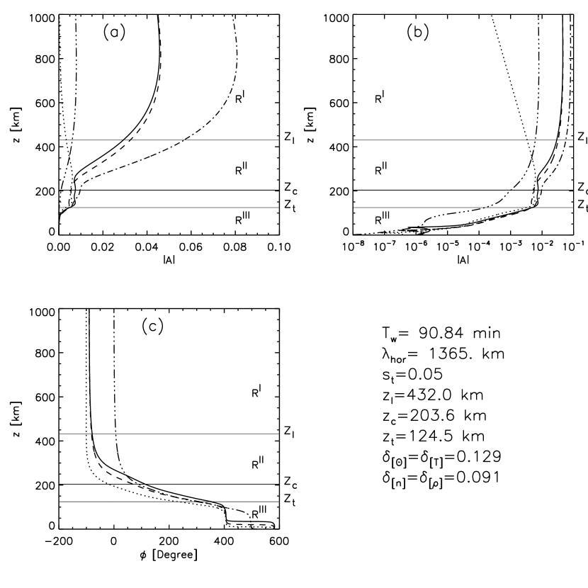
Figure 8: The example of a DSAS for a non-isothermal atmosphere.

7 Green’s matrix with DSAS (extended)

As it is well known, the problem on evolution of disturbance from some source can be solved without consideration of dissipation, using the $2\times 2$ Green’s matrix. However, the dissipationless solution has the disadvantage that it cannot adequately reflect the height structure in the upper atmospheric layers; therefore, one should use a higher order problem than the second one there. But one can achieve the goal of a height-structure description in the upper atmosphere and retain the formalism of the second-order problem to a significant extent at the same time. It is possible to do this in that case when, as it mainly occurs in the atmosphere, a source of disturbance is not too high, so that it does not enter the region of strong dissipation. For the problem on evolution of disturbance from some source with consideration of dissipation we will introduce the $2\times 2$ Green’s modified matrix, which we will call extended Green’s matrix. Let us start with the Green’s matrix for the weakly dissipative problem. The inhomogeneous weakly dissipative problem can be written in the form

$$\left(\begin{array}[]{c}p\\ v_{z}\end{array}\right)^{\prime}=\left(\begin{array}[]{cc}\tilde{a}_{11}&\tilde{a}_{12}\\ \tilde{a}_{21}&\tilde{a}_{22}\end{array}\right)\left(\begin{array}[]{c}p\\ v_{z}\end{array}\right)+\left(\begin{array}[]{c}f_{p}\\ f_{v}\end{array}\right).$$ (62)

The homogeneous part of (62) is got in Section 2 (19), the functions $\left(\begin{array}[]{c}f_{p}\\ f_{v}\end{array}\right)$ describe a source. They have zero values above $z_{max}$. Eqs. (62) is a second-order problem, and the corresponding Green’s matrix has the order $2\times 2$. For it construction $F^{u}=(p^{u},v_{z}^{u})$, we will use notations : is the weakly dissipative solution satisfying the upper boundary condition ( the upper solution); $F^{l}=(p^{l},v_{z}^{l})$, the weakly dissipative solution satisfying the lower boundary condition ( the lower solution). For the region $z<a$, where $a>z_{t}$, the Green’s function can be written in the form:

$$\begin{array}[]{l}G_{11}=\frac{1}{W(z^{\prime})}\times\left\{\begin{array}[]{c}p^{u}(z)v_{z}^{l}(z^{\prime}),\ 0<z^{\prime}<z\\ p^{l}(z)v_{z}^{u}(z^{\prime}),\ z<z^{\prime}<a\end{array}\right.;\\ G_{12}=\frac{1}{W(z^{\prime})}\times\left\{\begin{array}[]{c}v_{z}^{u}(z)v_{z}^{l}(z^{\prime}),\ 0<z^{\prime}<z\\ v_{z}^{l}(z)v_{z}^{u}(z^{\prime}),\ z<z^{\prime}<a\end{array}\right.;\\ G_{21}=\frac{-1}{W(z^{\prime})}\times\left\{\begin{array}[]{c}p^{u}(z)p^{l}(z^{\prime}),\ 0<z^{\prime}<z\\ p^{l}(z)p^{u}(z^{\prime}),\ z<z^{\prime}<a\end{array}\right.;\\ G_{22}=\frac{-1}{W(z^{\prime})}\times\left\{\begin{array}[]{c}v_{z}^{u}(z)p^{l}(z^{\prime}),\ 0<z^{\prime}<z\\ v_{z}^{l}(z)p^{u}(z^{\prime}),\ z<z^{\prime}<a\end{array}\right..\end{array}$$ (63)

Here $W(z^{\prime})=v_{z}^{l}()z^{\prime})p^{u}(z^{\prime})-v_{z}^{u}()z^{\prime})p^{l}(z^{\prime})$ The solution of (62) is

$$\begin{array}[]{l}p(z)=\int\limits_{0}^{a}G_{11}(z,z^{\prime})f_{p}(z^{\prime})dz^{\prime}+\int\limits_{0}^{a}G_{21}(z,z^{\prime})f_{v}(z^{\prime})dz^{\prime},\\ v_{z}(z)=\int\limits_{0}^{a}G_{12}(z,z^{\prime})f_{p}(z^{\prime})dz^{\prime}+\int\limits_{0}^{a}G_{22}(z,z^{\prime})f_{v}(z^{\prime})dz^{\prime}\end{array}$$ (64)

It is clear that, if we use DSAS as the upper solution then we will get a solution of the dissipation problem, the homogeneous part of which is given by formulae (3), (8), (9) and the source is from (62). The disturbance in the upper atmospheric layers is:
$F(z)=F^{u}(z)\int\limits_{0}^{z_{max}}\frac{1}{W(z^{\prime})}[v_{z}^{l}(z^{\prime})f_{p}(z^{\prime})-p^{l}(z^{\prime})f_{v}(z^{\prime})]dz^{\prime}$

Conclusion

In this paper, we proposed a method for obtaining a wave solution above a source for the real atmosphere (DSAS). The method of construction of DSAS was successfully tested with the everywhere isothermal atmosphere model.

The most essential elements of the test are: calculation of jumps at the matching point to have demonstrated their sufficient smallness and comparison of the numerical solution with an asymptotics of an analytical solution in the region of small dissipation to have demonstrated their coincidence. We have also given the results of DSAS calculations for a real non-isothermal atmosphere.

DSAS itself describes height structure of disturbance above any source provided that it is in the lower part of the atmosphere. In this paper, it is shown that one can construct an expanded Green’s matrix $2\times 2$ with use of DSAS and a solution for the lower weekly dissipative part of the atmosphere, which, as we have shown, can be found analogously to the dissipationless one. The expanded Green’s matrix let us to find the disturbance produced by some source in the all height ranges. erewith, the DSAS amplitude is completely determined.

The specific feature of DSAS is describing of dissipative tail, formally indefinitely extended to the isothermal part of the atmosphere. The essential circumstance is that the exponential increase of wave values, relative to background, is changed by their slow decrease, due to dissipation effect. This allows the wave to remain in the frames of the linear description, in whole range of its existence, on condition that its amplitude in the lower part of the atmosphere is sufficiently small. It is important that the method proposed has prospects of the further development in the framework of a more complex model of the atmosphere. In particularly, including vertically stratified wind is possible. The necessary equations for such models are written in this paper. It is also possible to take more complete wave dissipation into account, including not only heat conductivity but viscosity as well.

In this case, the part of DSAS in the upper height range, where dissipation is not small, is described, as we shown in this paper, by the system of six ODEs. Respectively, this system has six independent solutions. For the asymptotic isothermal region, the solutions taking into account both heat conductivity and viscosity were obtain in Rudenko (1994b). A combination of three such isothermal solutions will satisfy the upper boundary condition. The way to ensure sufficient smoothness of DSAS is the same as in this paper.

Appendix A

$t_{11}=\frac{\Gamma\left(-2k\right)\Gamma\left(\frac{1}{2}+\alpha-k\right)\Gamma\left(\frac{1}{2}-\alpha-k\right)\Gamma\left(\frac{1}{2}+k-iq\right)}{\Gamma\left(\frac{1}{2}-iq-k\right)}e^{i\frac{\pi}{2}k}$,

$t_{12}=\frac{\Gamma\left(2k\right)\Gamma\left(\frac{1}{2}+\alpha+k\right)\Gamma\left(\frac{1}{2}-\alpha+k\right)\Gamma\left(\frac{1}{2}-k-iq\right)}{\Gamma\left(\frac{1}{2}-iq+k\right)}e^{-i\frac{\pi}{2}k}$,

$t_{13}=\frac{\Gamma\left(k-\frac{1}{2}-\alpha\right)\Gamma\left(-k-\frac{1}{2}-\alpha\right)\Gamma\left(-2\alpha\right)\Gamma\left(1+\alpha-iq\right)}{\Gamma\left(-iq-\alpha\right)}e^{i\frac{\pi}{2}\left(\frac{1}{2}+\alpha\right)}$,

$t_{14}=\frac{\Gamma\left(k-\frac{1}{2}+\alpha\right)\Gamma\left(-k-\frac{1}{2}+\alpha\right)\Gamma\left(2\alpha\right)\Gamma\left(1-\alpha-iq\right)}{\Gamma\left(-iq+\alpha\right)}e^{i\frac{\pi}{2}\left(\frac{1}{2}-\alpha\right)}$,

$t_{21}=\frac{\Gamma\left(-2k\right)\Gamma\left(\frac{1}{2}+\alpha-k\right)\Gamma\left(\frac{1}{2}-\alpha-k\right)\Gamma\left(\frac{1}{2}+k+iq\right)}{\Gamma\left(\frac{1}{2}+iq-k\right)}e^{i\frac{\pi}{2}k}$,

$t_{22}=\frac{\Gamma\left(2k\right)\Gamma\left(\frac{1}{2}+\alpha+k\right)\Gamma\left(\frac{1}{2}-\alpha+k\right)\Gamma\left(\frac{1}{2}-k+iq\right)}{\Gamma\left(\frac{1}{2}+iq+k\right)}e^{-i\frac{\pi}{2}k}$,

$t_{23}=\frac{\Gamma\left(k-\frac{1}{2}-\alpha\right)\Gamma\left(-k-\frac{1}{2}-\alpha\right)\Gamma\left(-2\alpha\right)\Gamma\left(1+\alpha+iq\right)}{\Gamma\left(iq-\alpha\right)}e^{i\frac{\pi}{2}\left(\frac{1}{2}+\alpha\right)}$,

$t_{24}=\frac{\Gamma\left(k-\frac{1}{2}+\alpha\right)\Gamma\left(-k-\frac{1}{2}+\alpha\right)\Gamma\left(2\alpha\right)\Gamma\left(1-\alpha+iq\right)}{\Gamma\left(iq+\alpha\right)}e^{i\frac{\pi}{2}\left(\frac{1}{2}-\alpha\right)}$,

$t_{31}=\frac{\Gamma\left(-2k\right)\Gamma\left(\frac{1}{2}+\alpha-k\right)\Gamma\left(\frac{1}{2}-\alpha-k\right)}{\Gamma\left(\frac{1}{2}+iq-k\right)\Gamma\left(\frac{1}{2}-iq-k\right)}e^{-i\frac{\pi}{2}k}$,

$t_{32}=\frac{\Gamma\left(2k\right)\Gamma\left(\frac{1}{2}+\alpha+k\right)\Gamma\left(\frac{1}{2}-\alpha+k\right)}{\Gamma\left(\frac{1}{2}+iq+k\right)\Gamma\left(\frac{1}{2}-iq+k\right)}e^{i\frac{\pi}{2}k}$,

$t_{33}=\frac{\Gamma\left(k-\frac{1}{2}-\alpha\right)\Gamma\left(-k-\frac{1}{2}-\alpha\right)\Gamma\left(-2\alpha\right)}{\Gamma\left(iq-\alpha\right)\Gamma\left(-iq-\alpha\right)}e^{-i\frac{\pi}{2}\left(\frac{1}{2}+\alpha\right)}$,

$t_{34}=\frac{\Gamma\left(k-\frac{1}{2}+\alpha\right)\Gamma\left(-k-\frac{1}{2}+\alpha\right)\Gamma\left(2\alpha\right)}{\Gamma\left(iq+\alpha\right)\Gamma\left(-iq+\alpha\right)}e^{-i\frac{\pi}{2}\left(\frac{1}{2}-\alpha\right)}$.

References

- Afraimovich at. al. (2001) Afraimovich, E. L., Kosogorov, E. A., Lesyuta, O. S., Ushakov, I. I., Yakovets Network, A. F. 2001. Geomagnetic control of the spectrum of traveling ionospheric disturbances based on data from a global GPS network. Annales Geophysicae, Volume 19, Issue 7, 2001, pp.723-731, doi: 10.5194/angeo-19-723-2001.
- Akmaev (2001) Akmaev, R. A. 2001. Simulation of large-scale dynamics in the mesosphere and lower thermosphere with the Doppler-spread parameterization of gravity waves: 2. Eddy mixing and the diurnal tide. Journal of Geophysical Research: Atmospheres, Volume 106, Issue D1, pp. 1205-1213, doi: 10.1029/2000JD900519.
- Angelatsi and Forbes (2002) Angelatsi Coll, M.; Forbes, J. M. 2002. Nonlinear interactions in the upper atmosphere: The s = 1 and s = 3 nonmigrating semidiurnal tides. Journal of Geophysical Research (Space Physics), Volume 107, Issue A8, pp. SIA 3-1, CiteID 1157, DOI 10.1029/2001JA900179.
- Fesen (1995) Fesen, C. G. 1995. Tidal effects on the thermosphere. Surveys in Geophysics, Volume 13, Issue 3, pp.269-295, doi: 10.1007/BF02125771.
- Forbes and Garrett (1979) Forbes, J. M.; Garrett, H. B. 1979. Theoretical studies of atmospheric tides. Reviews of Geophysics and Space Physics, vol. 17, Nov. 1979, p. 1951-1981, doi: 10.1029/RG017i008p01951.
- Francis (1973a) Francis, S. H. 1973a. Acoustic-gravity modes and large-scale traveling ionospheric disturbances of a realistic, dissipative atmosphere, J.Geophys. Res., 78, 2278.
- Francis (1973b) Francis, S. H. 1973b. Lower-atmospheric gravity modes and their relation to mediumscale traveling ionospheric disturbances, J. Geophys. Res., 78, 8289-8295.
- Gavrilov (1995) Gavrilov, N. M. 1995. Distributions of the intensity of ion temperature perturbations in the thermosphere. Journal of Geophysical Research, Volume 100, Issue A12, p. 23835-23844, doi: 10.1029/95JA01927, 1995.
- Gavrilov, and Kshevetskii (2014) Gavrilov, N. M.; Kshevetskii, S. P. 2014. Numerical modeling of the propagation of nonlinear acoustic-gravity waves in the middle and upper atmosphere. Izvestiya, Atmospheric and Oceanic Physics, Volume 50, Issue 1, pp.66-72.
- Gossard and Hooke (1975) Gossard, E. E. and Hooke, W. H. 1975. Waves in the Atmosphere, Elsevier Scientific Publishing Company, New York, 456 pp.
- Grigor’ev (1999) Grigor’ev, G. I. 1999. Acoustic-gravity waves in the earth’s atmosphere (review). Radiophysics and Quantum Electronics, Volume 42, Issue 1, pp.1-21, doi: 10.1007/BF02677636.
- Heale at. al. (2014) Heale, C. J., Snively, J. B., Hickey, M. P., Ali, C. J. 2014 Thermospheric dissipation of upward propagating gravity wave packets. Journal of Geophysical Research: Space Physics, Volume 119, Issue 5, pp. 3857-3872, doi: 10.1002/2013JA019387.
- Hedlin at. al. (2014) Hedlin, Michael A. H.; Drob, Douglas P. 2014. Statistical characterization of atmospheric gravity waves by seismoacoustic observations. Journal of Geophysical Research: Atmospheres, Volume 119, Issue 9, pp. 5345-5363, doi: 10.1002/2013JD021304.
- Hickey et. al. (1997) Hickey, M. P., Walterscheid, R. L., Taylor, M. J., Ward, W., Schubert, G.,Zhou, Q., Garcia, F., Kelly, M. C., Shepherd, G. G. 1997. Numericalsimulations of gravity waves imaged over Arecibo during the 10-dayJanuary, campaign. J. Geophys. Res. 102 (A6), 11475-11490.
- Hickey et. al. (1998) Hickey, M. P., Taylor, M. J., Gardner, C. S., Gibbons, C. R. 1998. Full-wavemodeling of small-scale gravity waves using Airborne Lidar andObservations of the Hawaiian Airglow (ALOHA-93) O(1S) images andcoincident Na wind/temperature lidar measurements. J. Geophys. Res.103 (D6), 6439-6454.
- Hines (1960) Hines, C. O. 1960. Internal atmospheric gravity waves at ionospheric heights, Can. J. Phys., 38, 1441-1481.
- Idrus et. al. (2013) Idrus, Intan Izafina; Abdullah, Mardina; Hasbi, Alina Marie; Husin, Asnawi; Yatim, Baharuddin. 2013. Large-scale traveling ionospheric disturbances observed using GPS receivers over high-latitude and equatorial regions. Journal of Atmospheric and Solar-Terrestrial Physics, Volume 102, p. 321-328, doi: 10.1016/j.jastp.2013.06.014.
- Kshevetskii and Gavrilov (2005) Kshevetskii S. P., Gavrilov N. M. 2005. Vertical propagation, breaking and effects of nonlineargravity waves in the atmosphere. Journal ofAtmospheric and Solar-Terrestrial Physics. V.67. P. 1014-1030.
- Lindzen (1970) Lindzen, R. S. 1970. Internal gravity waves in atmospheres with realistic dissipation and temperature part I. Mathematical development and propagation of waves into the thermosphere, Geophysical & Astrophysical Fluid Dynamics, vol. 1, issue 3, pp. 303-355.
- Lindzen (1971) Lindzen, R. S. 1971. Internal gravity waves in atmospheres with realistic dissipation and temperature part III. Daily variations in the thermosphere, Geophysical and Astrophysical Fluid Dynamics, 1971, vol. 2, Issue 1, pp.89-121
- Lindzen and Blake (1971) Lindzen, R. S. and Blake, D. 1971. Internal gravity waves in atmospheres with realistic dissipation and temperature part II. Thermal tides excited below the mesopause, Geophysical Fluid Dynamics, 2:1, 31-61, DOI: 10.1080/03091927108236051.
- Lindzen (1981) Lindzen R. S. Turbulence and stress owing to gravity wave and tidal breakdown, J. Gephys. Res. V. 86. P. 9707-9714.
- Luke (1975) Luke, Y. L. 1975. Mathematical functions and their approximations. Academic Press. 584.
- Lyons and Yanowitch (1974) Lyons, P., Yanowitch, M. 1974. Vertical oscillatins in a viscous and thermally conducting isotermal atmosphere. J. Fluid. Mech.
- Ostashev (1997) Ostashev, V. E. 1997. Acoustics in Moving Inhomogeneous Media. E & FN Spon, London 259p.
- Pierce and Posey (1970) Pierce A. D., Posey J. W. 1970. Theoretical predictions of acoustic-gravity pressure waveforms generated by large explosions in the atmosphere, Air Force Camb. Res. Lab., AFCRL-70-0134.
- Pierce at. al. (1971) Pierce A. D., Posey J. W., Illiff E. F. 1971. Variation of nuclear explosion generated acoustic-gravity wave forms with burst height and with energy yield, J. Geophys. Res., 76(21), 5025-5041.
- Ponomarev et. al. (2006) Ponomarev, E. A., Rudenko, G. V., Sorokin, A. G., Dmitrienko, I. S., Lobycheva, I. Yu., Baryshnikov, A. K. 2006. Using the normal-mode method of probing the infrasonic propagation for purposes of the comprehensive nuclear-test-ban treaty. Journal of Atmospheric and Solar-Terrestrial Physics 68, 599-614.
- Rudenko (1994a) Rudenko, G. V. 1994a. Linear oscillatins in a viscous and heat-conducting isothermal atmosphere: Part 1. Atmospheric and Oceanic Physics. 30, No 2, 134-143.
- Rudenko (1994b) Rudenko, G. V. 1994b. Linear oscillatins in a viscous and heat-conducting isothermal atmosphere: Part 2. Atmospheric and Oceanic Physics. 30, No 2, 144-152.
- Shibata and Okuzawa (1983) Shibata, T., Okuzawa, T. 1983. Horizontal velocity dispersion of medium-scale travelling ionospheric disturbances in the F-region. Journal of Atmospheric and Terrestrial Physics (ISSN 0021-9169), vol. 45, Feb.-Mar., p. 149-159.
- Snively and Pasko (2003) Snively, J. B., Pasko, V. P. 2003. Breaking of thunderstorm-generated gravity waves as a source of short-period ducted waves at mesopause altitudes. Geophys. Res. Lett. 30 (24), 2254, doi:10.1029/2003GL018436.
- Snively and Pasko (2005) Snively, J. B., Pasko, V. P. 2005. Antiphase OH and OI airglow emissions induced by a short-period ducted gravity wave. Geophys. Res. Lett. 32, L08808, doi:10.1029/2004GL022221.
- Snively et. al (2007) Snively, J. B., Pasko, V. P., Taylor, M. J., Hocking, W. K. 2007. Doppler ductingof short-period gravity waves by midlatitude tidal wind structure. J. Geophys. Res. 112, A03304, doi:10.1029/2006JA011895.
- Vadas (2005) Vadas, S. L., Fritts, D. C. 2005. Thermospheric responses to gravity waves: Influences of increasing viscosity and thermal diffusivity. J. Geophys. Res., 110, D15103, doi:10.1029/2004JD005574.
- Vadas and Liu (2009) Vadas, Sharon L., Liu, Han-li. 2009. Generation of large-scale gravity waves and neutral winds in the thermosphere from the dissipation of convectively generated gravity waves. Journal of Geophysical Research, Volume 114, Issue A10, CiteID A10310, doi: 10.1029/2009JA014108.
- Vadas and Nicolls (2012) Vadas, S. L., Nicolls, M. J. 2012. The phases and amplitudes of gravity waves propagating and dissipating in the thermosphere: Theory. Journal of Geophysical Research, Volume 117, Issue A5, CiteID A05322, doi: 10.1029/2011JA017426.
- Walterscheid and Schubert (1990) Walterscheid, R.L., Schubert, G. 1990. Nonlinear evolution of an upwardpropagating gravity wave: overturning, convection, transience andturbulence. J. Atmos. Sci. 47 (1), 101-125.
- Walterscheid at. al. (2001) Walterscheid, R. L., Schubert, G., Brinkman, D. G. 2001. Small-scale gravitywaves in the upper mesosphere and lower thermosphere generated by deep tropical convection. J. Geophys. Res. 106 (D23), 31825-31832.
- Yu and Hickey (2007a) Yu, Y., Hickey, M. P. 2007a. Time-resolved ducting of atmospheric acousticgravitywaves by analysis of the vertical energy flux. Geophys. Res.Lett. 34, L02821, doi:10.1029/2006GL028299.
- Yu and Hickey (2007b) Yu, Y., Hickey, M. P. 2007b. Numerical modeling of a gravity wave packet ductedby the thermal structure of the atmosphere. J. Geophys. Res. 112, A06308, doi:10.1029/2006JA012092,.
- Yu and Hickey (2007c) Yu, Y., Hickey, M. P. 2007c. Simulated ducting of high-frequency atmosphericgravity waves in the presence of background winds. Geophys. Res. Lett. 34, L11103, doi:10.1029/2007GL029591.
- Yu at. al. (2009) Yu, Y., Hickey, M. P., Liu, Y. 2009. A numerical model characterizing internal gravity wave propagation into the upper atmosphere.Advances in Space Research, Volume 44, Issue 7, p. 836-846.,doi: 10.1016/j.asr.2009.05.014.
- Yanowitch (1967a) Yanowitch, M. 1967a. Effect of viscosity on oscillatins of an isotermal atmosphere. Can. J. Phys. 45, 2003-2008.
- Yanowitch (1967b) Yanowitch, M. 1967b. Effect of viscosity on gravity waves and apper boundary conditions. J. Fluid. Mech. 29, Part 2, 209-231.