Differential Rotation in Solar Convective Dynamo Simulations

Abstract

We carry out a magneto-hydrodynamic (MHD) simulation of convective dynamo in the rotating solar convective envelope driven by the solar radiative diffusive heat flux. The simulation is similar to that reported in Fan & Fang (2014) but with further reduced viscosity and magnetic diffusion. The resulting convective dynamo produces a large scale mean field that exhibits similar irregular cyclic behavior and polarity reversals, and self-consistently maintains a solar-like differential rotation. The main driver for the solar-like differential rotation (with faster rotating equator) is a net outward transport of angular momentum away from the rotation axis by the Reynolds stress, and we found that this transport is enhanced with reduced viscosity and magnetic diffusion.

1 Introduction

Significant advances have been made in recent years in global-scale fully dynamic three-dimensional convective dynamo simulations of the solar/stellar convective envelopes to reproduce some of the basic features of the Sun’s large-scale cyclic magnetic field (e.g. Ghizaru et al., 2010; Racine et al., 2011; Käpylä et al., 2012; Nelson et al., 2013; Fan & Fang, 2014; Augustson et al., 2015; Hotta et al., 2015). It has also been found that the presence of the dynamo generated magnetic fields may be important in the self-consistent maintenance of the solar-like differential rotation with the equator rotating faster than the poles (e.g. Fan & Fang, 2014; Karak et al., 2015; Mabuchi et al., 2015; Simitev et al., 2015). It has been shown that if the buoyancy driving of convection becomes too strong compared to the Coriolis force such that the convection is no-longer rotationally constrained, as measured by the Rossby number $R_{o}\equiv v/\Omega L$ becoming significantly greater than 1, where $v$ and $L$ are the characteristic convective speed and length scale and $\Omega$ is the angular rotation rate, anti-solar differential rotation (faster rotating poles) develops (e.g. Matt et al., 2011; Gastine et al., 2013; Guerrero et al., 2013). Fan & Fang (2014) found that the dynamo generated magnetic field can have the effect of an enhanced viscosity that suppresses convection to keep it rotationally constrained such that the Reynolds stress generated by the convection drives a solar-like differential rotation, while in the corresponding hydrodynamic case in the absense of the magnetic field the differential rotation becomes anti-solar. Here we continue to investigate the dynamic reaction of the magnetic field by further reducing the viscosity and the magnetic diffusivity in the convective dynamo simulation from that of Fan & Fang (2014). We find that the self-consistent maintenance of the solar-like differential rotation remains robust, and the resulting large-scale mean magnetic field also shows a similar irregular cyclic behavior. With reduced viscosity and magnetic diffusivity, we find the tendency of an enhanced magnetic energy, and a reduction of the kinetic energy of convection on the larger scales. As a result the outward transport (away from the rotation axis) of angular momentum by the Reynolds stress is further increased, balanced by an increased inward transport by the magnetic stress, with the transport by the viscous stress reduced to a negligible level.

2 Description of the Numerical Simulations

The setup of the numerical simulation is the same as that described in Fan & Fang (2014, hereafter FF) except the specification of the kinetic viscosity $\nu$ and magnetic diffusivity $\eta$. Here for the clarity of this paper we reiterate the key features of the numerical model. We solve the following anelastic MHD equations using a finite-difference spherical anelastic MHD code (Fan et al., 2013):

$$\nabla\cdot(\rho_{0}{\bf v})=0,$$ (1)

$$\rho_{0}\left[\frac{\partial{\bf v}}{\partial t}+({\bf v}\cdot\nabla){\bf v}\right]=2\rho_{0}{\bf v}\times{\bf\Omega}_{0}-\nabla p_{1}+\rho_{1}{\bf g}+\frac{1}{4\pi}(\nabla\times{\bf B})\times{\bf B}+\nabla\cdot{\cal D},$$ (2)

$$\rho_{0}T_{0}\left[\frac{\partial s_{1}}{\partial t}+({\bf v}\cdot\nabla)(s_{0}+s_{1})\right] = \nabla\cdot(K\rho_{0}T_{0}\nabla s_{1})$$ (3)

$$-({\cal D}\cdot\nabla)\cdot{\bf v}+\frac{1}{4\pi}\eta(\nabla\times{\bf B})^{2}$$

$$-\nabla\cdot{\bf F}_{\rm rad},$$

$$\nabla\cdot{\bf B}=0,$$ (4)

$$\frac{\partial{\bf B}}{\partial t}=\nabla\times({\bf v}\times{\bf B})-\nabla\times(\eta\nabla\times{\bf B}),$$ (5)

$$\frac{\rho_{1}}{\rho_{0}}=\frac{p_{1}}{p_{0}}-\frac{T_{1}}{T_{0}},$$ (6)

$$\frac{s_{1}}{c_{p}}=\frac{T_{1}}{T_{0}}-\frac{\gamma-1}{\gamma}\frac{p_{1}}{p_{0}},$$ (7)

where $s_{0}(r)$, $p_{0}(r)$, $\rho_{0}(r)$, $T_{0}(r)$, and ${\bf g}=-g_{0}(r){\hat{\bf r}}$ are the profiles of entropy, pressure, density, temperature, and the gravitational acceleration of a time-independent, reference state of hydrostatic equilibrium and nearly adiabatic stratification, $c_{p}$ is the specific heat capacity at constant pressure, $\gamma$ is the ratio of specific heats, ${\bf v}$, ${\bf B}$, $s_{1}$, $p_{1}$, $\rho_{1}$, and $T_{1}$ are the dependent velocity field, magnetic field, entropy, pressure, density, and temperature to be solved that describe the changes from the reference state. Also in the above equations, ${\bf\Omega}_{0}$ with $\Omega_{0}=2.7\times 10^{-6}{\rm rad}\;{\rm s}^{-1}$, denotes the solid body rotation rate of the Sun which is used as the frame of reference. ${\cal D}$ denotes the viscous stress tensor: ${\cal D}_{ij}=\rho_{0}\nu\left[S_{ij}-(2/3)(\nabla\cdot{\bf v})\delta_{ij}\right]$, where $\nu$ is the kinematic viscosity, $\delta_{ij}$ is the unit tensor, and $S_{ij}$ is the strain rate tensor given by the following in spherical polar coordinates:

$$S_{rr}=2\frac{\partial v_{r}}{\partial r}$$ (8)

$$S_{\theta\theta}=\frac{2}{r}\frac{\partial v_{\theta}}{\partial\theta}+\frac{2v_{r}}{r}$$ (9)

$$S_{\phi\phi}=\frac{2}{r\sin\theta}\frac{\partial v_{\phi}}{\partial\phi}+\frac{2v_{r}}{r}+\frac{2v_{\theta}}{r\sin\theta}\cos\theta$$ (10)

$$S_{r\theta}=S_{\theta r}=\frac{1}{r}\frac{\partial v_{r}}{\partial\theta}+r\frac{\partial}{\partial r}\left(\frac{v_{\theta}}{r}\right)$$ (11)

$$S_{\theta\phi}=S_{\phi\theta}=\frac{1}{r\sin\theta}\frac{\partial v_{\theta}}{\partial\phi}+\frac{\sin\theta}{r}\frac{\partial}{\partial\theta}\left(\frac{v_{\phi}}{\sin\theta}\right)$$ (12)

$$S_{\phi r}=S_{r\phi}=\frac{1}{r\sin\theta}\frac{\partial v_{r}}{\partial\phi}+r\frac{\partial}{\partial r}\left(\frac{v_{\phi}}{r}\right).$$ (13)

$K$ denotes the thermal diffusivity, and $\eta$ is the magnetic diffusivity. In equation (3),

$${\bf F_{\rm rad}}=-\frac{16\sigma_{s}{T_{0}}^{3}}{3\kappa\rho_{0}}\frac{dT_{0}}{dr}\,{\hat{\bf r}}$$ (14)

is the radiative diffusive heat flux, where $\sigma_{s}$ is the Stefan-Boltzmann constant, $\kappa$ is the Rosseland mean opacity.

The simulation domain is a partial spherical shell where $r$ ranges from $0.722R_{\odot}$ (base of the solar convection zone) to $0.971R_{\odot}$ (about 20 Mm below the solar photosphere), $\theta$ (polar angle) ranges between $\pm 60^{\circ}$ latitudes, and $\phi$ spans the full azimuthal range of $0^{\circ}$ to $360^{\circ}$. The domain is resolved by a grid of $96(r)\times 512(\theta)\times 768(\phi)$. We use J. Christensen-Dalsgaard’s (JCD) solar model (Christensen-Dalsgaard et al., 1996) for the reference profiles of $T_{0}(r)$, $\rho_{0}(r)$, $p_{0}(r)$, $g_{0}(r)$ and assume $s_{0}(r)=0$. The heating $-\nabla\cdot{\bf F}_{\rm rad}$ in equation (3) due to the solar radiative diffusive heat flux given by the JCD model drives a radial gradient of $s_{1}$ that drives the convection. In FF, we set the thermal diffusivity $K=3\times 10^{13}\,{\rm cm}^{2}\,{\rm s}^{-1}$, the kinetic viscosity $\nu=10^{12}\,{\rm cm}^{2}\,{\rm s}^{-1}$, and the magnetic diffusivity $\eta=10^{12}\,{\rm cm}^{2}\,{\rm s}^{-1}$ at the top of the domain, and they all decrease with depth following a $1/\sqrt{\rho_{0}}$ profile. Here in this simulation, we keep the same thermal diffusivity $K$, but set $\nu$ and $\eta$ both to zero. Thus the explicit viscous and resistive terms in the above anelastic MHD equations become zero, but there are still numerical diffusions due to the upwinded, slope-limited evaluations of the fluxes in the advection terms and the electric field in the induction equation (Fan et al., 2013).

We use the same boundary and initial conditions as FF. The boundaries in $r$ and $\theta$ are non-penetrating and stress free for the velocity, perfect electric conducting walls for the magnetic field at the bottom and $\theta$ boundaries, and radial magnetic field at the top boundary. These ensure strict angular momentum conservation for the domain. We impose $\partial s_{1}/\partial r=0$ at the bottom boundary, $s_{1}=0$ at the top boundary, and $\partial s_{1}/\partial\theta=0$ at the $\theta$ boundaries. Thus the only energy flux coming into the domain is the solar radiative diffusive heat flux through the bottom, and the only energy flux coming out of the domain is the conductive heat flux due to the thermal diffusion at the top. A latitudinal gradient of entropy $s_{1}$ is also imposed at the lower boundary, corresponding to a pole to equator temperature gradient of about $6.8$ K, to represent the tachocline induced entropy variation that can break the Taylor-Proudman constraint in the convection zone (Rempel, 2005; Miesch et al., 2006). The initial state is an unstable thermal equilibrium with a super-adiabatic initial $\left<s_{1}\right>$ profile (with “$\left<\right>$” denoting horizontal averaging), where the thermal conductive heat flux together with the radiative diffusive heat flux carries the (constant) solar luminosity through the domain. We start with a small seed velocity and magnetic field and let the magneto-convection develop in the domain.

3 Results

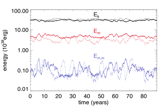
Figure 1: The variation of total kinetic energy $E_{k}$ (black curves), the total magnetic energy $E_{m}$ (red curves), and the azimuthally averaged mean magnetic energy $E_{\rm m,m}$ (blue curves) over a sample time span of 89 years of the statistically steady evolution from the present simulation (solid curves) and, in comparison, those from the dynamo simulation in FF (dotted curves)

Figure 1 shows the time sequences of the total kinetic energy $E_{\rm k}$, the total magnetic energy $E_{\rm m}$, and the azimuthally averaged mean magnetic energy $E_{\rm m,m}$ over a sample time span of about 89 years after the convective dynamo has reached statistically steady evolution (solid curves), in comparison to those obtained in FF (dashed curves). With reduced magnetic diffusivity and viscosity in the current convective dynamo simulation, we find that the total magnetic energy $E_{\rm m}$ is on average enhanced to about 1.51 times that of FF, while the total kinetic energy $E_{\rm k}$ is on average suppressed to about 0.91 of that in FF, and the mean (azimuthally averaged) magnetic energy $E_{\rm m,m}$ amplitude is very close to that of FF, although on average there is a statistically significant increase (at about the 3 sigma level) compared to FF. The ratio of the poloidal magnetic energy over the toroidal magnetic energy, $\int({B_{r}}^{2}+{B_{\theta}}^{2})dV/\int{B_{\phi}}^{2}dV$, is slightly increased, being $1.160\pm 0.001$ in the present case compared to $1.105\pm 0.001$ in FF.

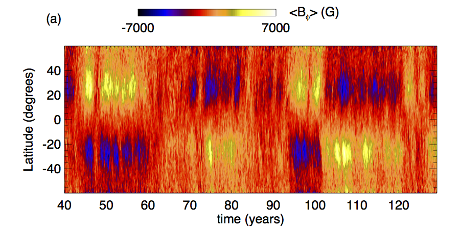
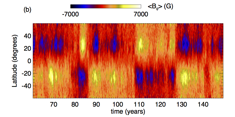
Figure 2: The latitude-time diagram of the (azimuthally averaged) mean toroidal magnetic field near the bottom of the convection zone for a sample time span of 89 years from the present convective dynamo simulation (panel a) compared to that of a same length of time span obtained from the convective dynamo simulation in FF (panel b).

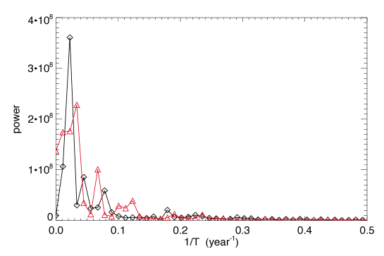
Figure 3: Frequency power spectrum obtained by carrying out Fourier analysis of the time sequence at each latitude in the latitude-time diagrams in Figure 2, and averaging over the latitudes. The black curve (red curve) is for the present case (FF case).

The large-scale mean (azimuthally averaged) toroidal magnetic field shows a irregular cyclic behavior with irregular polarity reversals, as can be seen in the latitude-time diagram of the mean toroidal magnetic field near the bottom of the convection zone (see Figure 2(a)), qualitatively similar to the result in FF (shown here in Figure 2(b)). By carrying out Fourier analysis of the time sequence at each latitude in the latitude-time diagrams in Figure 2, and averaging over the latitudes, we obtain the frequency power spectrum as shown in Figure 3 for the present case (black curve) and for FF (red curve). We see power peaks at periods of about 44.6 years, 22.3 years, 12.8 years, 5.6 years for the first 4 peaks in the present case. The second dominant peak is at the solar magnetic cycle period (about 22 years). For the FF case, we see power peaks at periods of about 29.8 years, 14.9 years, 8.1 years, and 5.3 years for the first 4 peaks, with the solar magnetic cycle period falls between the 2 most dominant peaks. The increase in the periods for the power peaks may be related to an increase in the magnetic diffusion time scales due to the reduction of the magnetic diffusivity in the present case.

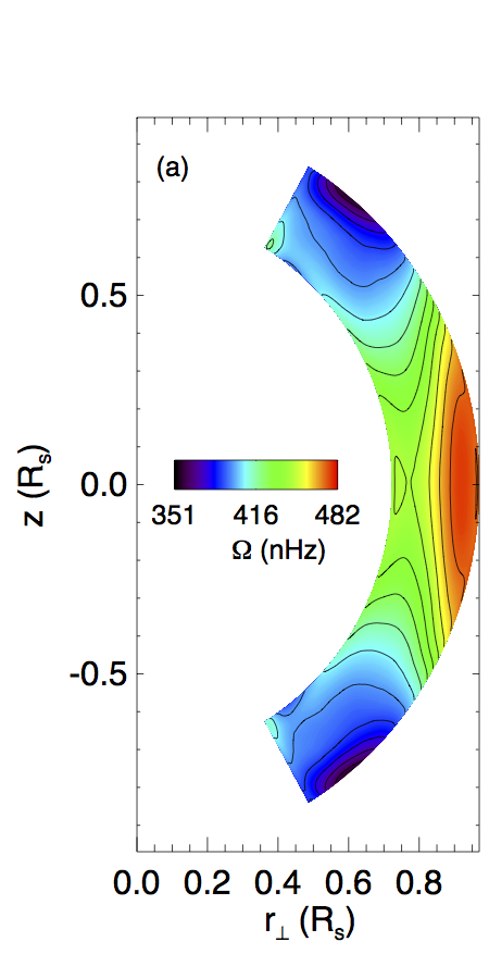
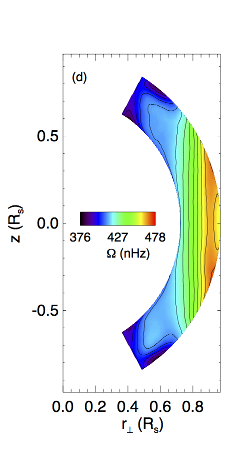
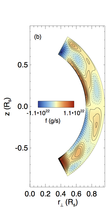
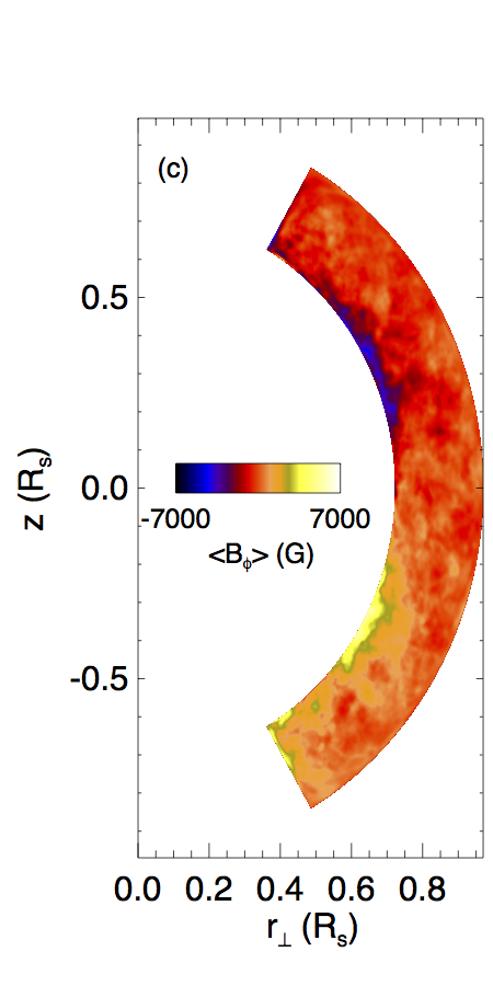
Figure 4: (a) The time and azimuthally averaged angular rotation rate, (b) time and azimuthally averaged meridional circulation mass flux $f$, where $\rho_{0}\left<{\bf v}_{m}\right>=\nabla\times[(f/r\sin\theta){\hat{\bf\phi}}]$, and $\left<{\bf v}_{m}\right>$ denotes the mean velocity in the meridional plane, (c) a snap shot of the azimuthally averaged toroidal magnetic field in the meridional plane, and (d) the time and azimuthally averaged agular rotation rate obtained if the latitudinal entropy gradient imposed at the bottom boundary of the convection zone is removed.

Figure 4 shows the time and azimuthally averaged angular rotation rate (panel (a)), the time and azimuthally averaged meridional circulation mass flux (panel (b)), and a snapshot of the azimuthally averaged toroidal magnetic field in the meridional plane (panel (c)) resulting from the present simualation. The differential rotation profile self-consistently maintained by the convective dynamo is solar-like (e.g. Thompson et al., 2003), with a faster rotation rate at the outer equatorial region than that at the polar region by about 30% of the mean rotation rate, and with the isorotation contours bending towards conical shaped in the mid-latitude zone. In the high and mid latitude region and at deeper depths, the iso-rotation contours bend toward horizontal to show a radial gradient of differential rotation, similar to the observed solar differential rotation profile. Figure 4(d) shows the resulting profile of differential rotation if the imposed latitude gradient of entropy at the base of the of the convection zone is removed. We see that the iso-rotational contours become more cylindrical, and the tendency for them to turn towards conical shaped in the mid latitude region is significantly diminished. This confirms the role of the tachocline induced entropy variation at the bottom of the convection zone that can break the Taylor-Proudman constraint in the convection zone as shown by Rempel (2005) and Miesch et al. (2006). The meridional circulation (Figure 4(b)) in the present simulation shows a multi-cell pattern, with a main counter-clockwise (clock-wise) circulation cell in the low latitude zone of the northern (southern) hemisphere, producing a poleward near-surface meridional flow at the lower latitude region. The large-scale mean toroidal magnetic field (Figure 4(c)) is concentrated towards the bottom of the convection zone, and is anti-symmetric in the two hemispheres. The above results on the differential rotation, the meridional circulation, and the large-scale mean toroidal magnetic field pattern are essentially the same as those obtained in the simulation of FF, even though the viscosity and magnetic diffusivity are significantly reduced.

To understand the maintenance of the solar-like differential rotation, we examine the steady-state azimuthally averaged $\phi$-component of the momentum equation (see e.g. Brun et al. (2004), Nelson et al. (2013)), which can be written as:

$$\nabla\cdot\left({\bf F}_{\rm RS}+{\bf F}_{\rm MC}+{\bf F}_{\rm MS}+{\bf F}_{\rm VS}\right)=0$$ (15)

where ${\bf F}_{\rm RS}$, ${\bf F}_{\rm MC}$, ${\bf F}_{\rm MS}$, and ${\bf F}_{\rm VS}$ denote the angular momentum flux density due to, respectively, the Reynolds stress (RS), the meridional circulation (MC), the magnetic stress (MS), and the viscous stress (VS), and they are given by the following:

$${\bf F}_{\rm RS}=\rho_{0}r_{\perp}\left(\left<v^{\prime}_{r}v^{\prime}_{\phi}\right>{\hat{\bf r}}+\left<v^{\prime}_{\theta}v^{\prime}_{\phi}\right>{\hat{\bf\theta}}\right),$$ (16)

$${\bf F}_{\rm MC}=\rho_{0}L\left(\left<v_{r}\right>{\hat{\bf r}}+\left<v_{\theta}\right>{\hat{\bf\theta}}\right),$$ (17)

where $r_{\perp}=r\sin\theta$, $L={r_{\perp}}^{2}\Omega=r_{\perp}\left(r_{\perp}\Omega_{0}+\left<v_{\phi}\right>\right)$ is the specific angular momentum,

$${\bf F}_{\rm MS}=-\frac{1}{4\pi}r_{\perp}\left(\left<B_{r}B_{\phi}\right>{\hat{\bf r}}+\left<B_{\theta}B_{\phi}\right>{\hat{\bf\theta}}\right)$$ (18)

$${\bf F}_{\rm VS}=-\rho_{0}r_{\perp}\nu\left(\left<S_{r\phi}\right>{\hat{\bf r}}+\left<S_{\theta\phi}\right>{\hat{\bf\theta}}\right)$$ (19)

where

$$\left<S_{r\phi}\right>=r\frac{\partial}{\partial r}\left(\frac{\left<v_{\phi}\right>}{r}\right),$$ (20)

$$\left<S_{\theta\phi}\right>=\frac{\sin\theta}{r}\frac{\partial}{\partial\theta}\left(\frac{\left<v_{\phi}\right>}{\sin\theta}\right).$$ (21)

In the above, “$\left<\right>$” denotes azimuthal and time averages, superscript “ ’ ” denotes the azimuthally varying component relative to the azimuthal average, and $r_{\perp}$ is the distance from the rotation axis. It is insightful to examine the net angular momentum flux produced by each of ${\bf F}_{\rm RS}$, ${\bf F}_{\rm MC}$, ${\bf F}_{\rm MS}$, and ${\bf F}_{\rm VS}$ integrated over individual concentric cylinders $\Sigma(r_{\perp})$ of radius $r_{\perp}$. It is approximately true that the specific angular momentum $L\approx L(r_{\perp})$ is nearly a function of $r_{\perp}$ only, then it can be shown that the meridional circulation produces nearly no net angular momentum flux across each cylinder (e.g. Miesch, 2005), i.e.:

$$\int_{\Sigma(r_{\perp})}{\bf F}_{\rm MC}\cdot{\hat{\bf r}}_{\perp}d\Sigma\approx L(r_{\perp})\int_{\Sigma(r_{\perp})}\rho_{0}\left(\left<v_{r}\right>{\hat{\bf r}}+\left<v_{\theta}\right>{\hat{\bf\theta}}\right)\cdot{\hat{\bf r}}_{\perp}d\Sigma=0,$$ (22)

because the net mass flux through each cylinder (the second integral in the above equation) must be zero. Thus, if there is a net angular momentum flux across the cylinders by the Reynolds stress, then it cannot be balanced by the meridional circulation transport and has to be balanced by the magnetic and viscous stresses, which would generally result in the generation of differential rotation. It is found that a net outward transport of angular momentum across the cylinders by the Reynolds stress is an effective way of speeding up the rotation at the equator (e.g. Rempel, 2005).

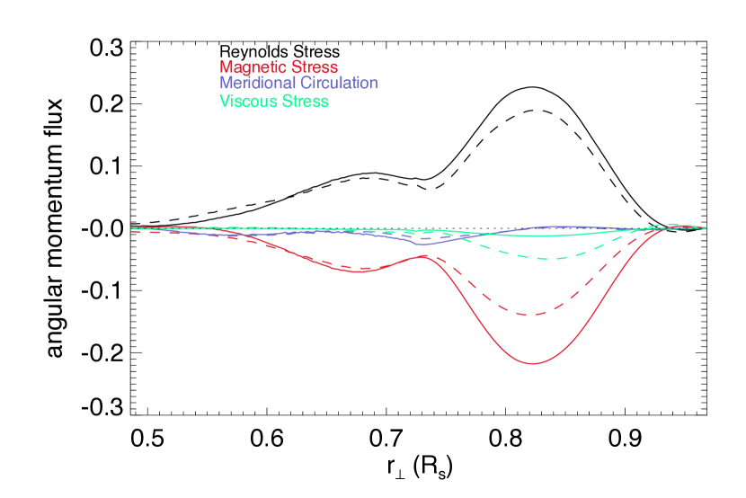
Figure 5: Net angular momentum flux integrated over individual concentric cylinders of radius $r_{\perp}$ centered on the rotation axis produced by the Reynolds stress (black curves), the magnetic stress (red curves), the meridional circulation (blue curves), and the viscous stress (green curves). The solid curves are the results from the current simulation with reduced viscosity and magnetic diffusivity, and the dashed curves give the corresponding results from FF for comparison. Note here for the computation of the viscous flux (the green curves) we have include an estimate of the contribution from the numerical diffusion in addition to that from the explicit viscosity given in equation (19). In the case of the solid green curve, it contains the sole contribution from the numerical diffusion.

Figure 5 shows the net angular momentum flux across individual concentric cylinders $\Sigma(r_{\perp})$ of radius $r_{\perp}$ centered on the rotation axis produced by the Reynolds stress (black curves): $\int_{\Sigma(r_{\perp})}{\bf F}_{\rm RS}\cdot{\hat{\bf r}}_{\perp}d\Sigma$, the magnetic stress (red curves): $\int_{\Sigma(r_{\perp})}{\bf F}_{\rm MS}\cdot{\hat{\bf r}}_{\perp}d\Sigma$, the meridional circulation (blue curves): $\int_{\Sigma(r_{\perp})}{\bf F}_{\rm MC}\cdot{\hat{\bf r}}_{\perp}d\Sigma$, and the viscous stress (green curves): $\int_{\Sigma(r_{\perp})}{\bf F}_{\rm VS}\cdot{\hat{\bf r}}_{\perp}d\Sigma$. The solid curves are the results from the current simulation with reduced viscosity and magnetic diffusivity, and the dashed curves give the corresponding results from FF for comparison. Note here for the green curves showing the viscous flux, we have included in the computation of ${\bf F}_{\rm VS}$ an estimate of the contribution due to the numerical diffusion in addition to that due to the explicit viscosity given by equation (19). In the case for the solid green curve in Figure 5, it contains the sole contribution from the numerical diffusion. From Figure 5 we see that indeed the meridional circulation contributes very little to the net transport of angular momentum across the cylinders. We see a net outward (positive) transport of angular momentum by the Reynolds stress (black curves) throughout the convection zone (except at the very top), which is the driver and cause of the solar-like (faster equator) differential rotation in the convective dynamo. Similar results are also found in Nelson et al. (2013). In FF we found that the presence of the magnetic fields in the convective dynamo is important for the self-consistent maintenance of the solar-like differential rotation. Without the magnetic fields, in the corresponding hydrodynamic case, the net transport of angular momentum by the Reynolds stress reverses to inward across the cylinders, resulting in an anti-solar (faster pole) rotation profile. (This result of changing to an anti-solar rotation with the removal of the magnetic field does not depend on whether the latitude gradient of entropy is imposed at the bottom of the convection zone.) To get a solar-like differential rotation in the hydrodynamic case, a much higher viscosity (by about 5 times the viscosity used in the convective dynamo case in FF) is needed to suppress the convection and obtain an outward transport of angular momentum by the Reynolds stress. In the present convective dynamo simulation where we have reduced the viscosity and the magnetic diffusivity compared to FF, we find that the transport of angular momentum by the Reynolds stress remains outward and its amplitude is enhanced for most of the convection zone compared to the convective dynamo in FF (compare the black solid and black dashed curves in Figure 5). In turn, the inward angular momentum flux by the magnetic stress is also increased (compare the solid and the dashed red curves in Figure 5) to nearly balance the increased Reynolds stress flux, and the net angular momentum flux by the viscous stress is significantly reduced to a negligible level (compare the solid and dashed green curves) because of the removal of the explicit viscosity. The small amount of the remaining flux due to viscous stress as shown by the solid green curve is computed from the numerical diffusion. Here again we see the dynamical effect of the magnetic fields which takes up an effective role of a viscosity.

To assess the relative importance of the numerical and explicit viscosities on smooth, well resolved flows in the case of FF, we have computed in Figure 6a the radial angular momentum flux density due to the explicit viscosity, evaluated at the equator:

$$F_{\rm VS,r}=-\rho_{0}r\nu\left<S_{r\phi}\right>=-\rho_{0}r^{2}\nu\frac{\partial\Omega}{\partial r}$$ (23)

and the corresponding (time and azimuthally averaged) radial angular momentum flux density $F_{\rm NUM,r}$ due to numerical diffusion produced by the upwinded evaluation of the advection term. We see that the amplitude of $F_{\rm NUM,r}$ is typically smaller than that of $F_{\rm VS,r}$ by more than a factor of 3. This suggests that the effective numerical viscosity acting on the well-resolved, smooth variation of $\Omega$ (Figure 6b) is significantly smaller (by typically a factor of 3) than the explicit viscosity $\nu$ in the FF case. The numerical diffusion changes with the local spatial properties of the flows. For non-monotonic grid-scale fluctuations, the numerical diffusivity dominates. But for well resolved flows such as the smoothly varying $\Omega$, we find that the numerical diffusivity is significantly smaller than the explicit viscosity, and thus removing the explicit viscosity in the current case is making a significant difference for the diffusion on the well resolved scales.

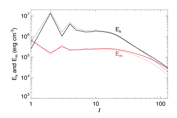
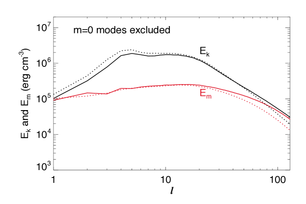
Figure 7: The top panel shows the kinetic ($E_{k}$, black curves) and magnetic ($E_{m}$, red curves) energy spectra as a function of the spherical harmonic degree $l$ at a depth of $0.73R_{\odot}$ near the bottom of the convection zone from our current convective dynamo simulation (solid curves) with reduced viscosity and magnetic diffusivity, and from the convective dynamo of FF (dotted lines). The bottom panel shows the same but with the contribution from the mode with the azimuthal order $m=0$ taken out for each $l$.

The reason for the enhanced outward angular momentum flux by the Reynolds stress (as seen in Fig. 5) in the current case with reduced viscosity and magnetic diffusivity is due to the enhanced magnetic fields, which further suppress convection and makes it more rotationally constrained. The top panel of Figure 7 shows the kinetic (black curves) and magnetic (red curves) energy spectra as a function of the spherical harmonic degree $l$ at a depth of $0.73R_{\odot}$ near the bottom of the convection zone from the present convective dynamo (solid curves) and from the convective dynamo of FF (dotted curves). We show energy spectra up to the highest $l$ (about 128) that is adequately resolved. The bottom panel of Figure 7 shows the same as the top panel but with the contribution from the mode with azimuthal order $m=0$ taken out for each $l$. As a result the large contribution from the differential rotation, which produces the two peaks in the kinetic energy seen at $l=2$ and $l=4$ in the top panel, are removed such that the kinetic energy spectra (in the bottom panel) reflects more closely those for the convective motions. Also the contribution from the (azimuthally averaged) mean magnetic field is removed from the magnetic energy spectra in the bottom panel. Compared to FF, we see that the magnetic energy $E_{m}$ (in both the top and bottom panels) in the present case is enhanced significantly in the small scales and remains about the same in the large scales. The convective kinetic energy on the other hand is reduced in the larger scales, which are the ones more influenced by rotation and contributing to the Reynolds stress transport of angular momentum. These larger scale convective motions become more rotationally constrained due to the reduction in their amplitude and thus producing a greater outward flux of angular momentum by the Reynolds stress. In the smaller scales, the kinetic energy is increased compared to FF, but the magnetic energy is also increased and becomes closer to equipartition with the kinetic energy compared to FF. Thus the magnetic field becomes more dynamically important in the present case than in FF.

We have computed the following energy conversion rates, the buoyancy work $W_{\rm Buoyancy}$, which is the energy source and driving of the convection, and the work done against the Lorentz force $W_{\rm Lorentz}$, which measures the energy conversion from the kinetic energy to the magnetic energy:

$$W_{\rm Buoyancy}=\left<\int_{V}\rho_{0}g_{0}v_{r}\frac{s_{1}}{c_{p}}dV\right>,$$ (24)

$$W_{\rm Lorentz}=-\left<\int_{V}{\bf v}\cdot\left[\frac{1}{4\pi}\left(\nabla\times{\bf B}\right)\times{\bf B}\right]dV\right>,$$ (25)

where the integration is over the entire simulation volume $V$, and “$\left<\right>$” denotes time average. The buoyancy work $W_{\rm Buoyancy}$ is found to be nearly identical for the two cases: being $0.782\pm 0.0023L_{\rm sol}$ for the present simulation and $0.777\pm 0.0024L_{\rm sol}$ for FF, where $L_{\rm sol}$ is the solar luminosity, with the difference being below the 3 sigma level. In other words, the convection is driven (nearly) equally hard in the two convective dynamo simulations. This is probably because both are driven by the same solar radiative diffusive heat flux and we have used the same thermal diffusivity. On the other hand, the work done against the Lorentz force $W_{\rm Lorentz}$ is $0.330\pm 0.0074L_{\rm sol}$ for the present case and $0.256\pm 0.0067L_{\rm sol}$ for FF, i.e. with more kinetic energy converted to the magnetic energy in the present case. Thus, as a result of the reduced viscosity and magnetic diffusion in our present simulation, an increased portion of the (same) buoyancy work is being converted to the magnetic energy, and a decreased portion for work against viscous dissipation. This is another way to see the effective role of the magnetic fields as an enhanced viscosity in suppressing convection.

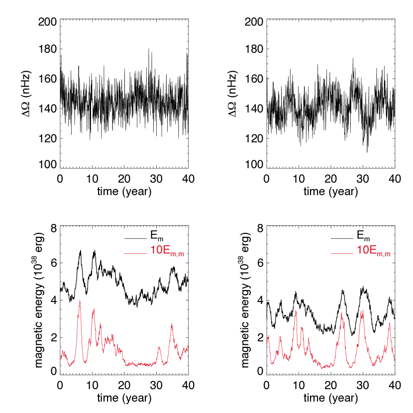
Figure 8: Top panels show the evolution of the differential rotation contrast $\Delta\Omega$ (peak difference in angular rotation rate) and the bottom panels show the corresponding temporal evolution of the total magnetic energy $E_{\rm m}$ (black curve) and ten times the mean magnetic energy $10E_{\rm m,m}$ (red curve), for the present low diffusivity case (left column) and for FF (right column).

Figure 8 shows the temporal evolution of the differential rotation contrast $\Delta\Omega$ (peak difference in angular rotation rate, top panels) and the corresponding temporal evolution of the total and (10 times) the mean magnetic energies (bottom panels), for the present convective dynamo (left column) in comparison to the case of FF (right column). $\Delta\Omega$ on average is slightly bigger, being $144.1\pm 0.2$ nHz in the present case, compared to $142.5\pm 0.3$ nHz for FF. $\Delta\Omega$ shows a temporal variation with an RMS amplitude of about $10$ nHz for both cases, weakly anti-correlated with the total magnetic energy $E_{\rm m}$ as well as the mean magnetic energy $E_{\rm m,m}$. The anti-correlation is weaker in the present case (with a linear correlation coefficient $r=-0.21$ with $E_{m}$ and $r=-0.15$ with $E_{\rm m,m}$ ) compared to FF ($r=-0.44$ with $E_{m}$ and $r=-0.33$ with $E_{\rm m,m}$ ). The magnetic field is playing a complex dual role for the differential rotation. On the one hand it suppresses convection to allow a greater outward transport of the angular momentum by the Reynolds stress to drive a solar-like differential rotation. On the other hand it also damps the differential rotation by balancing the Reynolds stress with the Maxwell stress transport of angular momentum. Such complex dual role may have resulted in a weak anti-correlation.

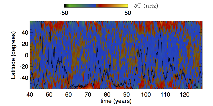
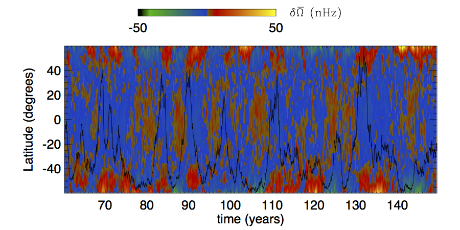
Figure 9: The latitude-time diagram of $\delta\bar{\Omega}(t,\theta)=\bar{\Omega}(t,\theta)-\left<\bar{\Omega}\right>_{t}(\theta)$, where $\bar{\Omega}(t,\theta)$ is the depth averaged angular rotation rate as a function of time and latitude, and $\left<\bar{\Omega}\right>_{t}(\theta)$ is the temporal average of $\bar{\Omega}(t,\theta)$. Thus $\delta\bar{\Omega}(t,\theta)$ shows the deviation from the mean latitudinal differential rotation. The overlaid black curve shows the temporal evolution of the mean magnetic energy. The top panel shows the results for the present low diffusivity case and the bottom panel shows the results from the FF simulation.

Figure 9 shows the latitude-time diagram of the deviation from the (time averaged) mean latitudinal differential rotation, i.e. $\delta\bar{\Omega}(t,\theta)=\bar{\Omega}(t,\theta)-\left<\bar{\Omega}\right>_{t}(\theta)$, where $\bar{\Omega}(t,\theta)$ denotes the depth averaged angular rotation rate as a function of time and latitude, and $\left<\bar{\Omega}\right>_{t}(\theta)$ is the temporal average of $\bar{\Omega}(t,\theta)$. Overlaid on the diagram is the (black) curve showing the temporal variation of the mean magnetic energy $E_{\rm m,m}$. The top panel shows the results for the present low diffusivity case and the bottom panel shows the results from the FF simulation. The main pattern we see is that there is a tendency for negative $\delta\bar{\Omega}$ at the equator and positive $\delta\bar{\Omega}$ in the polar region for magnetic maxima, i.e. the contrast of the (solar-like) latitudinal differential rotation is relatively reduced for magnetic maxima. This anti-correlation is quite weak: we find a linear correlation coefficient between $\delta\bar{\Omega}$ at the equator and $E_{\rm m,m}$ of $r=-0.46$ for the present case and $r=-0.48$ for the FF case.

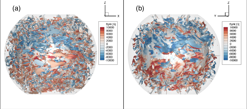
Figure 10: 3D views of iso-surfaces of $v_{a}/v_{\rm rms}=1$ in the convective envelope, where $v_{a}$ is the Alfvén speed and $v_{\rm rms}$ is the RMS convective velocity at that depth. The iso-surfaces outline regions of strong magnetic field concentrations of super-equipartion field strength. (a) results from the current less diffusive convective dynamo simulation and (b) results from the convective dynamo simulation of FF.

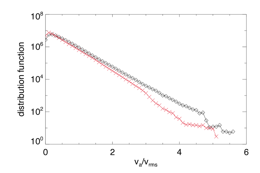
Figure 11: Distribution function of the grid points over the value of $v_{a}/v_{\rm rms}$, where $v_{a}$ is the Alfvén speed and $v_{\rm rms}$ is the RMS convective velocity at that depth. Diamond points are the result for the current less diffusive convective dynamo and the red cross points are the result from FF

Figure 10 shows a 3D view of the magnetic field concentrations in the convective envelope produced by the present convective dynamo simulation (panel (a)), in comparison to that produced by the convective dynamo of FF (panel (b)). The images show iso-surfaces of $v_{a}/v_{\rm rms}=1$ where $v_{a}$ is the Alfvén speed and $v_{\rm rms}$ is the RMS velocity at that depth. The iso-surfaces thus outline regions of strong magnetic field concentrations with super-equipartition field strength. The iso-surfaces are colored with the azimuthal field strength $B_{\phi}$ as indicated by the color table. We see filamentary strong field concentrations of a preferred sign of toroidal field in each hemisphere, antisymmetric for the two hemispheres. Some of these strong filaments emerge towards the top boundary (appearing flattened at the top). Comparing panels (a) and (b) we see that the present, less diffusive convective dynamo shows denser and more smaller scale filaments of strong (super-equipartion) magnetic field concentrations. Figure 11 shows the distribution function of the grid points over the value of $v_{a}/v_{\rm rms}$, where $v_{a}$ is the Alfvén speed and $v_{\rm rms}$ is the RMS convective velocity at that depth, at a magnetic maximum (corresponding to the snapshot shown in Figure 10(a)) for the current less diffusive case (black diamond points) compared to that at a magnetic maximum (corresponding to Figure 10(b)) for the FF case (red cross points). There is clearly more volume occupied by strong super-equipartition fields (with $v_{a}/v_{\rm rms}>1$) in the current less diffusive case, indicating that the magnetic field is more dynamically important.

4 Conclusions

Extending upon the work of FF, we investigate further the dynamical effect of the magnetic fields in the self-consistent maintenance of the solar-like differential rotation by carrying out a simulation of the solar convective dynamo as that described in FF but with further reduced viscosity and magnetic diffusivity. The explicit viscosity and magnetic diffusion in the simulation of FF are removed and only the slope-limited numerical diffusions are present in the current simulation.

As a result, we find that the magnetic energy is enhanced by about 1.5 times, and mainly in the small scales, while the kinetic energy is reduced in the larger scales and increased in the smaller scales, with the total kinetic energy showing a decrease. In the smaller scales, the magnetic energy is increased to approaching equipartition with the kinetic energy. Because of the further suppression of the amplitude of the larger scale convective motions which are most influenced by rotation, they become more rotationally constrained and we found a further increased net outward transport of angular momentum (across the cylinders, away from the rotation axis) by the Reynolds stress, which is in turn balanced by a significantly increased inward transport of the angular momentum by the magnetic stress. The net angular momentum transport by viscous stress is significantly reduced to a negligible level, with the transport by the Reynolds stress nearly entirely balanced by the transport by the magnetic stress. (The net transport by the meridional circulation is also found to be negligible.) The resulting solar-like differential rotation remains essentially the same as that found in FF. The large scale mean field also shows a similar irregular cyclic behavior as that found in FF. We note that our results here and in FF are limited to the case of magnetic Prandtl number of 1. We have also only run the dynamo simulations with a radial magnetic field top boundary condition (which has zero torque from the top boundary to ensure angular momentum conservation of the spherical shell). The result presented in this convective dynamo simulation as an extension of that in FF further demonstrates the dynamical effect of the magnetic field that behaves likes an enhanced viscosity to suppress the convective motions and produce the necessary Reynolds stress transport for maintaining the solar-like differential rotation, as the diffusivities are reduced.

Figure 6: (a) The radial angular momentum flux density $F_{\rm VS,r}$ at the equator due to the explicit viscosity (solid curve), compared to the corresponding (time and azimuthally averaged) radial angular momentum flux density $F_{\rm NUM,r}$ due to numerical diffusion (dash-dotted curve), both computed in the simulation of FF. (b) The time and azimuthally averaged angular frequency $\Omega$ of the differential rotation at the equator (also from the FF case).

References

- Augustson et al. (2015) Augustson, K., Brun, A. S., Miesch, M., & Toomre, J. (2015). Grand Minima and Equatorward Propagation in a Cycling Stellar Convective Dynamo. ApJ, 809, 149. doi:10.1088/0004-637X/809/2/149. arXiv:1410.6547.
- Brun et al. (2004) Brun, A. S., Miesch, M. S., & Toomre, J. (2004). Global-scale turbulent convection and magnetic dynamo action in the solar envelope. ApJ, 614, 1073--1098. URL: http://www.journals.uchicago.edu/doi/abs/10.1086/423835. doi:10.1086/423835. arXiv:http://www.journals.uchicago.edu/doi/pdf/10.1086/423835.
- Christensen-Dalsgaard et al. (1996) Christensen-Dalsgaard, J., Dappen, W., Ajukov, S. V., Anderson, E. R., Antia, H. M., Basu, S., Baturin, V. A., Berthomieu, G., Chaboyer, B., Chitre, S. M., Cox, A. N., Demarque, P., Donatowicz, J., Dziembowski, W. A., Gabriel, M., Gough, D. O., Guenther, D. B., Guzik, J. A., Harvey, J. W., Hill, F., Houdek, G., Iglesias, C. A., Kosovichev, A. G., Leibacher, J. W., Morel, P., Proffitt, C. R., Provost, J., Reiter, J., Rhodes, E. J., Jr., Rogers, F. J., Roxburgh, I. W., Thompson, M. J., & Ulrich, R. K. (1996). The Current State of Solar Modeling. Science, 272, 1286--1292. doi:10.1126/science.272.5266.1286.
- Fan & Fang (2014) Fan, Y., & Fang, F. (2014). A Simulation of Convective Dynamo in the Solar Convective Envelope: Maintenance of the Solar-like Differential Rotation and Emerging Flux. ApJ, 789, 35. doi:10.1088/0004-637X/789/1/35. arXiv:1405.3926.
- Fan et al. (2013) Fan, Y., Featherstone, N., & Fang, F. (2013). Three-Dimensional MHD Simulations of Emerging Active Region Flux in a Turbulent Rotating Solar Convective Envelope: the Numerical Model and Initial Results. ArXiv e-prints, . arXiv:1305.6370.
- Gastine et al. (2013) Gastine, T., Wicht, J., & Aurnou, J. M. (2013). Zonal flow regimes in rotating anelastic spherical shells: An application to giant planets. Icar, 225, 156--172. doi:10.1016/j.icarus.2013.02.031. arXiv:1211.3246.
- Ghizaru et al. (2010) Ghizaru, M., Charbonneau, P., & Smolarkiewicz, P. K. (2010). Magnetic Cycles in Global Large-eddy Simulations of Solar Convection. ApJL, 715, L133--L137. doi:10.1088/2041-8205/715/2/L133.
- Guerrero et al. (2013) Guerrero, G., Smolarkiewicz, P. K., Kosovichev, A. G., & Mansour, N. N. (2013). Differential Rotation in Solar-like Stars from Global Simulations. ApJ, 779, 176. doi:10.1088/0004-637X/779/2/176. arXiv:1310.8178.
- Hotta et al. (2015) Hotta, H., Rempel, M., & Yokoyama, T. (2015). Construction of large-scale magnetic field at high Reynolds numbers. Science, submitted.
- Käpylä et al. (2012) Käpylä, P. J., Mantere, M. J., & Brandenburg, A. (2012). Cyclic Magnetic Activity due to Turbulent Convection in Spherical Wedge Geometry. ApJL, 755, L22. doi:10.1088/2041-8205/755/1/L22. arXiv:1205.4719.
- Karak et al. (2015) Karak, B. B., Käpylä, P. J., Käpylä, M. J., Brandenburg, A., Olspert, N., & Pelt, J. (2015). Magnetically controlled stellar differential rotation near the transition from solar to anti-solar profiles. A&A, 576, A26. doi:10.1051/0004-6361/201424521. arXiv:1407.0984.
- Mabuchi et al. (2015) Mabuchi, J., Masada, Y., & Kageyama, A. (2015). Differential Rotation in Magnetized and Non-magnetized Stars. ApJ, 806, 10. doi:10.1088/0004-637X/806/1/10. arXiv:1504.01129.
- Matt et al. (2011) Matt, S. P., Do Cao, O., Brown, B. P., & Brun, A. S. (2011). Convection and differential rotation properties of G and K stars computed with the ASH code. Astronomische Nachrichten, 332, 897. doi:10.1002/asna.201111624. arXiv:1111.5585.
- Miesch (2005) Miesch, M. S. (2005). Large-Scale Dynamics of the Convection Zone and Tachocline. Living Reviews in Solar Physics, 2, 1.
- Miesch et al. (2006) Miesch, M. S., Brun, A. S., & Toomre, J. (2006). Solar Differential Rotation Influenced by Latitudinal Entropy Variations in the Tachocline. ApJ, 641, 618--625. doi:10.1086/499621.
- Nelson et al. (2013) Nelson, N. J., Brown, B. P., Brun, A. S., Miesch, M. S., & Toomre, J. (2013). Magnetic Wreaths and Cycles in Convective Dynamos. ApJ, 762, 73. doi:10.1088/0004-637X/762/2/73. arXiv:1211.3129.
- Racine et al. (2011) Racine, É., Charbonneau, P., Ghizaru, M., Bouchat, A., & Smolarkiewicz, P. K. (2011). On the Mode of Dynamo Action in a Global Large-eddy Simulation of Solar Convection. ApJ, 735, 46. doi:10.1088/0004-637X/735/1/46.
- Rempel (2005) Rempel, M. (2005). Solar differential rotation and meridional flow: The role of a subadiabatic tachocline for the Taylor-Proudman balance. ApJ, 622, 1320--1332.
- Simitev et al. (2015) Simitev, R. D., Kosovichev, A. G., & Busse, F. H. (2015). Dynamo Effects Near the Transition from Solar to Anti-Solar Differential Rotation. ApJ, 810, 80. doi:10.1088/0004-637X/810/1/80. arXiv:1504.07835.
- Thompson et al. (2003) Thompson, M. J., Christensen-Dalsgaard, J., Miesch, M. S., & Toomre, J. (2003). The Internal Rotation of the Sun. ARA&A, 41, 599--643.