A Computational Investigation of the Finite-Time Blow-Up of the 3D Incompressible Euler Equations Based on the Voigt Regularization

Abstract

We report the results of a computational investigation of two blow-up criteria for the 3D incompressible Euler equations. One criterion was proven in a previous work, and a related criterion is proved here. These criteria are based on an inviscid regularization of the Euler equations known as the 3D Euler-Voigt equations, which are known to be globally well-posed. Moreover, simulations of the 3D Euler-Voigt equations also require less resolution than simulations of the 3D Euler equations for fixed values of the regularization parameter $\alpha>0$. Therefore, the new blow-up criteria allow one to gain information about possible singularity formation in the 3D Euler equations indirectly; namely, by simulating the better-behaved 3D Euler-Voigt equations. The new criteria are only known to be sufficient for blow-up. Therefore, to test the robustness of the inviscid-regularization approach, we also investigate analogous criteria for blow-up of the 1D Burgers equation, where blow-up is well-known to occur.

I Introduction

The 3D Euler equations for incompressible inviscid fluid flow are a source of much mathematical and scientific interest. In particular, these equations exhibit many of the same difficulties as the 3D Navier-Stokes equations in the case of large Reynolds numbers. The question of whether these equations develop a finite-time singularity remains an extremely challenging open problem.

A blow-up criterion for the 3D Euler equations for ideal incompressible flow was reported in Larios_Titi_2009 . This criterion is of a different character than, e.g., the well-known Beale-Kato-Majda criterion Beale_Kato_Majda_1984 . Traditional computational searches for blow-up seek to identify singularities by analyzing the vorticity coming from the 3D Euler equations themselves, which are not known to be globally well-posed, and moreover, are extremely difficult to simulate accurately. In contrast, the blow-up criterion in Larios_Titi_2009 only relies on analyzing the vorticity of the 3D Euler-Voigt equations, which are globally well-posed and can be less computationally intensive to simulate accurately.

An important aspect of the Euler-Voigt model, when used as a regularization for the Euler equations, is that the regularization is inviscid in the sense that it does not add artificial viscosity. Hence, we refer to the Voigt-regularization as an inviscid regularization. Moreover, the Voigt-regularization can be used to stabilize simulations of the Euler equations by a method different from adding artificial viscosity, as is done, e.g., in LES (Large-Eddy Simulation) models (see, e.g., Berselli_Iliescu_Layton_2006_book , and the references therein). Inviscid regularization is distinct from regularizations that use artificial viscosity: while artificial viscosity removes energy from the system, the Euler-Voigt equations conserve a modified energy for all time (see (I.2) below). We use this conservation as one test of the validity of our simulations. Moreover, the blow-up criterion we test is derived from (I.2) and the short-time energy conservation of the 3D Euler equations.

In this article, we describe the first computational search for blow-up of the 3D Euler equations based on a Voigt-type blow-up criterion. We also provide a new blow-up criterion that is similar in character to the criterion in Larios_Titi_2009 , but that has several advantages over it. One interesting result of the present work is that extrapolation to $\alpha=0$ suggests the development of a singularity in the 3D Euler equations. The blow-up time $T_{*}$ coincides approximately with the prediction $T_{*}\approx 4.4\pm 0.2$ in Brachet_Meiron_Orszag_Nickel_Morf_Frisch_1983_JFM (see also Bustamante_Brachet_2012 ). However, the purpose of this work is chiefly to motivate the fluid mechanics computational community toward further investigation of this type of criterion, rather than to make a definite claim about blow-up. Because this is a new approach to studying blow-up, we show how the method provides evidence for blow-up in a case where blow-up is well understood; namely, in the inviscid Burgers equation. For additional corroboration of the method, we also show that blow-up is not detected in the viscous Burgers equation, where it is known that blow-up does not occur.

The Euler-Voigt equations were proposed as an inviscid regularization of the Euler equations in Cao_Lunasin_Titi_2006 , where they were first studied. Their viscous counterpart, called the Navier-Stokes-Voigt equations, were studied much earlier in Oskolkov_1973 ; Oskolkov_1982 . The Euler-Voigt equations are given by

$$-\alpha^{2}\partial_{t}\nabla^{2}\mathbf{u}+\partial_{t}\mathbf{u}+(\mathbf{u}\cdot\nabla)\mathbf{u}+\nabla p =0,$$ (I.1a)

$$\nabla\cdot\mathbf{u} =0,$$ (I.1b)

$$\mathbf{u}(\mathbf{x},0) =\mathbf{u}_{0}(\mathbf{x}).$$ (I.1c)

Here $\alpha>0$ is a regularization parameter having units of length. Note that the usual incompressible Euler equations are formally obtained by setting $\alpha=0$. The unknowns are the fluid velocity field $\mathbf{u}(\mathbf{x},t)=(u_{1},u_{2},u_{3})$, and the fluid pressure $p(\mathbf{x},t)$, where $\mathbf{x}=(x_{1},x_{2},x_{3})$, and $t\geq 0$. In the present work, we consider only the case of periodic boundary conditions. (Periodic boundary conditions are often used in computational studies; the review Gibbon_2008 cites more than twenty such studies.) Without loss of generality, we also assume that $\int_{\Omega}\mathbf{u}_{0}(\mathbf{x})\,d\mathbf{x}=0$, which with (I.1a) and (I.1b) implies $\int_{\Omega}\mathbf{u}(\mathbf{x},t)\,d\mathbf{x}=0$ for all $t$. We denote by $\mathbf{u}^{\alpha}$ the solution to (I.1), and by $\mathbf{u}$ a solution to the Euler equations, both starting from the same initial condition $\mathbf{u}_{0}$. In addition, we denote the corresponding vorticities $\boldsymbol{\omega}:=\nabla\times\mathbf{u}$, and also $\boldsymbol{\omega}^{\alpha}:=\nabla\times\mathbf{u}^{\alpha}$.

System (I.1) was introduced in Cao_Lunasin_Titi_2006 , where existence and uniqueness of solutions was proven for all times $t\in(-\infty,\infty)$. The Euler-Voigt and Navier-Stokes-Voigt equations have been studied analytically and extended in a wide variety of contexts (see, e.g., Bohm_1992 ; Catania_2009 ; Catania_Secchi_2009 ; Cao_Lunasin_Titi_2006 ; Larios_Titi_2009 ; Larios_Lunasin_Titi_2015 ; Ebrahimi_Holst_Lunasin_2012 ; Levant_Ramos_Titi_2009 ; Khouider_Titi_2008 ; Olson_Titi_2007 ; Oskolkov_1973 ; Oskolkov_1982 ; Ramos_Titi_2010 ; Kalantarov_Levant_Titi_2009 ; Kalantarov_Titi_2009 , and the references therein). The first computational study of the Navier-Stokes-Voigt and MHD-Voigt equations was carried out in Kuberry_Larios_Rebholz_Wilson_2012 . A recent computational study DiMolfetta_Krstlulovic_Brachet_2015 studied the energy spectrum and other properties of the Euler-Voigt equations. Energy decay for Navier-Stokes-Voigt was studied in Layton_Rebholz_2013_Voigt .

In Cao_Lunasin_Titi_2006 , an “$\alpha$-energy” equality was proved to hold for solutions of (I.1) for all $t\in\mathbb{R}$, namely,

$$E_{\alpha}(t):=\|\mathbf{u}^{\alpha}(t)\|_{L^{2}}^{2}+\alpha^{2}\|\nabla\mathbf{u}^{\alpha}(t)\|_{L^{2}}^{2}=E_{\alpha}(0).$$ (I.2)

One aim of this paper is to investigate the connection between the Euler equations and Euler-Voigt equations as $\alpha\rightarrow 0$. In Larios_Titi_2009 , it was shown that, for sufficiently smooth initial data, on the time interval $[0,T]$ of existence and uniqueness for strong solutions of the Euler equations, the following estimate holds:

$$\|\mathbf{u}(t)-\mathbf{u}^{\alpha}(t)\|_{L^{2}}^{2}+\alpha^{2}\|\nabla(\mathbf{u}(t)-\mathbf{u}^{\alpha}(t))\|_{L^{2}}^{2}$$ (I.3)

$$\leq C\alpha^{2}(e^{Ct}-1),$$

where the constant $C$ depends on $\|\mathbf{u}\|_{L^{\infty}(0,T;H^{3})}$. In particular, as $\alpha\rightarrow 0$, solutions to (I.1) converge to the solution the Euler equations in the $L^{\infty}([0,T];L^{2})$ norm at a rate no worse than $\mathcal{O}(\alpha)$. Combining this with (I.2) and the equality $\|\mathbf{u}(t)\|_{L^{2}}=\|\mathbf{u}_{0}\|_{L^{2}}$, which holds on $[0,T]$, it was proved in Larios_Titi_2009 , by contradiction, that if

$$\sup_{t\in[0,T^{*}]}\limsup_{\alpha\rightarrow 0^{+}}\,(\alpha\|\nabla\mathbf{u}^{\alpha}(t)\|_{L^{2}})>0,$$ (I.4)

then the 3D Euler equations must develop a singularity at or before time $T^{*}$. We shall show in Section II that if

$$\limsup_{\alpha\rightarrow 0^{+}}\Big{(}\alpha\sup_{t\in[0,T^{*}]}\|\nabla\mathbf{u}^{\alpha}(t)\|_{L^{2}}\Big{)}>0,$$ (I.5)

then again the 3D Euler equations must develop a singularity at or before time $T^{*}$. As noted below, (I.4) implies (I.5), and hence (I.5) is a stronger criterion than (I.4), i.e., singularities indicated by (I.4) will also be indicated by (I.5).

Remark I.1.

Comparison with original criterion. The new blow-up criterion (I.5) is stronger than (I.4), since, for any $u^{\alpha}\in C([0,T],L^{2})\cap L^{1}([0,T],H^{1})$,

$$\sup_{t\in[0,T]}\alpha\|\nabla u^{\alpha}(t)\|_{L^{2}}\geq\alpha\|\nabla u^{\alpha}(t)\|_{L^{2}},$$ (I.6)

for any $t\in[0,T]$, so we may take the $\limsup_{\alpha\to 0^{+}}$ of both sides to obtain

$$\limsup_{\alpha\to 0^{+}}\sup_{t\in[0,T]}\alpha\|\nabla u^{\alpha}(t)\|_{L^{2}}\geq\limsup_{\alpha\to 0^{+}}\alpha\|\nabla u^{\alpha}(t)\|_{L^{2}}.$$ (I.7)

The left-hand side is constant, and the right-hand side depends on t. Thus,

$$\limsup_{\alpha\to 0^{+}}\sup_{t\in[0,T]}\alpha\|\nabla u^{\alpha}(t)\|_{L^{2}}\geq\sup_{t\in[0,T]}\limsup_{\alpha\to 0^{+}}\alpha\|\nabla u^{\alpha}(t)\|_{L^{2}}.$$ (I.8)

Therefore, if the right-hand side is positive, the left-hand side is positive. Hence, (I.4) implies (I.5).

The computational search for blow-up has a rich recent history, see, e.g. Brachet_Meiron_Orszag_Nickel_Morf_Frisch_1983_JFM ; Brachet_Meiron_Orszag_Nickel_Morf_Frisch_1984_JSP ; Bustamante_2011 ; Cichowlas_Brachet_2005 ; Deng_Hou_Yu_2005 ; Grafke_Grauer_2013_Lagrangian_no_blow_up ; Grafke_Homann_Dreher_Grauer_2007 ; Hou_2009 ; Hou_Lei_Luo_Wang_Zou_2014_Euler ; Hou_Li_2006_Depletion ; Hou_Li_2008_Blowup ; Hou_Li_2008_Numerical ; Kerr_1993 ; Kerr_2013_Euler_Blowup ; Luo_Hou_2013_Potentially_Singular ; Luo_Hou_2014_Euler_BlowUp ; Pouquet_Brachet_Mininni_2010_TG_MHD ; Siegel_Caflisch_2009 and the references therein. Since it is unknown whether the 3D Euler equations become singular in a finite interval of time, several criteria for the blow-up of solutions have arisen in the literature, e.g., Beale_Kato_Majda_1984 ; Cheskidov_Shvydkoy_2014_unified_blow_up ; Cheskidov_Shvydkoy_2014_unified_blow_up ; Constantin_Fefferman_1993 ; Constantin_Fefferman_Majda_1996 ; Ferrari_1993 ; Gibbon_Titi_2013_Blowup ; Kozono_Ogawa_Taniuchi_2002 ; Ponce_1985 . Perhaps the most celebrated is the Beale-Kato-Majda criterion Beale_Kato_Majda_1984 which states that the solution is non-singular on $[0,T]$ if and only if

$$\int_{0}^{T}\|\boldsymbol{\omega}(t)\|_{L^{\infty}}\,dt<\infty.$$ (I.9)

Hence, in many computational searches for blow-up of solutions of the Euler equations (see, e.g., Deng_Hou_Yu_2005 ; Hou_2009 ; Hou_Li_2008_Blowup ; Hou_Li_2008_Numerical ; Kerr_1993 ; Kerr_2013_Euler_Blowup , and references therein), $\|\boldsymbol{\omega}(t)\|_{L^{\infty}}$ is the main quantity of interest. Thanks to the identity $\|\nabla\mathbf{v}\|_{L^{2}}=\|\nabla\times\mathbf{v}\|_{L^{2}}$, holding for all smooth divergence-free functions $\mathbf{v}$, one can view (I.4) and (I.5) as conditions on the vorticity $\boldsymbol{\omega}^{\alpha}$ of the Euler-Voigt equations. In Fig. I.1, we plot the time evolution of the $L^{2}$ energy spectrum, which is captured within an accuracy of $10^{-12}$.

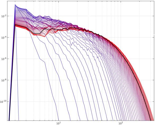
Figure I.1: The $L^{2}$ spectrum vs. wave number the solution of the Euler-Voigt equations with $\alpha=12/1024$ at times $t=0.0,0.1,\ldots,4.9,5.0$. At $t=0.0$, the spectrum is blue. It becomes increasing red as time evolves. The black spectrum corresponds to time $4.2$, where the smallest slope is observed in Fig. IV.1. Resolution: $N^{3}=1024^{3}$.

Remark I.2.

We emphasize that quantity (I.9) is computed from solutions of the 3D Euler equations, which are not known to be globally well-posed. In contrast, the quantity $\|\nabla\mathbf{u}^{\alpha}\|_{L^{2}}$ in (I.4) and (I.5) is computed from solutions to (I.1), which is known to be well-posed globally in time. This gives a mathematical foundation for reliably computing $\|\nabla\mathbf{u}^{\alpha}\|_{L^{2}}$. Moreover, due to (I.2), the growth of the gradient—and hence the development of small length scales—is limited. This is important in numerical simulations, where one has only finite resolution. In contrast, the 3D Euler equations are not known to possess such a quality.

In Section II, we improve criterion (I.4) to criterion (I.5). Numerical methods are described in Section III. The main work is in Section IV, where we computationally investigate the dependence of $\|\nabla\mathbf{u}^{\alpha}(t)\|_{L^{2}}$ on $\alpha$ and $t$, for some given initial data, as $\alpha\rightarrow 0$. It is unknown whether (I.5) (or (I.4)) is a necessary condition for the blow-up of solutions of the 3D Euler equations. Hence, to further support the notion that blow-up may be indicated by (I.5), we consider the 1D inviscid Burgers equation, which is well-known to have solutions that blow up in finite time. In Section V, we apply a Voigt-type regularization to the 1D Burgers equation (yielding the Benjamin-Bona-Mahoney (BBM) equation (V.1)), and show computationally that the analogues of (I.4) and (I.5) appear to be satisfied when $T^{*}$ approaches the blow-up time of the Burgers equation. Moreover, we show that (I.5) is no longer satisfied after the addition of viscosity, which conforms with the global-well-posedness of the viscous Burgers equation.

II Improved Blow-Up Criterion

In this section, we improve blow-up criterion (I.4) to blow-up criterion (I.5). Both criteria are derived from (I.2) and the short-time energy conservation of the 3D Euler equations; hence, we briefly discuss recent work relating energy conservation to smoothness.

We denote by $L^{p}$ and $H^{s}$ the usual Lebesgue and Sobolev spaces over the periodic domain $\Omega\equiv[0,1]^{3}:=\mathbb{R}^{3}/\mathbb{Z}^{3}$, respectively. It is a classical result (see, e.g., Majda_Bertozzi_2002 ; Marchioro_Pulvirenti_1994 ) that, for initial data $\mathbf{u}_{0}\in H^{3}$ satisfying $\nabla\cdot\mathbf{u}_{0}=0$, a unique strong solution $\mathbf{u}$ of the 3D Euler equations exists and is unique on a maximal time interval that we denote by $[0,T^{*})$. Moreover, one has

$$\|\mathbf{u}(t)\|_{L^{2}}=\|\mathbf{u}_{0}\|_{L^{2}}\text{ on }[0,T^{*}).$$ (II.1)

Equation (II.1) holds under weaker conditions on the smoothness of the solutions of the 3D Euler equations, as it was conjectured by Onsager (see, e.g., Cheskidov_Constantin_Friedlander_Shvydkoy ; Constantin_E_Titi_1994 ; Eyink_1994 ; Eyink_Sreenivasan_2006 ; Onsager_1949 ). However, the existence of such weak solutions for arbitrary admissible initial data is still out of reach. In Bardos_Titi_2010 , it was shown that a certain class of shear flows are weak solutions in $L^{\infty}((0,T);L^{2})$ that conserve energy. Furthermore, families of weak solutions that do not satisfy the regularity assumed in the Onsager conjecture have been constructed that do not satisfy (II.1), see, e.g., Buckmaster_DeLellis_Isett_Szekelyhidi_2015 ; Buckmaster_2015 ; DeLellis_Szekelyhidi_2010_admissibility ; DeLellis_Szekelyhidi_2013 ; DeLellis_Szekelyhidi_2014_Onsager ; Isett_2013_thesis .

The following theorem was proved in Larios_Titi_2009 . It is based on a similar theorem for the surface quasi-geostrophic (SQG) equations in Khouider_Titi_2008 .

Theorem II.1 (Larios_Titi_2009 ).

Assume $\mathbf{u}_{0}\in H^{s}$, for some $s\geq 3$, with $\nabla\cdot\mathbf{u}_{0}=0$. Suppose there exists a $T>0$ such that solutions $\mathbf{u}^{\alpha}$ of (I.1) satisfy (I.4). Then the 3D Euler equations, with initial data $\mathbf{u}_{0}$, must develop a singularity within the interval $[0,T]$.

A technical difficulty arises in computational tests of Theorem II.1. Mathematically, one may imagine fixing a $t>0$ and computing

$$\limsup_{\alpha\rightarrow 0^{+}}\left(\alpha\|\nabla\mathbf{u}^{\alpha}(t)\|_{L^{2}}\right).$$ (II.2)

However, computationally, it is more natural to first fix $\alpha>0$ as a parameter, and then to compute $\mathbf{u}^{\alpha}(t)$ as $t$ increases up to a time $T$ (e.g., by a standard time-stepping method). Therefore, to construct curves of $\alpha\|\nabla\mathbf{u}^{\alpha}(t)\|_{L^{2}}$ vs. $\alpha$ for each fixed $t$, one must jump from solution to solution as $\alpha$ varies. This gives rise to some of the technical issues discussed above. However, suppose for a moment that one is allowed to commute the two limiting operations in (I.4). One would then obtain criterion (I.5). The quantity in (I.5) is arguably easier to track, as discussed above. It is the purpose of this section to show rigorously that (I.5) implies that the 3D Euler equations develop a singularity within the interval $[0,T]$.

Let $T>0$ be given. Assume that a given solution to the Euler equations is smooth on $[0,T]$, so that in particular, (II.1) holds. We emphasize that (II.1) depends on the regularity of the 3D Euler equations, and if a finite-time singularity develops, (II.1) might not hold.

Theorem II.2.

Let $\mathbf{u}_{0}\in H^{s}$, $s\geq 3$, with $\nabla\cdot\mathbf{u}_{0}=0$, and let $\mathbf{u}^{\alpha}$ be the corresponding unique solution of (I.1). Suppose that (I.4) holds for some $T>0$. Then the Euler equations must develop a singularity within the interval $[0,T]$.

Proof.

We prove the contrapositive. Assume that $\mathbf{u}$ is a solution of the 3D Euler equations, with initial data $\mathbf{u}_{0}\in H^{s}$, $s\geq 3$, that remains smooth on the interval $[0,T]$. In particular, the smoothness implies that (II.1) holds. From (I.3), for any $t\in[0,T]$, it follows that

$$\|\mathbf{u}^{\alpha}(t)\|_{L^{2}} \geq\|\mathbf{u}(t)\|_{L^{2}}-C\alpha(e^{Ct}-1)^{1/2}$$ (II.3)

$$\geq\|\mathbf{u}(t)\|_{L^{2}}-C\alpha(e^{CT}-1)^{1/2}$$ (II.4)

$$=\|\mathbf{u}_{0}\|_{L^{2}}-C\alpha(e^{CT}-1)^{1/2}.$$

Here, we have used (II.1). Let $\alpha>0$ be sufficiently small so that the right-hand side is positive (e.g., choose, $\alpha<\|\mathbf{u}_{0}\|_{L^{2}}/(C(e^{CT}-1)^{1/2})$. Squaring, we obtain,

$$\|\mathbf{u}^{\alpha}(t)\|_{L^{2}}^{2} \geq\|\mathbf{u}_{0}\|_{L^{2}}^{2}-2C\alpha\|\mathbf{u}_{0}\|_{L^{2}}(e^{CT}-1)^{1/2}$$ (II.5)

$$\qquad+C^{2}\alpha^{2}(e^{CT}-1).$$

Combining (II.5) and (I.2), we discover

$$\alpha^{2}\|\nabla\mathbf{u}^{\alpha}(t)\|_{L^{2}}^{2} \leq\alpha^{2}\|\nabla\mathbf{u}_{0}\|_{L^{2}}^{2}+2C\alpha\|\mathbf{u}_{0}\|_{L^{2}}(e^{CT}-1)^{1/2}$$

$$\qquad-C^{2}\alpha^{2}(e^{CT}-1).$$

Thus, $\limsup_{\alpha\rightarrow 0^{+}}\sup_{t\in[0,T]}\alpha^{2}\|\nabla\mathbf{u}^{\alpha}(t)\|_{L^{2}}^{2}=0,$ which contradicts assumption (I.4), and therefore the solution $\mathbf{u}$ of the Euler equations must become singular within the interval $[0,T]$. ∎

III Numerical Methods

All simulations were carried out using a pseudospectral method on the periodic unit cube; namely, with derivatives computed in Fourier space, and products computed in physical space with the $2/3$’s dealiasing rule applied. Time stepping for the inviscid equations was done using a fully-explicit fourth-order Runge-Kutta-4 scheme complying with the advective CFL condition. (For the viscous Burgers equation, an integrating-factor method adapted to Runge-Kutta-4 was used to avoid the viscous CFL restriction.) The pressure was computed explicitly by the standard Chorin-Temam projection method Chorin_1968 ; Temam_1969_projection . For the Euler-Voigt simulations, Taylor-Green initial data was used on the domain $[0,1]^{3}$, namely,

$$\begin{split}u_{1}&=\phantom{-}\sin(2\pi x)\cos(2\pi y)\cos(2\pi z),\\ u_{2}&=-\cos(2\pi x)\sin(2\pi y)\cos(2\pi z),\\ u_{3}&=0.\end{split}$$ (III.1)

This choice of initial data is very commonly used in computational studies of blow-up for the 3D Euler equations. See, e.g., Brachet_Meiron_Orszag_Nickel_Morf_Frisch_1984_JSP ; Brachet_Meiron_Orszag_Nickel_Morf_Frisch_1983_JFM .

It is important for this study that the energy and the enstrophy are properly captured. Therefore, we consider the maximum relative error in the $\alpha-$energy by

$$\varepsilon_{\text{rel}}:=\max_{t\in[0,T]}\left\lvert\frac{E_{\alpha}(t)-E_{\alpha}(0)}{E_{\alpha}(0)}\right\rvert.$$

Due to the Runge-Kutta-4 time stepping, perfect $\alpha-$energy conservation is not expected. However, every Euler-Voigt simulation at resolution $1024^{3}$ and $512^{3}$ reported in this article had $\varepsilon_{\text{rel}}<2.2\times 10^{-11}$ over the time interval of integration. For the inviscid BBM simulations, $\varepsilon_{\text{rel}}<2.4\times 10^{-14}$. For the viscous BBM simulations, $\varepsilon_{\text{rel}}<2.8\times 10^{-13}$ (for the viscous simulations the definition of $E_{\alpha}(t)$ was adapted to include the term $2\nu\int_{0}^{t}\|u_{x}(s)\|_{L^{2}}\,ds$, computed using Runge-Kutta-4 integration). In Fig. III.1, one can see the typical behavior of the terms comprising the $\alpha$-energy $E_{\alpha}(t)$, with a transfer of the energy ($\|\mathbf{u}^{\alpha}\|_{L^{2}}^{2}$) to the scaled enstrophy ($\alpha^{2}\|\nabla\mathbf{u}^{\alpha}\|_{L^{2}}^{2}$).

(a) $\alpha=4/256$

(b) $\alpha=2/256$

(c) $\alpha=1/256$

Figure III.1: Energy and enstrophy (scaled by $\alpha^{2}$) vs. time for the 3D Euler-Voigt equations. (red “$+$”: $\|\mathbf{u}^{\alpha}(t)\|_{L^{2}}^{2}$, blue “*”: $\alpha^{2}\|\nabla\mathbf{u}^{\alpha}(t)\|_{L^{2}}^{2}$, black “$\circ$”: $\|\mathbf{u}^{\alpha}(t)\|_{L^{2}}^{2}+\alpha^{2}\ \nabla\mathbf{u}^{\alpha}(t)\|_{L^{2}}^{2}$.) Resolution: $256^{3}$.

Remark III.1.

We emphasize that, since (I.1) is globally well-posed in time, we are allowed to integrate the equations beyond the point of possible singularity for the 3D Euler equations. That is, if the Euler equations develop a singularity at time $T^{*}$, for given initial data, we may safely integrate (I.1) with the same initial data up to and beyond $T^{*}$. We believe this to be a major distinction of the blow-up criteria (I.4) and (I.5) from other blow-up criteria for the 3D Euler equations, such as (I.9).

IV Singularity Detection

In this section, we computationally investigate the blow-up criterion (I.5). We simulate solutions of (I.1) with initial data (III.1), tracking the quantity

$$\|\nabla\mathbf{u}^{\alpha}(t)\|_{L^{2}}\equiv\|\boldsymbol{\omega}^{\alpha}(t)\|_{L^{2}},$$ (IV.1)

for several values of $t$, as $\alpha\rightarrow 0$, shown in Fig. IV.1 as contours of constant $t$. Let us make the ansatz that

$$\sup_{t\in[0,T^{*}]}\|\nabla\mathbf{u}^{\alpha}(t)\|_{L^{2}}\sim\mathcal{O}(\alpha^{p}),$$ (IV.2)

for $T^{*}>0$ sufficiently large and for some power $p$. If $p\leq-1$, then (I.5) holds, and the Euler equations develop a singularity within the interval $[0,T^{*}]$. The quantity in (IV.2) is shown in Fig. IV.1 as a function of $\alpha$ with various values of $T^{*}$. The slope of the lines corresponding to $T^{*}\approx 4.2$ are strictly less than $-1$ for small $\alpha$, indicating a possible blow-up of the Euler equations near time $T^{*}\approx 4.2$.

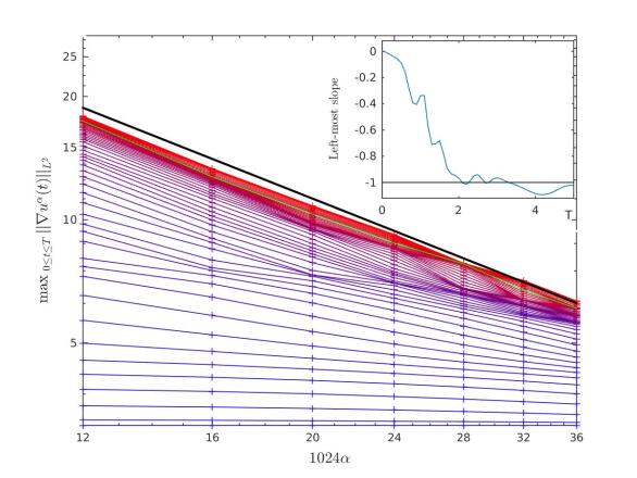
Figure IV.1: Log-log plot of $\max_{t\in[0,T^{*}]}\|\nabla\mathbf{u}^{\alpha}(t)\|_{L^{2}}$ vs. $\alpha$ for the 3D Euler-Voigt equations at $T=0.0,0.1,\ldots,4.9,5.0$, $\alpha=12/1024,\ldots,36/1024$. The thick black line is $C\alpha^{-1}$ vs. $\alpha$. Green curve corresponds to $T=4.2$. Resolution: $N^{3}=1024^{3}$ for $\alpha\leq 24/1024$, $N^{3}=512^{3}$ $\alpha\geq 28/1024$. Inset: Slope between $\alpha=12/1024$ and $\alpha=16/1024$. Minimum value of $-1.0931$ at $T=4.2$.

V Blow-Up for Burgers via the Benjamin-Bona-Mahony Equations

In this section, we consider the 1D Benjamin-Bona-Mahony (BBM) equation for water waves, given by

$$-\alpha^{2}u_{txx}+u_{t}+uu_{x}=0,\qquad u(x,0)=u_{0}(x).$$ (V.1)

This equation was derived in Benjamin_Bona_Mahony_1972 as a model for water waves, where it was shown to be globally well-posed. It can be viewed as a regularization of the inviscid Burgers equation by formally setting $\alpha=0$ in (V.1). Notably, we do not propose here that the solution of (V.1) converges to the unique entropy solution of Burgers equation. We view this equation as a 1D analogue of the Euler-Voigt equations, with a crucial difference being that the pressure and the divergence-free condition are absent. One advantage of considering equation (V.1) is that that solutions to the Burgers equation are known to develop a singularity in finite time; a fact that is unknown for solutions of the 3D Euler equations. By following arguments similar to those in Larios_Titi_2009 , it is straight-forward to show that the analogue of (I.5) implies blow-up for the Burgers equation on $[0,T^{*}]$.

We use the method described in Section IV to try to identify the known singularity in Burgers equation ($u_{t}+uu_{x}=0$). That is, we test the analogue of criterion (I.5) for problem (V.1), as $\alpha\rightarrow 0$. The domain is the periodic interval $[-\pi,\pi]$, and the initial data is $u_{0}(x)=-\sin(x)$. The solution of Burgers equation with this initial data develops a singularity at time $T^{*}=1$.

Fig. V.1 is analogous to Fig. V.2. In Fig. V.1, before the (Burgers) blow-up time $T^{*}=1$, the curves tend to decay faster than $\alpha$ as $\alpha\rightarrow 0$. However, slightly after $T=1.0$, the curves become slightly convex on the log-log plot for small $\alpha$. If this trend continues as $\alpha\rightarrow 0$, the analogue of criterion (I.5) implies Burgers equation develops a singularity at or before time $T^{*}\approx 1.138$. This is already known by other means (e.g., the method of characteristics), but the results here serve to corroborate criterion (I.5) as a test for blow-up.

Finally, we repeat the simulation carried out to generate Fig. V.1, except that we use the viscous BBM equation ($\nu=0.005>0$) instead of equation (V.1). Namely, we consider

$$-\alpha^{2}u_{txx}+u_{t}+uu_{x}=\nu u_{xx}.$$ (V.2)

Due to the well-known fact that the viscous Burgers equation ($u_{t}+uu_{x}=\nu u_{xx}$) does not develop a singularity, we expect that criterion (I.5) will not detect a singularity. Indeed, in Fig. V.2 we see that the curves do not obtain the critical slope value of $p=-1$ as $\alpha\rightarrow 0$, and indeed the lowest value is $\approx-0.235$, far away from the critical value. Thus, in the case of Burgers equation, criterion I.5 detects a singularity in the inviscid case, and does not detect one in the viscous case, exactly as expected.

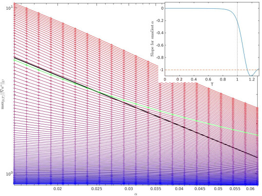
Figure V.1: Log-log plot of $\max_{0\leq t\leq T}\|u^{\alpha}_{x}(t)\|_{L^{2}}$ vs. $\alpha$ or the inviscid ($\nu=0$) BBM equations at various values of $T=0.65,\ldots,1.25$. Green curve corresponds to $T\approx 1.138$. Inset: Slope near smallest $\alpha$-values drops below -1 at $T\approx 1.138$, indicating a blow-up at or before this time. Resolution: $N=8192$.

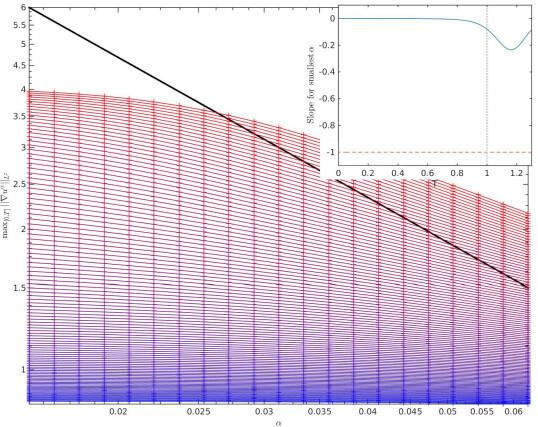
Figure V.2: Log-log plot of $\max_{0\leq t\leq T}\|u^{\alpha}_{x}(t)\|_{L^{2}}$ vs. $\alpha$ for the viscous ($\nu=0.005>0$) BBM equations at various values of T. Same $T$ values as in Fig. V.1. Inset: Slope never drops below -1, meaning no blow-up is detected. Resolution: $N=8192$.

Finally, for two fixed values of $\alpha$, namely $\alpha_{1}=128/8192$ and $\alpha_{2}=138/8192$, we compute the value of the minimum slope as $\nu\rightarrow 0$; that is,

$$S_{\text{min}}(\nu):=\min_{0<t<T}(\|u^{\alpha_{2}}_{x}(t)\|_{L^{2}}-\|u^{\alpha_{1}}_{x}(t)\|_{L^{2}})/(\alpha_{2}-\alpha_{1})$$

as $\nu\rightarrow 0$, where $u^{\alpha_{1}}$ and $u^{\alpha_{1}}$ are solutions to (V.2). This idea was suggested to us by one of the reviewers. It demonstrates the dependence of the blow-up quantity on $\nu$, at least for a given resolution. One can see a smooth transition from right to left as $\nu\rightarrow 0$, crossing the blow-up criterion value of $-1$ roughly at viscosity $\nu_{*}=2.3\times 10^{-4}$. Since Burgers equation is globally well-posed for any $\nu>0$, for $0<\nu\ll 2.3\times 10^{-4}$, the detection yields a false positive for singularity formation here. This underscores the need for higher-resolution studies (which would allow for smaller $\alpha$-values), as well as enhanced extrapolation methods.

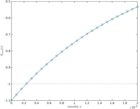
Figure V.3: The quantity $S_{\text{min}}$ vs. $\nu$. This shows the dependence on the minimal slope of the blow-up quantity for values $\alpha_{1}=128/8192$ and $\alpha_{2}=138/8192$. Resolution 8192.

VI Conclusion

The results in Section IV provide computational evidence for the development of a singularity of the 3D Euler equations with Taylor-Green initial data (III.1), near time $T=4.2$. Future studies at smaller $\alpha$-values (and thus higher resolution), combined with state-of-the-art extrapolation methods, may either corroborate or contradict these findings. In any case, the approach presented here represents a new method in the computational search for singularities, and its effectiveness has been demonstrated in the case of Burgers equation.

References

- (1) A. Larios, E.S. Titi, Discrete Contin. Dyn. Syst. Ser. B 14(2/3 #15), 603 (2010)
- (2) J.T. Beale, T. Kato, A.J. Majda, Comm. Math. Phys. 94(1), 61 (1984)
- (3) L.C. Berselli, T. Iliescu, W.J. Layton, Mathematics of large eddy simulation of turbulent flows. Scientific Computation (Springer-Verlag, Berlin, 2006)
- (4) M.E. Brachet, D. Meiron, S. Orszag, B. Nickel, R. Morf, U. Frisch, J. Fluid Mech. 130, 411 (1983)
- (5) M.D. Bustamante, M. Brachet, Phys. Rev. E 86, 066302 (2012).
- (6) Y. Cao, E. Lunasin, E.S. Titi, Commun. Math. Sci. 4(4), 823 (2006)
- (7) A.P. Oskolkov, Zap. Naučn. Sem. Leningrad. Otdel. Mat. Inst. Steklov. (LOMI) 38, 98 (1973).
- (8) A.P. Oskolkov, Zap. Nauchn. Sem. Leningrad. Otdel. Mat. Inst. Steklov. (LOMI) 115, 191 (1982).
- (9) J.D. Gibbon, Phys. D 237(14-17), 1894 (2008).
- (10) M. Böhm, Math. Nachr. 155, 151 (1992).
- (11) D. Catania, Ann. Univ Ferrara 56, 1 (2010).
- (12) D. Catania, P. Secchi, Quad. Sem. Mat. Univ. Brescia (37) (2009)
- (13) A. Larios, E. Lunasin, E.S. Titi, (preprint) arXiv:1010.5024
- (14) M.A. Ebrahimi, M. Holst, E. Lunasin, IMA J. App. Math. pp. 1–26 (2012). Doi:10.1093/imamat/hxr069
- (15) B. Levant, F. Ramos, E.S. Titi, Commun. Math. Sci. 8(1), 277 (2010)
- (16) B. Khouider, E.S. Titi, Comm. Pure Appl. Math. 61(10), 1331 (2008)
- (17) E. Olson, E.S. Titi, Nonlinear Anal. 66(11), 2427 (2007).
- (18) F. Ramos, E.S. Titi, Discrete Contin. Dyn. Syst. 28(1), 375 (2010).
- (19) V.K. Kalantarov, B. Levant, E.S. Titi, J. Nonlinear Sci. 19(2), 133 (2009)
- (20) V.K. Kalantarov, E.S. Titi, Chinese Ann. Math. B 30(6), 697 (2009)
- (21) P. Kuberry, A. Larios, L.G. Rebholz, N.E. Wilson, Comput. Math. Appl. 64(8), 2647 (2012).
- (22) G. Di Molfetta, G. Krstlulovic, M. Brachet, Phys. Rev. E 92, 013020 (2015).
- (23) W.J. Layton, L.G. Rebholz, Int. J. Comput. Fluid Dyn. 27(3), 184 (2013).
- (24) M.E. Brachet, D. Meiron, S. Orszag, B. Nickel, R. Morf, U. Frisch, J. Statist. Phys. 34(5-6), 1049 (1984).
- (25) M.D. Bustamante, Phys. D 240(13), 1092 (2011).
- (26) C. Cichowlas, M.E. Brachet, Fluid Dynam. Res. 36(4-6), 239 (2005).
- (27) J. Deng, T.Y. Hou, X. Yu, Comm. Partial Differential Equations 30(1-3), 225 (2005)
- (28) T. Grafke, R. Grauer, Appl. Math. Lett. 26(4), 500 (2013).
- (29) T. Grafke, H. Homann, J. Dreher, R. Grauer, Phys. D 237(14-17), 1932 (2008).
- (30) T.Y. Hou, Acta Numer. 18, 277 (2009)
- (31) T.Y. Hou, Z. Lei, G. Luo, S. Wang, C. Zou, Arch. Ration. Mech. Anal. 212(2), 683 (2014).
- (32) T.Y. Hou, R. Li, J. Nonlinear Sci. 16(6), 639 (2006).
- (33) T.Y. Hou, R. Li, Phys. D 237(14-17), 1937 (2008).
- (34) T.Y. Hou, R. Li, in Mathematics and computation, a contemporary view, Abel Symp., vol. 3 (Springer, Berlin, 2008), pp. 39–66
- (35) R.M. Kerr, Phys. Fluids A 5(7), 1725 (1993)
- (36) R.M. Kerr, J. Fluid Mech. 729, R2, 13 (2013).
- (37) G. Luo, T.Y. Hou, (2013). arXiv:1310.0497
- (38) G. Luo, T.Y. Hou, Multiscale Model. Simul. 12(4), 1722 (2014).
- (39) A. Pouquet, E. Lee, M.E. Brachet, P.D. Mininni, D. Rosenberg, Geophys. Astrophys. Fluid Dyn. 104(2-3), 115 (2010).
- (40) M. Siegel, R.E. Caflisch, Phys. D 238(23-24), 2368 (2009).
- (41) A. Cheskidov, R. Shvydkoy, J. Math. Fluid Mech. 16(2), 263 (2014).
- (42) P. Constantin, C. Fefferman, Indiana Univ. Math. J. 42(3), 775 (1993).
- (43) P. Constantin, C. Fefferman, A.J. Majda, Comm. Partial Differential Equations 21(3-4), 559 (1996)
- (44) A.B. Ferrari, Comm. Math. Phys. 155(2), 277 (1993)
- (45) J.D. Gibbon, E.S. Titi, J. Nonlinear Sci. 23(6), 993 (2013).
- (46) H. Kozono, T. Ogawa, Y. Taniuchi, Math. Z. 242(2), 251 (2002).
- (47) G. Ponce, Comm. Math. Phys. 98(3), 349 (1985).
- (48) A.J. Majda, A.L. Bertozzi, Vorticity and Incompressible Flow, Cambridge Texts in Applied Mathematics, vol. 27 (Cambridge University Press, Cambridge, 2002)
- (49) C. Marchioro, M. Pulvirenti, Mathematical Theory of Incompressible Nonviscous Fluids, Applied Mathematical Sciences, vol. 96 (Springer-Verlag, New York, 1994)
- (50) A. Cheskidov, P. Constantin, S. Friedlander, R. Shvydkoy, Nonlinearity 21(6), 1233 (2008).
- (51) P. Constantin, W. E, E.S. Titi, Comm. Math. Phys. 165(1), 207 (1994).
- (52) G.L. Eyink, Phys. D 78(3-4), 222 (1994).
- (53) G.L. Eyink, K.R. Sreenivasan, Rev. Modern Phys. 78(1), 87 (2006).
- (54) L. Onsager, Nuovo Cimento (9) 6(Supplemento, 2 (Convegno Internazionale di Meccanica Statistica)), 279 (1949)
- (55) C. Bardos, E.S. Titi, Discrete Contin. Dyn. Syst. Ser. S 3(2), 185 (2010).
- (56) T. Buckmaster, C. De Lellis, P. Isett, L. Székelyhidi, Jr., Ann. of Math. (2) 182(1), 127 (2015).
- (57) T. Buckmaster, Comm. Math. Phys. 333(3), 1175 (2015).
- (58) C. De Lellis, L. Székelyhidi, Jr., Arch. Ration. Mech. Anal. 195(1), 225 (2010).
- (59) C. De Lellis, L. Székelyhidi, Jr., Invent. Math. 193(2), 377 (2013).
- (60) C. De Lellis, L. Székelyhidi, Jr., J. Eur. Math. Soc. (JEMS) 16(7), 1467 (2014).
- (61) P. Isett, ProQuest LLC, Ann Arbor, MI pp. 1–227 (2012). Thesis (Ph.D.)–Princeton University. (arXiv:1211.4065)
- (62) A.J. Chorin, Math. Comp. 22, 745 (1968)
- (63) R. Temam, Arch. Rational Mech. Anal. 32, 135 (1969)
- (64) T.B. Benjamin, J.L. Bona, J.J. Mahony, Philos. Trans. Roy. Soc. London Ser. A 272(1220), 47 (1972)