Resonance model for non-perturbative inputs to gluon distributions in the hadrons

Abstract

We construct non-perturbative inputs for the elastic gluon-hadron scattering amplitudes in the forward kinematic region for both polarized and non-polarized hadrons. We use the optical theorem to relate invariant scattering amplitudes to the gluon distributions in the hadrons. By analyzing the structure of the UV and IR divergences, we can determine theoretical conditions on the non-perturbative inputs, and use these to construct the results in a generalized Basic Factorization framework using a simple Resonance Model. These results can then be related to the $K_{T}$ and Collinear Factorization expressions, and the corresponding constrains can be extracted.

I Introduction

The description of hadronic reactions at high energies requires the use of Quantum Chromodynamics (QCD) in both the perturbative and non-perturbative domains; such calculations are challenging because the non-perturbative characteristics of QCD are difficult to quantify. The standard approach is to use the QCD factorization to divide the problem into perturbative and non-perturbative components, and then use the properties of the perturbative expressions to infer basic features of the non-perturbative piece. We will make use of these properties, together with a simple Resonance Model, to characterize the non-perturbative inputs that enter the hadronic scattering process.

Within the QCD factorization framework, the $2\to n$ hadronic scattering process (for a single parton exchange) is depicted in Fig. 1 where we see the gluon exchange between the hadronic blobs $A_{1,2}$ and the hard scattering process represented by $B$. The remaining partons of hadrons $h_{1,2,}$ which do not participate in the hard interaction are spectators, and they are represented by the outgoing double arrows.

The cross section is related to the square of the factorized amplitudes. We can represent this diagrammatically by combining Fig. 1 together with its mirror image (representing the conjugate amplitude). For the case of Deeply Inelastic Scattering (DIS) where we only have a single hadron, this is depicted in Fig. 2 which shows an incoming hadron ($p$) and photon ($q$) which exchange an intermediate parton ($k$). Here, the lower blob represents the non-perturbative input (Parton Distribution Function) describing the emission/absorption of the exchanged parton $k$ from the initial hadron $p$, and the upper blob corresponds to the interaction between parton $k$ and the incident photon $q$. There is an implied (but not drawn) vertical s-channel cut through this diagram which would represent the DIS on-shell final state of the process. In total, this diagram then represents the DIS hadronic tensor $W^{\mu\mbox{$\nu$}}$ which, when combined with the leptonic tensor $L_{\mu\nu}$, yields the cross section: $d\sigma\sim L_{\mu\nu}W^{\mu\nu}$.

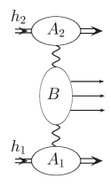
Figure 1: Amplitude for two hadrons ($h_{1}$ and $h_{2}$) with a single parton (gluon) exchange. Blobs $A_{1,2}$ denote the hadrons from which the partons are emitted, and blob B depicts the parton interactions, with the outgoing arrows denoting the produced partons. The outgoing double arrows on blobs $A_{1,2}$ stand for the final state spectators.

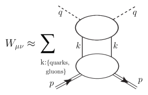
Figure 2: The QCD factorization for the DIS hadronic tensor $W_{\mu\nu}$. The lowest blob includes the non-perturbative input (PDFs), while the upper blob corresponds to DIS of the active parton. If we insert a (vertical) on-shell cut in this diagram (s-cut), it represents a squared amplitude $AA^{*}\sim d\sigma$. Without a cut, it represents an amplitude for a two-parton exchange.

However, without the vertical s-channel cut Fig. 2 can be interpreted as an amplitude $A_{\mu\nu}$ with two partons (each of momentum $k$) being exchanged in the t-channel; essentially, this becomes the elastic Compton scattering process. The optical theorem relates the imaginary part $(\Im)$ of the scattering amplitudes with the cross section, and we can make use of this to relate amplitude $A_{\mu\nu}$ to the hadronic tensor (proportional to the cross section) $W_{\mu\nu}$ as follows:

$$W_{\mu\nu}=\frac{1}{\pi}\ \Im\,A_{\mu\nu}.$$ (1)

Thus we can compute the cross section for the single-exchange DIS process ($d\sigma\sim L_{\mu\nu}W^{\mu\nu}$) using the amplitude for the double-exchange Compton amplitude $A_{\mu\nu}$. In order to avoid misunderstanding, we note that $t$-channel intermediate states in the upper (perturbative) blob can involve unlimited number of partons, even though the blob stands for the $2\to 2$ scattering amplitude. Throughout the paper we will refer to such blobs as non-perturbative inputs regardless of whether they have an s-channel cut or not.

There are a variety of perturbative QCD factorization frameworks in the literature, and each is tailored to a specific purpose. For example, the DGLAP factorizationdglap and its generalizationsegtg1sum describe the case of collinear on-shell partons exchanged in the hadronic tensor $W_{\mu\nu}$. Correspondingly, one therefore needs on-shell non-perturbative inputs (i.e., PDFs) for this calculation; such inputs are the subject of Collinear Factorizationcolfact . In contrast, the BFKL factorizationbfkl operates with essentially off-shell external partons; this precludes a simple matching with the above collinear factorization. Instead, the $K_{T}$-Factorizationktfact (also referred to as High-Energy Factorizationhefact ) can provide a link to the BFKL framework.

These factorizations use different parametrizations for the momentum of the exchanged parton $k$ depending upon which kinematics they wish to emphasize. For example, in Collinear Factorization, we assume the parton $k$ is collinear to the hadron $p$, so we use the single variable $\beta$ to parameterize this relation:

$$k=\beta p.$$ (2)

Thus, $\beta$ is the longitudinal momentum fraction of the parton.

For $K_{T}$-Factorization, the exchanged parton can be off-shell and have a transverse momentum $k_{\perp}$ relative to the hadron momentum $p$, in addition to the longitudinal momentum. We thus use the parametrization:

$$k=\beta p+k_{\perp},$$ (3)

with transverse momentum $k_{\perp}$ parametrizing the two-dimensional transverse space, and as before $\beta$ parametrizes the longitudinal space.

While Eq. (3) is more general than Eq. (2), we can generalize even further using the standard Sudakov representationsud which involves two longitudinal and two transverse parameters:

$$k=-\alpha p^{\prime}+\beta q^{\prime}+k_{\perp}.$$ (4)

Here, the light-cone momenta $p^{\prime},q^{\prime}$ are comprised of the external momenta $p$ and $q$ as follows:

$$p^{\prime}=p-x_{p}q,\quad q^{\prime}=q-x_{q}p,\quad x_{p}=p^{2}/w,\quad x_{q}=q^{2}/w,\quad w=2p^{\prime}q^{\prime}\approx 2pq\ .$$ (5)

They satisfy the inequality $|pq|\gg|p^{2}|,|q^{2}|$ (cf., Fig. 2).

In Ref. egtfact we presented the general factorization form (Basic Factorization) which parametrizes all components of the parton momentum $k$, and this can systematically be related to both $K_{T}$-Factorization and to Collinear Factorization. In the literature, $K_{T}$-Factorization and Collinear Factorization QCD operate with totally different non-perturbative inputs. The Collinear Factorization makes use of the common PDFs which are a function of the parton momentum fraction $x$, while the $K_{T}$-Factorization uses a more generalized non-perturbative object which depends both on $x$ and the $k_{\perp}$ of the parton. While the differences stem from the details of the intended application, analyzing them within the Basic Factorization framework allows us to apply common theoretical constraints which can be derived from the analysis of the infra-red (IR) and ultra-violet (UV) singularities of the factorization convolutions.egtfact Because a physical cross section must be free of any IR and UV cut-offs, we can deduce the properties of the non-perturbative inputs by imposing the condition that these singularities must cancel in the total result.

To further investigate the general case of the Basic Factorization, we will use the Resonance Model as outlined in Ref. egtquark . This model is based on the observation that after a hadron emits a quark or gluon parton, the hadron remnants are unstable and will decay into a number ($n>1$) of resonant states. Ref. egtquark examined the case for quarks, and here we extend this to the case of gluons. We will consider both polarized and unpolarized hadrons, and relate the above general case to both the $K_{T}$ and Collinear Factorizations. Our paper is organized as follows: In Section II we evaluate the elastic gluon-hadron amplitudes for the forward kinematic region in the Born approximation, and then analyze the impact of radiative corrections. We investigate the convergence of the the factorization convolutions to determine the the related constraints on the non-perturbative inputs. We then use those restrictions in Section III within our Resonance Model to construct the non-perturbative inputs for the Basic Factorization, and then derive the corresponding results in the $K_{T}$- and Collinear Factorizations; we consider both polarized and unpolarized gluons. We also compare the results for both the $K_{T}$- and Collinear Factorizations with the commonly used formula from the literature. In Section IV we discuss these results and provide an outlook.

II Elastic gluon-hadron scattering amplitudes with forward kinematics

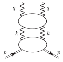
Figure 3: The amplitude factorization of hadron-gluon scattering in the forward kinematic region, with the exchange of intermediate partons (gluons). The upper blob ($H$) depicts $2\to 2$ gluon scattering, and the lower blob ($T$) contains the hadronic target.

In this section we study the elastic gluon-hadron amplitudes in the forward kinematic region for the case of an intermediate gluon. We start with the Basic Factorization framework, and find the conditions for the factorization convolutions to be free of both UV and IR singularities; these restriction will help us model the non-perturbative inputs.

The elastic gluon-hadron scattering amplitude amplitude $A$ receives contributions from both an s-channel and u-channel process; the s-channel is depicted in Fig. 3 and u-channel can be obtained by the replacement $q\to-q$. For this particular set of graphs, the imaginary part ($\Im$) vanishes, so it does not contribute to the gluon distribution.

II.1 Gluon-hadron scattering amplitudes in the Born approximation

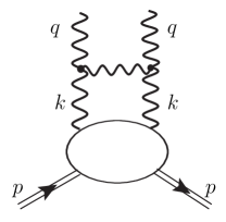
Figure 4: The amplitude factorization of hadron-gluon scattering in the Born approximation, c.f., Fig. 3

In the Basic Factorization framework, the upper blob of Fig. 3 is perturbative while the lower blob includes only non-perturbative contributions. If we work in the Born approximation, the leading contribution for Fig. 3 is a single gluon exchange as shown in Fig. 4. We can use the standard Feynman rules to obtain an analytic expression for the elastic gluon-hadron amplitude $A^{B}$ with non-zero imaginary part $\Im$ in the Born approximation:

$$A^{B}=\frac{4\pi\alpha_{s}N}{(2\pi)^{4}}\int d^{4}k\ l_{\mu}l^{\prime}_{\nu}\,\left[\frac{H_{\mu\nu\lambda\rho}(q,k)}{s_{2}+\imath\epsilon}+\frac{H_{\nu\mu\lambda\rho}(-q,k)}{u_{2}+\imath\epsilon}\right]\frac{1}{k^{2}k^{2}}\,T_{\lambda\rho}(k,p,S),$$ (6)

where $s_{2}=(q+k)^{2}$, $u_{2}=(q-k)^{2}$, $N=3$ is the color factor and $S$ denotes the hadron spin. The term in squared brackets corresponds to the Born amplitude for gluon-gluon scattering, $l_{\mu}(q)$ and $l^{\prime}_{\nu}(q)$ denote the polarization vectors of the external gluons, and the $1/k^{2}$ terms come from the gluon propagators. The contributions from the s-channel and u-channel processes are evident from the $1/(s_{2}+i\epsilon)$ and $1/(u_{2}+i\epsilon)$ terms. The target function $T_{\lambda\rho}$ contains only non-perturbative contributions; it corresponds to the lower blob of Fig. 3 Both $T_{\lambda\rho}$ and the term in the squared brackets are dimensionless. The hard perturbative term $H_{\mu\nu\lambda\rho}$ is given by:

$$H_{\mu\nu\lambda\rho}=\left[(-q-2k)_{\mu}g_{\lambda\sigma}+(2q+k)_{\lambda}g_{\mu\sigma}+(k-q)_{\sigma}g_{\mu\lambda}\right]\left[(q+2k)_{\nu}g_{\rho\sigma}+(-2q-k)_{\rho}g_{\nu\sigma}+(q-k)_{\sigma}g_{\nu\rho}\right]\quad.$$ (7)

$H_{\mu\nu\lambda\rho}$ corresponds to the upper blob of Fig. 3.

For the target function $T_{\lambda\rho}$ we can write the general tensor structure as:

$$T_{\lambda\rho}^{(gen)}=g_{\lambda\rho}A+p_{\lambda}p_{\rho}B+(p_{\lambda}k_{\rho}+k_{\lambda}p_{\rho})C+k_{\lambda}k_{\rho}D\quad.,$$ (8)

where $T_{\lambda\rho}^{(gen)}$ is a function of the relevant momenta $\{p,k\}$ and four arbitrary invariant amplitudes $\{A,B,C,D\}$. If we were to replace the incoming hadron by a bare quark, then the non-perturbative target function $T_{\lambda\rho}$ is replaced by the perturbative quark amplitude $Q_{\lambda\rho}$. This can be decomposed into the unpolarized part $Q_{\lambda\rho}^{U}$ and the spin-dependent part $Q_{\lambda\rho}^{S}$:

$$Q_{\lambda\rho}=Q_{\lambda\rho}^{U}+Q_{\lambda\rho}^{S},$$ (9)

with

$$Q_{\lambda\rho}^{U} = \left(2p_{\mu}p_{\nu}-k_{\mu}p_{\nu}+p_{\mu}k_{\nu}-pk~{}g_{\mu\nu}\right)\left(\frac{-8\pi\alpha_{s}C_{F}}{(p-k)^{2}-m_{q}^{2}+\imath\epsilon}\right),$$ (10)

$$Q_{\lambda\rho}^{S} = \imath m_{q}\epsilon_{\mu\nu\lambda\rho}k_{\lambda}(S_{q})_{\rho}\left(\frac{-8\pi\alpha_{s}C_{F}}{(p-k)^{2}-m_{q}^{2}+\imath\epsilon}\right),$$

where $m_{q}$ is the quark mass, $S_{q}$ is the quark spin and $C_{F}=4/3$.

We will make the assumption that $T_{\lambda\rho}$ keeps the polarization structure of $Q_{\lambda\rho}$ so that:

$$T_{\lambda\rho}=T_{\lambda\rho}^{U}+T_{\lambda\rho}^{S},$$ (11)

with

$$T_{\lambda\rho}^{U} = \left(2p_{\mu}p_{\nu}-k_{\mu}p_{\nu}-p_{\mu}k_{\nu}+pk~{}g_{\mu\nu}\right)\ M_{U}(s_{1},k^{2}),$$ (12)

$$T_{\lambda\rho}^{S} = \imath\,M_{h}\epsilon_{\mu\nu\lambda\rho}k_{\lambda}S_{\rho}\ M_{S}(s_{1},k^{2}),$$

where $s_{1}=(p-k)^{2}$, and $M_{h}$ and $S$ are the hadron mass and spin, respectively. Substituting $T_{\lambda\rho}^{U,S}$ into the elastic gluon-hadron amplitude of Eq. (6), we obtain:

$$A_{U}=\frac{4\pi\alpha_{s}N}{(2\pi)^{4}}\int\frac{d^{4}k}{k^{2}k^{2}}\left[\frac{N_{s}^{(1)}}{s_{2}+\imath\epsilon}+\frac{N_{u}^{(1)}}{u_{2}+\imath\epsilon}\right]M_{U}(s_{1},k^{2}),$$ (13)

$$A_{S}=\frac{4\pi\alpha_{s}N}{(2\pi)^{4}}\int\frac{d^{4}k}{k^{2}k^{2}}\left[\frac{N_{s}^{(2)}}{s_{2}+\imath\epsilon}+\frac{N_{u}^{(2)}}{u_{2}+\imath\epsilon}\right]M_{S}(s_{1},k^{2}),$$ (14)

with

$$N_{s}^{(1)} = 4k^{2}(2m_{h}^{2}+2pk)-16(2(pq)^{2}+2(pq)(pk)-q^{2}(pk))+u_{2}(2M_{h}^{2}-2pk)\ ,$$ (15)

$$N_{s}^{(2)} = \imath M_{h}\epsilon_{\lambda\rho\sigma\tau}S_{\tau}\left[8q_{\rho}\left(l^{\prime}_{\lambda}k_{\sigma}(kl)-l_{\lambda}k_{\sigma}(kl^{\prime})\right)-u_{2}k_{\sigma}l_{\lambda}l^{\prime}_{\rho}\right]\ .$$

For the unpolarized amplitude $A^{U}$, we have summed over the gluon polarizations in the expression for $N_{s}^{(1)}$.

II.2 Analysis of IR and UV singularities

We now examine the IR and UV singularity structure of the $A_{U,S}$ amplitudes. As these quantities are related to physical cross sections, they must ultimately be finite; therefore, the singularities must cancel. In what follows, we will find it convenient to use the Sudakov variables of Eq. (4); specifically, we have:

$$2pk=-\alpha w+\beta x_{p}w,\quad 2qk=\beta w-\alpha xw,\quad k^{2}=-\alpha\beta w+k_{\perp}^{2}\ .$$ (16)

The gluon propagators give rise to the factors $1/k^{2}$, and this will lead to an IR singularity $k^{2}=0$. If we were to introduce an IR cut-off, the result then depends on this unphysical parameter and it must be canceled in the final physical cross section. For the amplitude $A_{U,S}$, which we will relate to a physical cross section using the optical theorem, we are thus unable to introduce any IR cut-off. Therefore, our only option is that the $M_{U,S}$ amplitudes in Eqs. (13,14) must cancel the IR singularities. In order to compensate the $1/(k^{2}k^{2})$ gluon propagators of Eqs. (13,14), in the limit $k^{2}\to 0$ $M_{U,S}$ should obey:

$$M_{U,S}(s_{1},k^{2})\sim\left(k^{2}\right)^{1+\eta}$$ (17)

with $\eta>0$.

We also encounter UV singularities in Eqs. (13,14) at large $|k|$, or equivalently (in terms of the Sudakov variables) at large $|\alpha|$ where the integrands of Eqs. (13,14) behave as:

$$\sim\frac{\alpha^{2}}{\alpha^{3}}\ M_{U,S}\ \equiv\frac{1}{\alpha}\ M_{U,S}\ .$$ (18)

In order to guarantee the amplitudes $A_{U,S}$ are UV finite then $M_{U,S}$ should decrease at large $\alpha$ as:

$$M_{U,S}\sim\alpha^{-\chi},$$ (19)

with $\chi>0$. We note that the restrictions in Eqs. (17,19) apply to the most general polarization structure of $T_{\lambda\rho}$ as given in Eq. (8).

II.3 Gluon-hadron scattering amplitudes beyond the Born approximation

It is relatively easy to extend the above Born result to include radiative corrections. Pictorially, the single gluon exchange of Fig. 4 becomes the generic upper blob of Fig. 3 which now includes the higher-order loop contributions which may be divergent. We now consider the general types of divergences which may enter, and assess whether the radiative corrections will modify the Born restrictions of Eqs. (17,19).

We first consider the case where the upper blob of Fig. 3 acquires additional divergences due to the radiative corrections. As QCD is renormalizable, the UV divergences are absorbed into the redefinition/renormalization of the QCD couplings and masses; there are no complications here. For the IR divergences, these can be regulated with a cut-off such as the parton virtuality $k^{2}$. These procedures will render the amplitude finite.

The upper blob of Fig. 3 represents the generic $2\to 2$ amplitude and can depend only on the total energy $(q+k)^{2}=q^{2}+\omega\beta+k^{2}$ and virtualities $q^{2}$ and $k^{2}$. The only IR divergent terms which can appear at higher order are logarithms such as $\ln(s\beta/k^{2})$; here, $k^{2}$ acts as an IR cut-off, and this logarithmic divergence will not alter the constraint of Eq. (17). Concerning the UV divergences, the upper blob depends on $\alpha$ only through $k^{2}$, so any new $\alpha$-dependent divergences from radiative corrections are also of the logarithmic type; in a similar manner, these divergences will not alter the constraint of Eq. (19).

Let us note that the situation with UV divergences in the conventional factorization approach can be more complex; for example the analysis of UV divergences for $K_{T}$ -factorization is complicated by the existence of rapidity gaps. The essence of the problem is that the perturbative contributions are divided between the upper and lower blob of Fig. 3, and this complicates the cancellation of the UV divergences. The IR divergences are more delicate and must be regulated individually with either a cut-off or a gluon mass regulator; the latter can be easily achieved by keeping the external gluons off-shell so their virtualities act as IR cut-offs for integrations of the loops.

III Modeling the non-perturbative invariant amplitudes $M_{U,S}$

We will now characterize the structure of the non-perturbative inputs to the parton distributions (both the usual and generalized) in the context of the Resonance Model. This was outlined in Ref. egtquark for quark distributions, and we extend it to describe the gluon distributions in the hadrons. We begin by applying this model to the non-perturbative invariant amplitudes $M_{U,S}$ in the Basic Factorization framework, and later we will relate this to the usual $K_{T}$- and Collinear Factorization results.

We review the criteria that invariant amplitudes $M_{U,S}$ should satisfy:

Criterion

(i) $M_{U,S}$ should satisfy the requirements of Eqs. (17,19) so that the physical results are IR and UV finite.

Criterion

(ii) $M_{U,S}$ should have a non-zero imaginary parts in $s_{1}$ to facilitate use of the optical theorem which relates the elastic gluon-hadron amplitudes to gluon distributions in the hadrons.

Criterion

(iii) $M_{U,S}$ should allow for the step-by-step reduction of the Basic Factorization results to those of the $K_{T}$- and Collinear Factorization results.

III.1 Non-perturbative gluon inputs for Basic Factorization

As a first step, we posit that we can decompose the amplitudes $M_{U,S}(s_{1},k^{2})$ into independent functions of the separate momenta $\{s_{1},k^{2}\}$:

$$M_{U}(s_{1},k^{2})=R_{U}\left(k^{2}\right)\ Z_{U}\left(s_{1}\right),\qquad M_{S}(s_{1},k^{2})=R_{S}\left(k^{2}\right)\ Z_{S}\left(s_{1}\right)\ .$$ (20)

In the following we will manipulate $M_{U}$ and $M_{S}$ in parallel, so we drop the subscripts in the following and use: $M(s_{1},k^{2})=R(k^{2})\ Z(s_{1})$. To satisfy the IR constraints of Eq. (17), we find at small $k^{2}$ that $R$ should behave as:

$$R\sim\left(k^{2}\right)^{1+\eta}$$ (21)

Similarly, the UV constraints of Eq. (19) impose the condition:

$$M(s_{1},k^{2})=R(k^{2})\ Z(s_{1})\sim\alpha^{-\chi}$$

at large $|\alpha|$. While the behavior of $R$ at large $|\alpha|$ is ambiguous, it could be that the small-$k^{2}$ behavior at large $|\alpha|$ is again $R\sim(k^{2})^{1+\eta}$. Expressing this in Sudakov variables according to Eq. (16) we have:

$$R\sim\alpha^{1+\eta}.$$ (22)

Since this is the most UV divergent case, we can use this together with Eqs. (19,22) to conclude that $Z$ should behave as:

$$Z\sim\alpha^{-1-\eta-\chi}\ ,$$ (23)

at large $|\alpha|$

We will now construct a $Z$ satisfying Eq. (23) and make use of our Resonance Model. This is based on the idea that after the initial hadron has emitted a parton, the hadron remnant has unbalanced colors and cannot be stable. As we hypothesize that this unstable state will decay into a number of resonances, we then take $Z$ to be a product of Breit-Wigner functions:

$$Z(s_{1})\approx Z_{n}(s_{1})=\prod_{r=1}^{n}\frac{1}{\left(s_{1}-M_{r}^{2}+\imath\Gamma_{r}\right)},$$ (24)

where $n>1$ (since it must decay into multiple resonances). For the sake of simplicity, we consider the minimum allowable value $n=2$ and approximate $Z(s_{1})$ as an interference of two resonances:

$$Z(s_{1})=\frac{1}{\left(\Delta M_{12}^{2}+\imath\Delta\Gamma_{12}\right)}\left[\frac{1}{\left(s_{1}-M_{1}^{2}+\imath\Gamma_{1}\right)}-\frac{1}{\left(s_{1}-M_{2}^{2}+\imath\Gamma_{2}\right)}\right],$$ (25)

with $\Delta M_{12}^{2}=M_{1}^{2}-M_{2}^{2},~{}\Delta\Gamma_{12}=\Gamma_{1}-\Gamma_{2}$. In terms of the Sudakov variables,

$$M(s_{1},k^{2})\equiv M(\alpha,\beta,k^{2})=R(k^{2})\ Z(s_{1})=\frac{R(k^{2})}{C_{Z}}\left[\frac{1}{\left(w\alpha-\mu_{1}^{2}+k^{2}+\imath\Gamma_{1}\right)}-\frac{1}{\left(w\alpha-\mu_{2}^{2}+k^{2}+\imath\Gamma_{2}\right)}\right],$$ (26)

where $C_{Z}=\left(\Delta M_{12}^{2}+\imath\Delta\Gamma_{12}\right)$ and $\mu_{1,2}^{2}=M_{1,2}^{2}-p^{2}$. Applying the optical theorem to Eq. (26) allows us to obtain the non-perturbative contribution $\Psi$ to the gluon distributions in the hadrons:

$$\Psi=-\Im\,T=\widetilde{R}(k^{2})\left[\frac{\Gamma_{1}}{\left(w\alpha+k^{2}-\mu_{1}^{2}\right)^{2}+\Gamma_{1}^{2}}-\frac{\Gamma_{2}}{\left(w\alpha+k^{2}-\mu_{2}^{2}\right)^{2}+\Gamma_{2}^{2}}\right].$$ (27)

Obviously, the expression $\Psi$ is of the Breit-Wigner type because this was the form used in the ansatz for our Resonance Model of Eq. (24).

III.2 Non-perturbative gluon inputs in $K_{T}$- Factorization

The expression in Eq. (26) for the non-perturbative input $M(\alpha,\beta,k^{2})$ is obtained in the Basic Factorization framework. As described in Ref. egtfact ; egtquark , we can relate this to $K_{T}$-Factorization by integrating out the $\alpha$ variable to obtain $M_{KT}\left(\beta,k_{\perp}^{2}\right)$. However, there is a complication because in Fig. 3 both the upper and the lowest blobs depend on $\alpha$, so one cannot integrate $M(\alpha,\beta,k^{2})$ (the lowest blob) over $\alpha$ independently of the upper blob. Therefore, $M_{KT}(\beta,k_{\perp}^{2})$ cannot be derived from $M(\alpha,\beta,k^{2})$ in a straightforward way.

Nevertheless, we can relate the Basic Factorization and the $K_{T}$-Factorization in an approximate manner. We first observe that the upper blob depends on $\alpha$ only through $k^{2}$; if we could limit our integration to the region where the $\alpha$ dependence of the upper blob is negligible, then we can effectively integrate out $\alpha$ to obtain the $K_{T}$-Factorization result; this is our plan. In the integration region when:

$$w|\alpha\beta|\ll k_{\perp}^{2}$$ (28)

the perturbative blobs (the upper blob in Fig. 3) is insensitive to $\alpha$ and the non-perturbative blobs are independent of $\beta$. Because the upper blob depends on $\alpha$ only through $k^{2}$ in the limit of Eq. (28), we can use the approximation $k^{2}=-\omega\alpha\beta-k_{\perp}^{2}\approx-k_{\perp}^{2}$. This makes it possible to integrate $M\left(\alpha,\beta,k^{2}\right)$ independently, and we obtain:

$$M_{KT}(\beta,k_{\perp}^{2})=\int_{-\alpha_{0}}^{\alpha_{0}}d\alpha M(\alpha,\beta,k^{2}),$$ (29)

with

$$\alpha_{0}\ll k_{\perp}^{2}/(w\beta).$$ (30)

In Ref. egtfact we discussed a general structure of non-perturbative inputs in both the Basic and $K_{T}$ -Factorization frameworks, and we estimated $\alpha_{0}$ to be:

$$\alpha_{0}=k_{\perp}^{2}/(w\beta).$$ (31)

Although this estimate adequately describes the main features of the non-perturbative inputs, it is misleading for detailed quantitative analysis. Therefore we need to find an improved estimate for $\alpha_{0}$ that agrees with Eq. (28) and is also independent the variables associated with the perturbative blob such as $\beta$ and $x$. Given that $x<\beta<1$, the requirement in Eq. (28) is satisfied when

$$\alpha_{0}=\xi\>k_{\perp}^{2},$$ (32)

with a positive $\xi$ obeying the inequality $\xi\gg 1/x$. Combining Eqs. (26,29,32) we arrive at the following expression for the non-perturbative input $M_{KT}(\beta,k_{\perp}^{2})$ in $K_{T}$ -Factorization:

$$M_{KT}(\beta,k_{\perp}^{2}) \approx R\left(k_{\perp}^{2}\right)\left[\frac{1}{\xi k_{\perp}^{2}-\mu_{1}^{2}+\imath\Gamma_{1}}+\frac{1}{\xi k_{\perp}^{2}-\mu_{2}^{2}+\imath\Gamma_{2}}+\frac{1}{\xi k_{\perp}^{2}+\mu_{1}^{2}-\imath\Gamma_{1}}+\frac{1}{\xi k_{\perp}^{2}+\mu_{2}^{2}-\imath\Gamma_{2}}\right]$$

$$= R^{\prime}\left(k_{\perp}^{2}\right)\left[\frac{1}{k_{\perp}^{2}-{\mu^{\prime}}_{1}^{2}+\imath\Gamma^{\prime}_{1}}+\frac{1}{k_{\perp}^{2}-{\mu^{\prime}}_{2}^{2}+\imath\Gamma^{\prime}_{2}}+\frac{1}{k_{\perp}^{2}+{\mu^{\prime}}_{1}^{2}-\imath\Gamma^{\prime}_{1}}+\frac{1}{k_{\perp}^{2}+{\mu^{\prime}}_{2}^{2}-\imath\Gamma^{\prime}_{2}}\right],$$

where $R^{\prime}=R/\xi,~{}$, and ${\mu^{\prime}}_{1,2}^{2}=\mu_{1,2}^{2}/\xi,~{}\Gamma^{\prime}_{1,2}=\Gamma_{1,2}/\xi$. We also used $\xi\pm 1\approx\xi$ at large $\xi$. Eq. (III.2) is valid when

$$w\alpha_{0}\gg M_{1,2}^{2},\qquad\Gamma_{1,2}\gg\Delta M^{2},\Delta\Gamma,$$ (34)

that is when $k_{\perp}^{2}$ is away from the resonance region $k_{\perp}^{2}\sim\mu_{1,2}^{2}$. As $k_{\perp}^{2}$ approaches $\mu_{1,2}^{2}$, the corrections to Eq. (III.2) will increase. This means that the relation between the Basic Factorization and the $K_{T}$-Factorization amplitudes of Ref. egtfact is valid with the Resonance Model outside the resonance region; inside the resonance region the corrections can be large, but this can be improved with a redefinition of the parameters $\mu^{\prime}_{1,2}$ and $\Gamma^{\prime}_{1,2}$.

An advantage of Eq. (III.2) is that the resonance form is similar to Eq. (26). In order maintain the validity in the resonance region we choose the following prescription. First, we derive Eq. (III.2) from Eq. (26) in the limit of Eq. (34) and then analytically continue it into the resonance region. Such a strategy is equivalent to independently specifying $M_{KT}$.

Applying the Optical theorem to Eq. (III.2), we obtain the gluon distributions $\Phi$ in the $K_{T}$-Factorization framework, where

$$\Phi=\Phi_{R}+\Phi_{B},$$ (35)

with

$$\Phi_{R}=R^{\prime}\left(k_{\perp}^{2}\right)\left(\frac{\Gamma^{\prime}_{1}}{(k_{\perp}^{2}-{\mu^{\prime}}_{1}^{2})^{2}+{\Gamma^{\prime}}_{1}^{2}}+\frac{\Gamma^{\prime}_{2}}{(k_{\perp}^{2}-{\mu^{\prime}}_{2}^{2})^{2}+{\Gamma^{\prime}}_{2}^{2}}\right)$$ (36)

and

$$\Phi_{B}=-R^{\prime}\left(k_{\perp}^{2}\right)\left(\frac{\Gamma^{\prime}_{1}}{(k_{\perp}^{2}+{\mu^{\prime}}_{1}^{2})^{2}+{\Gamma^{\prime}}_{1}^{2}}+\frac{\Gamma^{\prime}_{2}}{(k_{\perp}^{2}+{\mu^{\prime}}_{2}^{2})^{2}+{\Gamma^{\prime}}_{2}^{2}}\right).$$ (37)

We have divided $\Phi$ into resonance ($\Phi_{R}$) and background ($\Phi_{B}$) contributions which are Breit-Wigner forms. The signs of ${\mu^{\prime}}_{1}^{2}$ and ${\mu^{\prime}}_{2}^{2}$ cannot be fixed a priori, but $\Phi_{R}\to\Phi_{B}$ when ${\mu^{\prime}}_{1,2}^{2}\to-{\mu^{\prime}}_{1,2}^{2}$, so we can take ${\mu^{\prime}}_{1,2}^{2}$ positive without loss of generality. We recall that $k_{\perp}^{2}>0$, so $\Phi_{R}$ is within the resonant region $k_{\perp}^{2}\sim\mu_{1,2}^{2}$, while $\Phi_{B}$ is outside that region. Therefore, the non-perturbative input $\Phi$ in the $K_{T}$ -Factorization is represented by its resonance part $\Phi_{R}$ and the background contribution $\Phi_{B}$. Despite the overall minus sign in Eq. (37), it turns out that the background contribution is positive because the main contribution to the integral of $\Phi_{B}$ over $k_{\perp}^{2}$ comes from the lower limit.

III.3 Non-perturbative gluon inputs in Collinear Factorization

The relation from the non-perturbative input $\Phi(k_{\perp}^{2})$ in $K_{T}$-Factorization to the input $\varphi$ in Collinear Factorization can be obtained by integrating $\Phi$ over $k_{\perp}$. This approximate relation is:

$$\varphi({\mu^{\prime}}_{1}^{2},{\mu^{\prime}}_{2}^{2})\approx\left[R^{\prime}\left({\mu^{\prime}}_{1}^{2}\right)+R^{\prime}\left({\mu^{\prime}}_{2}^{2}\right)\right]-\int_{0}^{w}dk_{\perp}^{2}\Phi_{B}\left(k_{\perp}^{2}\right).$$ (38)

Here, the expression in the squared brackets corresponds to the integration of $\Phi_{R}$, while integration of $\Phi_{B}$ is the explicit integral.

We recall that the non-perturbative inputs $\varphi({\mu^{\prime}}_{1}^{2},{\mu^{\prime}}_{2}^{2})$ differ significantly from the integrated distributions $\phi(\beta,\mu_{col}^{2})$ conventionally used in the Collinear Factorization. These differences include the following important points:

(i)

The non-perturbative inputs $\varphi({\mu^{\prime}}_{1}^{2},{\mu^{\prime}}_{2}^{2})$ do not depend on $\beta$, while the conventional integrated parton distribution $\phi(\beta,\mu_{col}^{2})$ explicitly does depend on this variable.

(ii)

$\varphi({\mu^{\prime}}_{1}^{2},{\mu^{\prime}}_{2}^{2})$ are altogether non-perturbative while $\phi(\beta,\mu_{col}^{2})$ includes both perturbative and non-perturbative contributions.

(iii)

The factorization scale $\mu_{col}$ is arbitrary and usually is chosen in the perturbative domain ($\mu\sim 1$ GeV) while the non-perturbative scales ${\mu^{\prime}}_{1,2}^{2}$ are associated with the maximum of $\Phi(k_{\perp}^{2})$; hence, they cannot be chosen arbitrary and must either be in the non-perturbative or perturbative domain.

III.4 Comparisons with the $K_{T}$ and collinear factorization frameworks

As a final step, we will make a qualitative comparison of $\varphi$ with the standard DGLAP parton distribution. In Eq. (38), $\phi$ does not depend on the longitudinal variable $\beta$. This is in contrast to the parton distributions in the Collinear Factorization framework which explicitly depend on $\beta$, and this can be parametrized as:fits

$$\phi(\beta,\mu^{2})=N\,\beta^{-a}\ (1-\beta)^{b}\,(1+c\beta^{d})\quad,$$ (39)

where $N$ is a normalization, and the phenomenological parameters $a,b,c,d>0$ are fit to experimental data at a specific factorization scale $\mu$. As was demonstrated in Ref. egtg1sum , the $\beta^{-a}$ term of Eq. (39) resums the leading logarithmic contributions; it should be removed when the resummation is included explicitly. Similarly, it is suggested (though not proven) that $(1-\beta)^{b}$ resums the $ln^{n}(1-x)$ terms; again, it should be removed when the resummation is included explicitly. The $(1+c\beta^{d})$ terms resum the residual contributions, and can be removed when the above two resummations are performed. The remaining normalization $N$ then corresponds to the non-perturbative input $\varphi$ obtained in Eq. (38).

While we were able to use the Resonance Model to suggest a form for the $Z$ factor, we do not have an analogous model for R; hence, it is arbitrary up to the restrictions of Eq. (21). In the Basic Factorization framework we have $R\sim\left(k^{2}\right)^{1+\eta}$ at small $k^{2}$, so a possible functional form could be:

$$R=\left(\frac{k^{2}}{k^{2}+M^{2}}\right)^{1+\eta}.$$ (40)

In the $K_{T}$-Factorization framework, $k^{2}$ of Eq. (40) is replaced by $k_{\perp}^{2}$. One possible form for R suggested by Ref. zotov is a Gaussian in $k_{\perp}^{2}$ such as:

$$R=\left[a_{1}\left(k_{\perp}^{2}\right)^{b_{1}}+a_{2}\left(k_{\perp}^{2}\right)^{b_{2}}\right]\exp\left[-\lambda k_{\perp}^{2}\right]\,,$$ (41)

where the factors $a_{1,2}$ and $b_{1,2}$ do not depend on $k_{\perp}^{2}$. Ref. egtfact predicts that $b_{1}>b_{2}\geq 1$. It is evident that both Eq. (40) and Eq. (41) satisfy the restrictions of Eq. (21), so we conclude that some more investigation is required to constrain the form of the $R$ function.

IV Discussion and outlook

In this paper we have constructed the non-perturbative inputs for the elastic gluon-hadron scattering amplitudes in the forward kinematic region for both polarized and non-polarized hadrons. The optical theorem allowed us to relate the invariant amplitudes to the gluon distributions in the hadrons. The conventional approach is purely phenomenological and constructs such inputs by matching with experimental data; in contrast, we use the structure of the IR and UV divergences of the factorization convolutions to determine the general requirements of Eqs. (17,19). Imposing these conditions on the non-perturbative inputs, we constructed the results for the Basic Factorization framework, and then related them systematically to both the $K_{T}$- and Collinear Factorization expressions. In the Basic Factorization framework, the non-perturbative inputs consist of the invariant amplitudes $M_{U,S}$. For simplicity we assumed $M_{U,S}$ had the same polarization structure as for the perturbative case, but this is not obligatory.

We then used the Resonance Model to suggest a form for the $Z$ factors of Eq. (20), and assessed the criteria for which the resonance factors were valid both within and outside of their resonance regions. Starting from the Basic Factorization results, we could then extract the corresponding results for non-perturbative inputs for the $K_{T}$- and Collinear Factorizations. The inputs for $K_{T}$-Factorization of Eqs. (27,III.2) are of the resonance form, and we can then use these to derive the expressions of Eq. (38) for the input $\varphi$ in the Collinear Factorization framework.

V Acknowledgements

We are grateful to A. van Hameren and O.V. Teryaev for useful discussions. We acknowledge the hospitality of CERN, DESY, Fermilab, and UW-INT where a portion of this work was performed. This work was partially supported by the U.S. Department of Energy under grant DE-FG02-13ER41996,

References

- (1) A. Szczurek. Acta Phys.Polon.Supp. 8 (2015) 2, 483
- (2) G. Altarelli and G. Parisi, Nucl. Phys.B126 (1977) 297; V.N. Gribov and L.N. Lipatov, Sov. J. Nucl. Phys. 15 (1972) 438; L.N.Lipatov, Sov. J. Nucl. Phys. 20 (1972) 95; Yu.L. Dokshitzer, Sov. Phys. JETP 46 (1977) 641.
- (3) B.I. Ermolaev, M. Greco, S.I. Troyan. Riv.Nuovo Cim. 33 (2010) 57.
- (4) D. Amati, R. Petronzio, G. Veneziano. Nucl. Phys. B 140 (1978) 54; A.V. Efremov, A.V. Radyushkin. Teor.Mat.Fiz. 42 (1980) 147; Theor.Math.Phys.44 (1980)573; Teor.Mat.Fiz.44 (1980)17; Phys.Lett.B63 (1976) 449; Lett.Nuovo Cim.19 (1977)83; S. Libby, G. Sterman. Phys. Rev. D18 (1978) 3252. S.J. Brodsky and G.P. Lepage. Phys. Lett. B 87 (1979) 359; Phys. Rev. D 22 (1980) 2157; J.C. Collins and D.E. Soper. Nucl. Phys.B 193 (1981) 381; J.C. Collins and D.E. Soper. Nucl. Phys.B 194 (1982) 445; J.C. Collins, D.E. Soper and G. Sterman. Nucl. Phys.B 250 (1985) 199. A.V. Efremov and A.V. Radyushkin. Report JINR E2-80-521; Mod.Phys.Lett. A24 (2009) 2803.
- (5) E.A. Kuraev, L.N. Lipatov and V.S. Fadin, Sov. Phys. JETP 44, 443 (1976); E.A. Kuraev, L.N. Lipatov and V.S. Fadin, Sov. Phys. JETP 45, 199 (1977); I.I. Balitsky and L.N. Lipatov, Sov. J. Nucl. Phys. 28, 822 (1978).
- (6) S. Catani, M. Ciafaloni, F. Hautmann. Phys. Lett. B 242 (1990) 97; Nucl.Phys.B366 (1991) 135.
- (7) J.C. Collins, R.K. Ellis. Nucl.Phys. B360 (1991) 3.
- (8) V.V. Sudakov. Sov. Phys. JETP 3(1956)65.
- (9) B.I. Ermolaev, M. Greco, S.I. Troyan. Eur.Phys.J. C71 (2011) 1750; B.I. Ermolaev, M. Greco, S.I. Troyan. Eur.Phys.J. C72 (2012) 1953.
- (10) B.I. Ermolaev, M. Greco, S.I. Troyan. Eur.Phys.J. C75 (2015)7, 306.
- (11) J.C. Collins. PoS LC2008 (2008) 028.
- (12) I.O. Cherednikov, N.G. Stefanis. AIP Conf.Proc. 1105 (2009) 327; Int.J.Mod.Phys.Conf.Ser. 4 (2011) 135-145.
- (13) O. Erdogan, G. Sterman. Phys. Rev. D 91 (2015) 6, 065033.
- (14) G. Altarelli, R.D. Ball, S. Forte and G. Ridolfi, Nucl. Phys. B496 (1997) 337; Acta Phys. Polon. B29(1998)1145. E. Leader, A.V. Sidorov and D.B. Stamenov. Phys. Rev. D73 (2006) 034023; J. Blumlein, H. Botcher. Nucl. Phys. B636 (2002) 225; M. Hirai at al. Phys. Rev. D69 (2004) 054021.
- (15) A.V. Lipatov, G.I. Lykasov, N.P, Zotov. Phys. Rev. D89. (2014) 014001.