Dynamical Response Theory for Driven-Dissipative Quantum Systems

Abstract

We discuss dynamical response theory of driven-dissipative quantum systems described by Markovian Master Equations generating semi-groups of maps. In this setting thermal equilibrium states are replaced by non-equilibrium steady states and dissipative perturbations are considered besides the Hamiltonian ones. We derive explicit expressions for the linear dynamical response functions for generalized dephasing channels and for Davies thermalizing generators. We introduce the notion of maximal harmonic response and compute it exactly for a single qubit channel. Finally, we analyze linear response near dynamical phase transitions in quasi-free open quantum systems. It is found that the effect of the dynamical phase transition shows up in a peak at the edge of the spectrum in the imaginary part of the dynamical response function.

I Introduction

Computing the response of an observable expectation value to a small time-dependent perturbation is one of the most successful way to relate physical quantities to the underlying theoretical description of the system. In this way one can relate various fundamental quantities such as electric or heat conductivity, magnetic susceptibilities, Hall conductance and so on, to microscopic properties of the underlying physical model. The classical paper of Kubo (Kubo, 1957) gives formulae to compute such dynamical susceptibilities for a closed quantum mechanical systems “not far apart from thermal equilibrium”. In Ref. (Kubo, 1957) the system is supposed to have reached, by some mean, a thermal equilibrium state which gets slightly modified under the effect of the external perturbation. In order to reach such equilibrium state presumably an interaction with an external environment was crucial. The effect of the environment is however considered small and, in fact, completely neglected. The system is then supposed to evolve isolated from the environment according to Schrödinger equation.

Kubo formulae have since been utilized countless times (for a beautiful example consider the quantization of Hall conductance in topological insulator, see e.g. (Hasan and Kane, 2010)). In recent times, however, there has been an increasing interest in various generalization of the Kubo response theory in various directions (Jin et al., 2008; Uchiyama et al., 2009; Saeki et al., 2010; Avron et al., 2011; Wei and Yan, 2011; Avron et al., 2012; Shen et al., 2014, 2015a). In this paper we extend linear response theory to non-equilibrium situations where the system’s evolution is described by a time-local master equation. In order to achieve this goal one has to generalize the classic Kubo theory in two ways: i) equilibrium thermal states are replaced by steady states of the evolution which are, in general, non-equilibrium steady states (NESS); ii) besides Hamiltonian perturbation, describing, for instance, the switching on of an external field or the interaction with an external particle, we also allow for dissipative perturbation. The latter arise from the possibility of perturbing part of the interaction with the environment and may become important in view of the recent developments in the field of “bath engineering”, according to which interaction with a bath can be manipulated to some degree (see e.g. (Kraus et al., 2008; Verstraete et al., 2009; Barreiro et al., 2011; Stannigel et al., 2014; Bardyn et al., 2013; Zanardi et al., 2015)). This theory can be relevant, for example, “a little apart from thermal equilibrium” for weak enough system-bath coupling and/or possibly more generally in case of engineered baths.

At a general level, several similarities as well as differences with the closed, unitary, response theory arise. An interesting difference is that, for maps with a unique steady state, the open-system generalization of the thermal susceptibility now equals the static, $\omega=0$, susceptibility. It is well known that such quantities are in general different in the closed case (Kubo, 1957). We also find a class of generators particularly stable against perturbations, such that the diagonal response $\chi_{AA}(t)$ is zero for any Hamiltonian perturbation $A$. Such generators are Davies generators without Hamiltonian part. Beside formulating the general theory we also provide explicit results for several examples of dissipative master equation. In particular we consider generalized dephasing, Davies –thermalizing– generators, and master equations given by integrable, quasi-free, Majorana fermions. The latter gives us the possibility to study linear response close a generalization of quantum phase transitions known as dynamical phase transitions. In such transitions it is known that the real part of the Liouvillian gap, scales to zero at a faster rate as opposed to regular point of the phase diagram. We show that this in turn results in a peak in the admittance $\mathrm{Im}[\hat{\chi}_{AA}(\omega)]$ at the edge of the spectrum.

II Dynamical response functions

In this section we discuss, for completeness, the basic setup of response theory for open systems. The derivations closely mirror the corresponding ones for closed quantum systems. Similar results have been discussed already in the literature e.g., (Shen et al., 2014, 2015b).

Let ${\cal H},$ denote the (finite-dimensional) Hilbert space of the system and ${\mathrm{L}}({\cal H})$ the algebra of linear operators over it. A time-independent Liouvillian super-operator ${\cal L}_{0}$ acting on L$({\cal H})$ is given such that: i) $e^{t{\cal L}_{0}},\,(t\geq 0)$ defines a semi-group of trace-preserving positive maps with $\|e^{t{\cal L}_{0}}\|\leq 1$.

The set of steady states of ${\cal L}_{0}$ consists of all the quantum states $\rho$ ($\rho\in{\mathrm{L}}({\cal H}),\,\rho>0,\,{\mathrm{Tr}}\,\rho=1$) contained in the kernel ${\mathrm{Ker}}\,{\cal L}_{0}:=\{X\,/\,{\cal L}_{0}(X)=0\}$ of ${\cal L}_{0}$. We shall denote by ${\cal P}_{0}$ (${\cal Q}_{0}:=1-{\cal P}_{0}$) the spectral projection over Ker$\,{\cal L}_{0}$ (the complementary subspace of Ker${\cal L}_{0}$). In finite dimension the condition i) implies that the non-zero eigenvalues $\lambda_{h},\,(h>0)$ of ${\cal L}_{0}$ have non-positive real parts. If they have strictly negative real parts then ${\cal P}_{0}=\lim_{t\to\infty}e^{t{\cal L}_{0}}$.

We now add to ${\cal L}_{0}$ the time-dependent perturbation $\xi_{1}(t){\cal L}_{1},$ the dynamics is ruled by the Liouvillian ${\cal L}(t):={\cal L}_{0}+\xi_{1}(t){\cal L}_{1}$. The evolution operator $\mathcal{E}(t)$ satisfy $d{\cal E}(t)/dt={\cal L}(t){\cal E}(t).$ We assume that the perturbation is such that

$${\cal E}(t)={\mathbf{T}}\exp\left(\int_{0}^{t}d\tau{\cal L}(\tau)\right)$$ (1)

is a family of completely positive maps. If ${\cal E}_{0}(t):=e^{t{\cal L}_{0}}$ is the one-parameter semi-group generated by ${\cal L}_{0}$ one can write ${\cal E}(t)={\cal E}_{0}(t)+\int_{0}^{t}d\tau\xi_{1}(\tau){\cal E}_{0}(t-\tau){\cal L}_{1}{\cal E}(\tau).$ We the move to the interaction picture by defining ${\cal E}_{I}(t):={\cal E}_{0}(-t){\cal E}(t)$ which fulfills the Equation

$${\cal E}_{I}(t)=1+\int_{0}^{t}d\tau\xi_{1}(\tau){\cal L}_{1}(\tau){\cal E}_{I}(\tau),$$ (2)

where ${\cal L}_{1}(\tau):={\cal E}_{0}(-\tau){\cal L}_{1}{\cal E}_{0}(\tau)$ is the perturbation ${\cal L}_{1}$ in the interaction picture defined by ${\cal L}_{0}$. By iteration one then finds the Born-Dyson series for the interaction picture maps $\{{\cal E}_{I}(t)\}_{t\geq 0}:$

$${\cal E}_{I}(t)=\sum_{n=0}^{\infty}\int_{0}^{t}dt_{1}\,\xi_{1}(t_{1})\int_{0}^{t_{1}}dt_{2}\,\xi_{1}(t_{2})\cdots\int_{0}^{t_{n-1}}dt_{n}\,\xi_{1}(t_{n})\,{\cal L}_{1}(t_{1}){\cal L}_{1}(t_{2})\cdots{\cal L}_{1}(t_{n}):=\sum_{n=0}^{\infty}{\cal E}_{I}^{(n)}(t)$$ (3)

Let us now consider the time-dependent expectation value of an observable $A$ given by $a(t):={\mathrm{Tr}}\left({\cal E}(t)(\rho)A\right)={\mathrm{Tr}}\left({\cal E}_{0}(t){\cal E}_{I}(t)(\rho)A\right),$ where $\rho$ is the system initial state. Defining $\delta a(t):=a(t)-{\mathrm{Tr}}\left({\cal E}_{0}(t)(\rho)A\right)$ and by using Eq.  (2) one obtains

$$\delta a(t)=\int_{0}^{\infty}d\tau\xi_{1}(\tau)\,\chi_{NL}(t,\tau)$$ (4)

where the non-linear dynamical susceptibility $\chi_{NL}(t,\tau)$ is given by

$$\chi_{NL}(t,\tau):=\theta(t-\tau)\,{\mathrm{Tr}}\left({\cal E}_{0}(t){\cal L}_{1}(\tau){\cal E}_{I}(t)(\rho)A\right).$$ (5)

The latter, by resorting to Eq. (3), can be expressed as $\chi_{NL}(t,\tau)=\sum_{n=1}^{\infty}\chi_{NL}^{(n)}(t,\tau)$ where $\chi_{NL}^{(n)}(t,\tau):={\mathrm{Tr}}\left({\cal E}_{0}(t){\cal L}_{1}(\tau){\cal E}_{I}^{(n-1)}(t)(\rho)A\right)$ is the $n$-th order non-linear dynamical susceptibility associated with the perturbation ${\cal L}_{1}$ and observable $A$.

The focus of this paper will be on the linear dynamical susceptibility (LDS) defined as

$$\chi(t,\tau):=\chi_{NL}^{(1)}(t,\tau):=\theta(t-\tau){\mathrm{Tr}}\left({\cal E}_{0}(t){\cal L}_{1}(\tau)(\rho)A\right).$$ (6)

Furthermore, from now on, we will assume that the initial state $\rho$ is a steady state of the unperturbed ${\cal L}_{0}$ i.e., ${\cal L}_{0}(\rho)=0$. In this case one sees that $\chi(t,\tau):=\chi_{A\mathcal{L}_{1}}(t-\tau)$ is given by

$$\chi_{A\mathcal{L}_{1}}(t)=\theta(t)\,{\mathrm{Tr}}\left({\cal E}_{0}(t){\cal L}_{1}(\rho)A\right).$$ (7)

In the above equation, the subscripts on $\chi$ indicates that this is a response of the observable $A$ to the perturbation (superoperator) $\mathcal{L}_{1}$. We will sometime omit such subscripts when the situation is clear from the context. One can also resort to the Hilbert-Schmidt dual maps ${\cal L}_{1}^{*}$ and ${\cal E}_{0}^{*}(t)$ and write

$$\chi_{A\mathcal{L}_{1}}(t)=\theta(t)\,{\mathrm{Tr}}\left(\rho\,{\cal L}_{1}^{*}(A(t))\right),$$ (8)

where $A(t):={\cal E}_{0}^{*}(t)(A)$ is the Heisenberg evolved $A.$ When the perturbation ${\cal L}_{1}$ is of Hamiltonian type i.e., ${\cal L}_{1}=-i[B,\bullet],\,(B=B^{\dagger})$ we will denote the associated LDS by $\chi_{AB}.$ In this important case the LDS becomes

$$\chi_{AB}(t)=i\theta(t)\,{\mathrm{Tr}}\left(\rho\,[B,A(t)]\right)=i\theta(t)\,{\mathrm{Tr}}\left([A(t),\rho]B\right),$$ (9)

Moreover if ${\cal L}_{0}$ is itself of Hamiltonian type i.e., ${\cal L}_{0}=-i[H_{0},\bullet],\,(H_{0}=H_{0}^{\dagger})$ one recovers the standard results for closed quantum systems (Kubo, 1957). In this latter case from the automorphism property ${\cal E}_{0}(t)(XY)={\cal E}_{0}(t)(X){\cal E}_{0}(t)(Y)$ of unitary evolutions and the stationarity of $\rho$ it follows that $\chi_{AB}(t)=i\theta(t)\,{\mathrm{Tr}}\left(\rho\,[B(-t),A]\right).$ This important relation does not hold for a general dynamical semi-group ${\cal E}_{0}(t).$

II.1 Superoperator Hilbert space structures

Given the state $\rho$ it is convenient to introduce the (possibly degenerate) hermitean scalar product over ${\mathrm{L}}({\cal H})$ (Alicki, 1976)

$$\langle A,B\rangle_{\rho}:={\mathrm{Tr}}\left(\rho A^{\dagger}B\right).$$ (10)

of $\rho={\mathbf{1}}$ one obtains the Hilbert-Schmidt scalar product (that will be denoted simply by $\langle\bullet,\bullet\rangle$). If ${\cal H}=i[H,\bullet],\,(H=H^{\dagger})$ and $\rho$ is any stationary state of $H$ i.e., ${\cal H}(\rho)=0$ then the commutator map ${\cal H}$ is anti-hermitean with respect (10). It is easy to check that, for full-rank $\rho,$ the hermitean conjugated ${\cal M}^{\sharp}$ of the linear map ${\cal M}:{\mathrm{L}}({\cal H})\mapsto{\mathrm{L}}({\cal H})$ with respect to the scalar product (10) is given by (Alicki, 1976)

$${\cal M}^{\sharp}(X):={\cal M}^{*}(X\rho)\rho^{-1}$$ (11)

where ${\cal M}^{*}$ denotes the Hilbert-Schmidt dual map of ${\cal M},$ i.e., $\langle X,{\cal M}(Y)\rangle=\langle{\cal M}^{*}(X),Y\rangle$ (Alicki, 1976). In other words, with the help of the right multiplication operator ${\cal R}_{\rho}(X)=X\rho$, one has ${\cal M}^{\sharp}={\cal R}_{\rho}^{-1}{\cal M}^{*}{\cal R}_{\rho}$. When ${\cal M}^{*}(X\rho)={\cal M}^{*}(X)\rho,\,(\forall X)$ i.e., $[{\cal M}^{*},{\cal R}_{\rho}]=0,$ one finds ${\cal M}^{\sharp}={\cal M}^{*}$ i.e., the hermitean conjugation with respect Eq. (10) coincides with the standard Hilbert-Schmidt one. This is the case, for instance, when ${\cal M}$ is a unitary group of maps and $\rho$ is one of its stationary states. Moreover, from Eq. (11) it follows that the hermiticity condition for $\cal M$, ${\cal M}^{\sharp}={\cal M}$, is given by

$${\cal M}^{*}{\cal R}_{\rho}:={{\cal R}_{\rho}\cal M}.$$ (12)

Hence, if ${\cal M}$ is $\sharp$-hermitean, by applying the above equation to the state ${\mathbf{1}}$, if ${\cal M}({\mathbf{1}})={\mathbf{1}}$, one finds ${\cal M}^{*}(\rho)=\rho$ i.e., $\rho$ is a fixed point of the dual map ${\cal M}^{*}$. Instead if ${\cal M}({\mathbf{1}})=0$ one finds that $\rho$ is annihilated by ${\cal M}^{*}$. In the latter case if ${\cal M}={\cal L}^{*}$ where ${\cal L}$ is a Liouvillian the condition (12) is sometimes referred to as (generalized) detailed balance and $\rho$ is a steady-state of ${\cal L}$ (Alicki, 1976, 2007). Notice also that, if $\rho$ is full rank, then from Eq. (12) it follows that ${\cal M}^{*}$ is Hermitean with respect the scalar product (10) associated with $\rho^{-1}$. If the Liouvillian ${\cal L}$ is hermitean then also the dynamical maps $e^{t{\cal L}}$ are hermitean and therefore admit a spectral representation

$$e^{t{\cal L}}=\sum_{\mu}e^{t\lambda_{\mu}}{\cal P}_{\mu}$$ (13)

where $\{\lambda_{\mu}\}_{\mu}$ are the real eigenvalues of $\cal L$ and the superoperators ${\cal P}_{\mu}$ fulfill i) ${\cal P}_{\mu}{\cal P}_{\mu^{\prime}}=\delta_{\mu,\mu^{\prime}}{\cal P}_{\mu}$, ii) $\sum_{\mu}{\cal P}_{\mu}={\mathbf{1}},$ 3) they are self hermitean with respect (10). Adding on top of such an ${\cal L}$ a commutator ${\cal H}$ such $[{\cal L},{\cal H}]=0$ and ${\cal H}(\rho)=0$ one obtain a new Liouvillian ${\cal L}^{\prime}={\cal H}+{\cal L}$ which is normal and therefore still admits a spectral representation of the type (13) but with complex $\lambda_{\mu}$’s. This is the situation relevant to the so-called Davies generators describing thermalization processes (Alicki, 1976, 2007).

Using the scalar product Eq. (10) one can write Eq. (9) in the following compact form

$$\chi_{AB}(t)=2\theta(t)\,{\mathrm{Im}}\langle A(t),B\rangle_{\rho}.$$ (14)

For unitary dynamics with Hamiltonian $H=\sum_{n}E_{n}\Pi_{n}$, Eq. (14) reduces to the well known spectral formula

$$\chi_{AB}(t)=2\theta(t)\,{\mathrm{Im}}\sum_{n,m}e^{it(E_{n}-E_{m})}\mathrm{Tr}(\rho\Pi_{n}A\Pi_{m}B)$$ (15)

II.2 No response

In the closed-system case it is customary e.g., in the proof of the fluctuation-dissipation theorem, to write LDS of type (14) in terms of correlation functions $S_{AB}(t):=\langle A(t),B\rangle_{\rho}$ i.e., $\chi_{AB}(t)=-i\theta(t)\left(S_{AB}(t)-S_{BA}(-t)\right).$ In the open-system case this connection cannot be established in general. In fact Eq. (14) can be rewritten as

$$\chi_{AB}(t)=-i\theta(t)\left(\langle A(t),B\rangle_{\rho}-\langle B^{\sharp}(t),A\rangle_{\rho}\right)$$ (16)

where $X^{\sharp}(t):=({\cal E}_{0}^{*}(t))^{\sharp}(X)$ fulfills the "Heisenberg-picture" equation $dX^{\sharp}(t)/dt=({\cal L}_{0}^{*})^{\sharp}X^{\sharp}(t).$ Therefore we see that the LDS for unitary perturbations (14) can be expressed as the difference of two correlation functions associated with two different dynamical flows. In the unitary case ${\cal L}_{0}^{*}=i[H_{0},\bullet],$ from $({\cal L}_{0}^{*})^{\sharp}={\cal L}_{0}=-{\cal L}_{0}^{*}$ (see remark above), one finds $B^{\sharp}(t)=B(-t)$ and the standard result is promptly recovered. It is interesting to notice that, when $A=B$, if the maps ${\cal E}_{0}^{*}(t)$ are hermitean with respect to the scalar product (10), then Eq. (16) implies

$$\chi_{AA}(t)=0,\quad\forall t,\quad\forall A=A^{\dagger}.$$ (17)

We will come back to this point in Sec. IV. This type of "diagonal” no linear-response for all observables is a uniquely open-system phenomenon. Namely, any non-trivial unitary dynamics gives rise to a non-vanishing $\chi_{AA}$ for some $A$. In fact, from Eq. (15), with $B=A$, one has $\chi_{AA}(t)=2\theta(t)\sum_{n,m}\alpha_{n,m}\sin[(E_{n}-E_{m})t],$ where $\alpha_{n,m}:={\mathrm{Tr}}\left(\rho\Pi_{n}A\Pi_{m}A\right)\in{\mathbf{R}}.$ Therefore, since $\rho$ is jointly diagonalizable with $H,$ $\chi_{AA}(t)\equiv 0$ iff the observable is such that $n\neq m\Rightarrow\alpha_{n,m}=0$ namely $[A,H]=0.$ This can be true for all $A$’s iff $H$ is a scalar.

II.3 An example: generalized dephasing

The general Lindblad master equation has the from

$${\cal L}_{0}(\rho)=-i[H,\rho]+\sum_{\mu}\left(L_{\mu}\rho L_{\mu}^{\dagger}-\frac{1}{2}\{L_{\mu}^{\dagger}L_{\mu},\rho\}\right).$$ (18)

Let us here consider the case in which the Lindblad operators and the Hamiltonian are commuting with each other. In this case the set $\{L_{\mu},\,L_{\mu}^{\dagger}\}_{\mu}\cup\{H\}$ generates a ($C^{*}$) abelian algebra ${\cal A}$ and the kernel of $\mathcal{L}_{0}$ is given by the commutant ${\cal A}^{\prime}$ (Kribs, 2003). The Liouvillian (18) gives rise to the following family of (dual) maps ${\cal E}_{0}^{*}(t)=e^{t{\cal L}_{0}^{*}}$

$${\cal E}_{0}^{*}(t)(X)=\sum_{n,m}\Pi_{n}X\Pi_{m}e^{\lambda_{nm}t}$$ (19)

where 1) $\{\Pi_{n}\}_{n}$ is a complete family of orthogonal projections generating ${\cal A;}$ 2) $\lambda_{nm}=\gamma_{nm}+i\omega_{nm}$ are complex eigenvalues whose real (imaginary) parts are given by $\gamma_{nm}=-|\gamma_{nm}|$ ($\omega_{nm}$). The condition of hermiticity preserving and unitality implies the matrix $\Lambda=(\lambda_{nm})_{n,m}$ is hermitean with vanishing main diagonal. Plugging the expression in Eq. (19) into Eq. (14) one finds for $t\geq 0$

$$\chi_{AB}(t)=\bar{\chi}_{AB}+2\sum_{n\neq m}|\langle\Pi_{n}A\Pi_{m},B\rangle_{\rho}|e^{-|\gamma_{mn}|t}\sin\left(\omega_{mn}t+\theta_{nm}\right),\quad\bar{\chi}_{AB}:=-i{\mathrm{Tr}}\left([\rho,{\cal P}_{0}(A)]B\right)$$ (20)

where ${\cal P}_{0}(A)=\sum_{n}\Pi_{n}A\Pi_{n}\in{\cal A}^{\prime}$ is the projection of $A$ onto the kernel of ${\cal L}_{0}$ and $\theta_{nm}=\arg\,\langle\Pi_{n}A\Pi_{m},B\rangle_{\rho}$. Notice that, since $\rho$ is a stationary state, it has the form $\rho={\cal P}_{0}(\rho)\in{\cal A}^{\prime}$. The first, time-independent, term in Eq.  (20) may be non vanishing if the commutant algebra ${\cal A}^{\prime}$ is itself non-abelian i.e., if not all the $\Pi_{n}$’s are rank one. The remaining terms represent a weighted sum of response function of harmonic oscillators with resonance frequencies (damping rates) $\omega_{nm}$ ($|\gamma_{nm}|$). Notice that if $A=B$ one has $\theta_{n,m}=0$ and if moreover $\Lambda$ is real i.e., all the $\omega_{nm}$ vanish, one has that $\chi_{AA}(t)=0\,(\forall t).$ In fact from $[\Pi_{n},\rho]=0\,(\forall n)$ it easy to check that even the first term Eq. (20) vanishes. This result can also be understood in light of the comment after Eq. (14) by noticing that under these assumptions the self-dual maps ${\cal E}_{0}^{*}(t)$ fulfill Eq. (12) and are therefore hermitean.

III Harmonic response

In linear response theory an important object is provided by the Fourier transform of the LDS $\hat{\chi}_{A\mathcal{L}_{1}}(\omega):=\int dt\,e^{i\omega t}\chi_{A\mathcal{L}_{1}}(t)=\int_{0}^{\infty}dt\,e^{i\omega t}\,{\mathrm{Tr}}\left(e^{t{\cal L}_{0}}{\cal L}_{1}(\rho)A\right)$. From this definition one readily obtains

$$\hat{\chi}_{A\mathcal{L}_{1}}(\omega)=i\,{\mathrm{Tr}}\left(\frac{1}{\omega-i{\cal L}_{0}+i\varepsilon}\,{\cal L}_{1}(\rho)A\right)$$ (21)

where $\varepsilon=0^{+}$ is the standard regularization parameter to make the integral above convergent (when needed, i.e. in subspaces where the eigenvalues of $\mathcal{L}_{0}$ are purely imaginary). The basic response relation Eq. (4) in the $\omega$-domain reads

$${\hat{\delta a}}(\omega):=\int dt\,e^{i\omega t}{\delta a}(t)=\hat{\xi}_{1}(\omega)\hat{\chi}_{A\mathcal{L}_{1}}(\omega).$$ (22)

Given the assumptions on the spectrum of ${\cal L}_{0}$ one can immediately check that $\hat{\chi}(\omega)$ is analytic in the upper $\omega$-plane as required by causality i.e., $t<0\Rightarrow\chi(t)=0.$ Since the ${\cal E}_{0}(t)$ are hermitean preserving maps (${\cal E}_{0}(t)(X)^{\dagger}={\cal E}_{0}(t)(X^{\dagger})$) it also easy to check that $\hat{\chi}(\omega)^{*}=\hat{\chi}(-\omega)$ and therefore the real (imaginary) part of $\hat{\chi}(\omega)$ is a even (odd) function of $\omega.$

The imaginary part of of the complex susceptibility (admittance) is known to be related to the dissipation of energy. The standard argument still holds in this generalized setting as we now show. Let us consider the Liouvillian with time-dependent Hamiltonian $H(t)=H_{0}+\xi(t)B$ and Liouvillian ${\cal L}=-i[H(t),\bullet]+{\cal L}_{d}.$ The time-dependent expectation of the energy is given by $E(t)=\mathrm{Tr}\left(H(t)\rho(t)\right)$ therefore

$$\dot{E}(t) = \mathrm{Tr}\left(\dot{H}(t)\rho(t)+H(t)\dot{\rho}(t)\right)$$ (23)

$$= \dot{\xi}(t)\mathrm{Tr}\left(B\rho(t)\right)+\mathrm{Tr}\left(H(t){\cal L}(\rho(t))\right).$$

The last term can be written as $\dot{E}_{\mathrm{diss}}(t):={\mathrm{Tr}}\left(H(t){\cal L}_{d}(\rho(t))\right)$ and represents the energy dissipation inherently associated to the open system dynamics ruled by ${\cal L}_{d}.$ On the other hand the, if $\rho(0)$ is a steady state of ${\cal L}_{0}:=-i[H_{0},\bullet]+{\cal L}_{d}$, first term in Eq. (23) can be written as $\dot{E}_{\mathrm{dyn}}(t):=\dot{\xi}(t)(\delta b(t)+b_{0})$ where $b_{0}:=\mathrm{Tr}\left(B\rho(0)\right)$ and $\delta b(t):=\mathrm{Tr}\left(B\rho(t)\right)-b_{0}.$ Let us now consider a periodic perturbation $\lambda(t)\propto\cos(\Omega t).$ By averaging over a period $2\pi/\Omega$ using standard arguments one finds

$$\overline{\frac{dE_{\mathrm{dyn}}(t)}{dt}}^{\frac{2\pi}{\Omega}}\propto\Omega\,{\mathrm{Im}}\,\hat{\chi}_{BB}(\Omega)$$ (24)

We then see that the imaginary part of the Fourier-transformed LDS accounts (only) for the energy dissipation generated by adding the time-dependent Hamiltonian perturbation $\lambda(t)B.$ Moreover, exactly as in the closed systems case, ${\mathrm{Im}}\,\hat{\chi}_{BB}(\Omega)$ characterizes entirely the LDS. In fact causality, even in the open-system scenario, implies that ${\mathrm{Im}}\,\hat{\chi}_{BB}(\Omega)$ and ${\mathrm{Re}}\,\hat{\chi}_{BB}(\Omega)$ are related by the usual Kramers-Kronig relations.

Let us now go back to a general, not necessary Hamiltonian perturbation as in Eq. (22). For an harmonic perturbation $\xi_{1}(t)=\cos(\Omega t),$ one finds $\delta a(t)^{\Omega}=\frac{1}{2\pi}\int d\omega\,e^{-i\omega t}\hat{\xi}_{1}(\omega)\hat{\chi}_{A\mathcal{L}_{1}}(\omega)={\mathrm{Re}}\left(e^{i\Omega t}\hat{\chi}_{A\mathcal{L}_{1}}(\Omega)\right)$ from which $|\delta a(t)^{\Omega}|\leq|\hat{\chi}_{A\mathcal{L}_{1}}(\Omega)|.$ Using this inequality, Eq. (21) and by maximizing over all possible normalized $A$ one gets $\sup_{\|A\|=1}|\delta a(t)^{\Omega}|\leq M_{\mathrm{HR}}(\Omega)$ where

$$M_{\mathrm{HR}}(\Omega)=:\|\frac{1}{\Omega-i{\cal L}_{0}+i\varepsilon}\,{\cal L}_{1}(\rho)\|_{1}$$ (25)

where we also exploited the well-known inequality $|{\mathrm{Tr}}(XY)|\leq\|X\|_{1}\|Y\|.$ The function $\Omega\mapsto M_{\mathrm{HR}}(\Omega)$ defined above depends on the triple $({\cal L}_{0},{\cal L}_{1},\rho)$ but not on any observable. The value $M_{\mathrm{HR}}(\Omega)$ sets an upper bound to the response of any (normalized) observable to the perturbation ${\cal L}_{1}$ driving harmonically at frequency $\Omega$ the system prepared in the ${\cal L}_{0}$ steady-state $\rho.$ We will refer to $M$ as the maximal harmonic response (MHR).

III.1 Single-qubit MHR

To illustrate the concept of MHR we consider a single qubit subject to the Liouvillian

$${\cal L}_{0}=-i[H_{0},\bullet]+\sum_{\alpha=\pm}\gamma_{\alpha}(\sigma^{\alpha}\bullet\sigma^{-\alpha}-\frac{1}{2}\{\sigma^{-\alpha}\sigma^{\alpha},\bullet\}),$$

where $H_{0}=(\Delta/2)\sigma^{z}$ and $\gamma_{+}/\gamma_{-}=e^{-\beta\Delta}.$ The unique steady-state of ${\cal L}_{0}$ is the thermal state $\rho_{0}=\sum_{i=0,1}p_{i}|i\rangle\langle i|$ in which $p_{0}=\gamma_{-}(\gamma_{+}+\gamma_{-})^{-1}$ and $p_{1}=\gamma_{+}(\gamma_{+}+\gamma_{-})^{-1}.$ Now, if ${\cal L}_{1}=-i[B,\bullet]$ is an Hamiltonian perturbation a straightforward computation shows that the MHR is given by

$$M_{\mathrm{HR}}(\Omega)=\sum_{\alpha=\pm}\frac{|B_{01}|\tanh(\beta\Delta/2)}{|\Omega+\alpha\Delta+i\bar{\gamma}|},$$ (26)

where $\bar{\gamma}:=\frac{\gamma_{+}+\gamma_{-}}{2}$ and $B_{01}=\langle 0|B|1\rangle.$ The function in Eq. (26) is a sum of two (square-root of) Lorentzians centered at $\Omega=\pm\Delta$ with width $\bar{\gamma}$ and maximum value $O\left(|B_{01}|\bar{\gamma}^{-1}\tanh(\beta\Delta/2)\right).$ In particular we see that for high temperature i.e., $\beta\Delta\to 0$ one has $M_{\mathrm{HR}}=O(\beta\Delta)$. Of course perturbations $B$ diagonal in the $\sigma_{z}$-basis give rise to an identically vanishing MHR.

III.2 Relation with other susceptibilities

Other susceptibilities, or response function, are possible. Namely one can think to perturb the Liouvillian according to $\mathcal{L}(\lambda)=\mathcal{L}_{0}+\lambda\mathcal{L}_{1}$, where $\mathcal{L}_{1}$ is a time-independent perturbation and $\lambda$ a (time independent) small parameter. If the system is left undisturbed long enough, it will relax to the steady state of $\mathcal{L}(\lambda$), $\rho(\lambda)$. If $\lambda$ is small we can ask how much the average of an observable has changed:

$$\langle A\rangle_{\lambda}=\mathrm{Tr}\left(\rho\left(\lambda\right)A\right)=\mathrm{Tr}\left(\rho\left(0\right)A\right)+\lambda\chi_{A\mathcal{L}_{1}}^{T}+O(\lambda^{2}),$$

where $\rho=\rho(0)$ is the steady state of $\mathcal{L}_{0}$ and we defined the out-of-equilibrium susceptibility $\chi_{A\mathcal{L}_{1}}^{T}$. $\chi_{A\mathcal{L}_{1}}^{T}$ is the open system generalization of the isothermal Kubo susceptibility (Kubo, 1957). Note that the state $\rho(\lambda)$ need not be thermal now. From perturbation theory we know that (see (Kato, 1995)) $\rho(\lambda)=\rho-\lambda S\mathcal{L}_{1}(\rho)+O(\lambda^{2})$, where $S$ is the reduced resolvent $S=\lim_{z\to 0}Q_{0}(\mathcal{L}_{0}-z)^{-1}Q_{0}$. Hence we obtain $\chi_{A\mathcal{L}_{1}}^{T}=-\mathrm{Tr}\left(S\mathcal{L}_{1}(\rho_{0})A\right).$ Since $\mathcal{L}_{0}$ is a contraction semigroup we can write it as

$$\chi_{A\mathcal{L}_{1}}^{T}=\int_{0}^{\infty}dt\,\mathrm{Tr}[Q_{0}e^{t\mathcal{L}_{0}}\mathcal{L}_{1}(\rho)A].$$ (27)

Comparing Eq. (27) with Eq. (21) we see that

$$\hat{\chi}_{A\mathcal{L}_{1}}(0)-\chi_{A\mathcal{L}_{1}}^{T}=\int_{0}^{\infty}dt\,e^{-\varepsilon t}\mathrm{Tr}[P_{0}\mathcal{L}_{1}(\rho_{0})B].$$ (28)

Now, if $P_{0}$ is one-dimensional (rank-1), we have $P_{0}\mathcal{L}_{1}(\rho_{0})=\rho_{0}{\mathrm{Tr}}(\mathcal{L}_{1}(\rho_{0}))=0$ (since $\mathcal{L}_{1}(\rho_{0})$ is traceless). Hence we reach the conclusion that, in case of non-degeneracy, the out-of-equilibrium and the static susceptibility are equal, whereas it is well known that this is not the case in general for the unitary case (Kubo, 1957). In case of degeneracy, instead, in general $\hat{\chi}_{A\mathcal{L}_{1}}(0)\neq\chi_{A\mathcal{L}_{1}}^{T}$, note that, as we just said, the unitary case falls in this category.

IV Davies generators

An important class of Lindbladian master equations is provided by Davies generators (Davies, 1974). Such generators arise in the limit of weak system-bath coupling and can be seen to have Gibbs states as fixed points. A convenient generalization of Davies generators is given by the following abstract requirements (Alicki, 2007)

1. The generator has the form $\mathcal{L}=\mathcal{K}+\mathcal{D}$, where $\mathcal{K}$ is a commutator $\mathcal{K}=-i\left[H,\bullet\right]$ (and $H^{\dagger}=H$)
   

2. $\mathcal{K}^{\ast}$ is anti-hermitean whereas $\mathcal{D}^{\ast}$ is hermitean with respect to the scalar product $\langle\bullet,\bullet\rangle_{\rho}$ (alternatively, if $\rho$ is full rank, $\mathcal{D}$ is hermitean with respect to $\langle\bullet,\bullet\rangle_{\rho^{-1}}$)
   

3. $\mathcal{K}$ and $\mathcal{D}$ commute.

The above conditions imply (together with preservation of the trace and hermiticity) also that the state $\rho$ appearing in the scalar product is a fixed point of the dynamics, i.e. $\mathcal{L}(\rho)=0$. Often one additionally imposes the so-called ergodicity, i.e. the requirement that $\rho$ is the unique fixed point. In other words that, for all initial states $\rho_{0}$, $\lim_{t\to\infty}e^{t\mathcal{L}}(\rho_{0})=\rho$.

The condition that $\mathcal{D}^{\ast}$ is hermitean with respect to the scalar product (10) has various equivalent forms. As we have noted previously, this is equivalent to $\mathcal{D}(A\rho)=\mathcal{D}^{\ast}(A)\rho$. Another equivalent formulation is that the map defined by $\mathcal{F}=({\cal R}_{\rho^{1/2}})^{-1}\mathcal{D}{\cal R}_{\rho^{1/2}}$, is hermitean according to the standard Hilbert-Schmidt scalar product. Explicitly, $\mathrm{Tr}(A^{\dagger}\mathcal{F}(B))=\mathrm{Tr}\left(\left[\mathcal{F}(A)\right]^{\dagger}B\right)$ with $\mathcal{F}(x)=\mathcal{D}(x\rho^{1/2})\rho^{-1/2}$. This observation implies at once that such generators $\mathcal{D}$ have a purely real spectrum.

As noted in Sec. II, this is precisely the condition leading to $\chi_{AA}(t)=0$ for all $A$. In other words, purely dissipative Davies generators, i.e. for which $\mathcal{K}=0$, are very stable to perturbations in that the linear, diagonal, response function $\chi_{AA}(t)$ vanish identically for all $A$.

IV.1 Single qubit

In the following we will consider in detail the qubit case. The most general Davies map for the single qubit has been characterized in full detail in (Roga et al., 2010). Setting the quantization axis along the basis of the Hamiltonian, the most general Davies map, in the Schrödinger representation $\phi_{t}=e^{t\mathcal{L}}$, has the following matrix form

$$\phi_{t}=\left(\begin{array}[]{cccc}1-a&0&0&a\frac{p}{1-p}\\ 0&ce^{-it\Delta}&0&0\\ 0&0&ce^{it\Delta}&0\\ a&0&0&1-a\frac{p}{1-p}\end{array}\right).$$ (29)

The parameters are given by $a=(1-p)(1-e^{-bt})$ and $c=e^{-\Gamma t}$, whereas the unique fixed point is given by the density matrix

$$\rho=\left(\begin{array}[]{cc}p&0\\ 0&1-p\end{array}\right),$$ (30)

and $p=e^{\Delta/(2T)}/[2\cosh(\Delta/2T)]$ for a temperature $T$, such that $\rho$ is in Gibbs form. The conditions that $\phi_{t}$ is a valid, completely positive, map are $0\leq p\leq 1$ and $0\leq a\leq 1$. Moreover the rates must satisfy the condition $\Gamma\geq b/2\geq 0$ (Roga et al., 2010). With respect to Ref. (Roga et al., 2010) we included the effect of a Hamiltonian term with $H=\Delta\sigma^{z}/2$. Without such a Hamiltonian term, for what said previously, one would always have $\chi_{AA}(t)=0$. Using explicitly Eq. (29) (or rather its adjoint), it is not difficult to compute the general, linear, response to a Hamiltonian perturbation. The result is

$$\chi_{AB}(t)=2\theta(t)e^{-t\Gamma}\sin(t\Delta+\varphi)\tanh(\frac{\Delta}{2T})\left|A_{01}B_{10}\right|,$$ (31)

where $\varphi=\arg(A_{01}B_{10})$. One can explicitly check that $\chi_{AA}(t)=0$ for the purely dissipative case as then one has $\varphi=\Delta=0$. Its Fourier transform has a like-wise familiar form

$$\hat{\chi}_{AB}(\omega)=\tanh(\frac{\Delta}{2T})\left|A_{01}B_{10}\right|\Big{[}\frac{e^{i\varphi}}{\omega+\Delta+i\Gamma}-\frac{e^{-i\varphi}}{\omega-\Delta+i\Gamma}\Big{]}$$ (32)

We now consider more general perturbations which cannot be written as a commutator. We consider perturbations which are themselves Davies generator. Using Eq. (8) we express the LDS as

$$\chi_{A\mathcal{L}_{1}}(t)=\theta(t)\left.\frac{d}{ds}\right|_{s=0}\mathrm{Tr}\left[\rho e^{s\mathcal{L}_{1}^{\ast}}(\mathcal{E}_{t}^{\ast}(A))\right].$$ (33)

We will consider $\mathcal{L}_{1}$ to be the most general Davies generator, but of course in another direction with respect to $\mathcal{E}_{t}$. We then consider the rotated version of a Davies map $\phi^{U}$, $\phi^{U}=U^{\dagger}\otimes U^{T}\,\phi\,U\otimes\overline{U}$ where $U$ is a $SU(2)$ matrix that empowers a rotation in the Hilbert space (we exploited here the isomorphism between superoperator space and $\mathcal{H}\otimes\mathcal{H}$).

Now we write the most general $SU(2)$ matrix as $U=e^{i\alpha\hat{n}\cdot\boldsymbol{\sigma}/2}$ $(\hat{n}=(n_{x},n_{y},n_{z})$). Explicitly

$$U=\left(\begin{array}[]{cc}\cos\left(\frac{\mbox{$\alpha$}}{2}\right)+in_{z}\sin\left(\frac{\mbox{$\alpha$}}{2}\right)&(in_{x}+n_{y})\sin\left(\frac{\mbox{$\alpha$}}{2}\right)\\ (in_{x}-n_{y})\sin\left(\frac{\mbox{$\alpha$}}{2}\right)&\cos\left(\frac{\mbox{$\alpha$}}{2}\right)-in_{z}\sin\left(\frac{\mbox{$\alpha$}}{2}\right)\end{array}\right)$$ (34)

To get a grasp we take $\hat{n}=(1,0,0)$, i.e. a rotation of $\alpha$ around the $x$ axis. We also remove the Hamiltonian part from $\mathcal{L}_{1}$. The result is

$$\chi_{A\mathcal{L}_{1}}(t) = \frac{\theta(t)}{4}\Bigg{\{}e^{-bt}\left(A_{11}-A_{00}\right)\left\{\left[(b_{1}+\Gamma_{1}+(b_{1}-\Gamma_{1})\cos(2\alpha)\right]\tanh\left(\frac{\Delta}{2T}\right)-2b_{1}\cos\left(\alpha\right)\tanh\left(\frac{\Delta_{1}}{2T_{1}}\right)\right\}$$ (35)

$$-2e^{-t\Gamma}\left|A_{01}\right|\sin(t\Delta+\varphi_{01})\left[(b_{1}-\Gamma_{1})\sin(2\alpha)\tanh\left(\frac{\Delta}{2T}\right)-2b_{1}\sin\left(\alpha\right)\tanh\left(\frac{\Delta_{1}}{2T_{1}}\right)\right]\Bigg{\}},$$

with $\varphi_{01}=\arg(A_{01})$. A rotation around $y$ results in a very similar expression.

V Open quasi-free systems

For integrable Hamiltonians, quadratic in creation and annihilation operators, the Lindblad master equation (and in fact even more general version thereof) is solvable provided that the Lindblad operators $L_{\mu}$ appearing in Eq. (18) are linear in creation/annihilation operators. The solvability of such master equations was first proved in (Prosen, 2008) and later investigated in series of work (see e.g. (Prosen and Pižorn, 2008; Prosen, 2010; Prosen and Seligman, 2010; Žunkovič and Prosen, 2010; Eisert and Prosen, 2010; Žnidarič, 2011; Horstmann et al., 2013; Banchi et al., 2014; Žnidarič, 2014, 2015) for a non-comprehensive list of references). In this section we are going to present a detailed analysis of linear response functions for such open, quasi-free systems. For concreteness we focus on Fermi systems. It is convenient to encode such problems in terms of Majorana operators, the Fermionic analogue of positions and momenta. For Fermi operators $f_{i},f_{j}^{\dagger}$ satisfying $\left\{f_{i},f_{j}^{\dagger}\right\}=\delta_{i,j}$ we define the following Majorana operators $m_{1,j}=f_{j}+f_{j}^{\dagger}$, $m_{2,j}=i(f_{j}-f_{j}^{\dagger})$ such that $\{m_{\lambda,i},m_{\gamma,j}\}=2\delta_{\lambda,\gamma}\delta_{i,j}$. Often we will use a single multi-index $i$ in place of $i,\lambda$. Quadratic, hermitean observables, such as the Hamiltonian, can be written as

$$H=\Gamma(\mathsf{H})=\frac{i}{4}\sum_{i,j}\mathsf{H}_{i,j}m_{i}m_{j}=\frac{i}{4}\boldsymbol{m}\mathsf{H}\boldsymbol{m},$$ (36)

where we also employed a matrix-vector notation. Here $\mathsf{H}\in\mathbb{R}^{2L\times 2L}$ is a $2L\times 2L$ real antisymmetric matrix, $\mathsf{H}^{T}=-\mathsf{H}$ and $L$ is the number of fermionic modes. Remind that Gaussian states are those state which satisfy a Wick theorem. For open, quasi-free, Lindblad generators, $H$ has the form of Eq. (36) and the Lindblad operators can be written as $L_{\mu}=\sum_{i}\mathsf{L}_{i}^{\mu}m_{i}$. The corresponding evolution operator, $\mathcal{E}_{t}=e^{t\mathcal{L}}$, maps Gaussian states to Gaussian states. Gaussian states $\rho$ are uniquely characterized by their covariance matrix, given by

$$C_{i,j}=\frac{i}{2}\mathrm{Tr}\left(\rho\left[m_{i},m_{j}\right]\right)=-\mathrm{Im}\langle m_{i}m_{j}\rangle,$$ (37)

which, with this convention, is also real and anti-symmetric. It should then be possible to map the Lindblad equation (18) into an equation for the covariance matrix $C$. This is indeed the case (Eisert and Prosen, 2010; Horstmann et al., 2013), and one can show that $C$ satisfies the following affine differential equation

$$\dot{C}=XC+CX^{T}-Y.$$ (38)

The matrices $X$ and $Y$ are given by

$$X =H-S$$ (39)

$$Y =2i\sum_{\mu}|\mathsf{L}^{\mu}\rangle\langle\mathsf{L}^{\mu}|-|\mathsf{L}^{\mu\ast}\rangle\langle\mathsf{L}^{\mu\ast}|$$ (40)

$$S =\sum_{\mu}|\mathsf{L}^{\mu}\rangle\langle\mathsf{L}^{\mu}|+|\mathsf{L}^{\mu\ast}\rangle\langle\mathsf{L}^{\mu\ast}|$$ (41)

where we indicated with $|\mathsf{L}^{\mu}\rangle$ the $2L\times 1$ vector of components $L_{i}^{\mu}$ and $\langle\mathsf{L}^{\mu}|$ its complex conjugate transpose. Hence both $S$ and $Y$ are real matrices. Moreover $H$ is the antisymmetric part of $X$ whereas $-S$ is its symmetric part. Since $S$ is positive semi-definite ($S\geq 0$), it follows that the eigenvalues of $X$ have non-positive real part (Prosen, 2010; Žunkovič and Prosen, 2010; Horstmann et al., 2013).

We now turn to the computation of linear response for such quasi-free open system. We assume that both the unperturbed generator and the perturbation can be written as a quasi-free open system generator in the way we just specified. We use a similar trick as the one in section IV but now we start from Eq. (7). In other words we write

$$\chi_{A\mathcal{L}_{1}}(t)=\theta(t)\left.\frac{d}{ds}\right|_{s=0}\mathrm{Tr}\left([{\cal E}_{0}(t)e^{s{\cal L}_{1}}](\rho)A\right)$$ (42)

Now, for quasi-free evolutions $\mathcal{E}_{t}$, and Gaussian state $\rho_{C_{0}}$ with covariance matrix $C_{0}$, we have $\mathcal{E}_{t}(\rho_{C_{0}})=\rho_{C_{t}}$ where $C_{t}$ is the solution of the corresponding differential equation (38) with initial value $C_{0}$. Let us indicate with $g_{t}^{\alpha}$ the flow corresponding to the differential equation (38) with $\alpha=0$ corresponding to the unperturbed generator and $\alpha=1$ for the perturbed one. Hence

$$\mathcal{E}_{0}(t)[e^{s\mathcal{L}_{1}}(\rho_{C_{0}})]=\mathcal{E}_{t}\left(\rho_{g_{s}^{1}(C_{0})}\right)=\rho_{g_{t}^{0}(g_{s}^{1}(C_{0}))}.$$ (43)

With the help of the super-operator $\hat{X}_{\alpha}(C):=X_{\alpha}C+CX_{\alpha}^{T}$, the equation $\dot{C}=X_{\alpha}C+CX_{\alpha}^{T}-Y_{\alpha}$ becomes $\dot{C}=\hat{X}_{\alpha}C-Y_{\alpha}$ whose solution is

$$C(t)=e^{t\hat{X}_{\alpha}}[C(0)]-\int_{0}^{t}e^{(t-\tau)\hat{X}_{\alpha}}[Y_{\alpha}]d\tau.$$ (44)

Using equation (42) we can now compute the LDS for any $n$-point operator $A$ using Wick theorem. For simplicity we stick to the case where $A$ is quadratic, i.e. $A=\Gamma(\mathsf{A})$. Then

$$\mathrm{Tr}\left[[\mathcal{E}_{0}(t)\circ e^{s\mathcal{L}_{1}}](\rho)\Gamma(\mathsf{A})\right]=\frac{1}{4}\mathrm{Tr}\left[\mathsf{A}^{T}g_{t}^{0}(g_{s}^{1}(C_{0}))\right].$$ (45)

We can now take the derivative with respect to $s$, noting that, clearly,

$$\left.\frac{d}{ds}g_{s}^{1}(C_{0})\right|_{s=0}=X_{1}C_{0}+C_{0}X_{1}^{T}-Y_{1}.$$ (46)

Defining $C_{1}=X_{1}C_{0}+C_{0}X_{1}^{T}-Y_{1}$, we finally obtain

$$\chi_{A\mathcal{L}_{1}}(t) = \frac{\theta(t)}{4}\mathrm{Tr}\left[\mathsf{A}^{T}e^{t\hat{X}_{0}}(C_{1})\right].$$ (47)

The above equation is the one-particle analogue of Eq. (7). Note however that the expression Eq. (47) is independent of $Y_{0}$. Fourier transforming we obtain the analog of Eq. (21) in the quasi-free setting:

$$\hat{\chi}_{A\mathcal{L}_{1}}(\omega)=i\frac{1}{4}\mathrm{Tr}[\mathsf{A}^{T}\frac{1}{\omega-i\hat{X}_{0}+i\epsilon}(C_{1})].$$ (48)

If the matrix $X$ can be diagonalized, i.e. there exist a non-singular matrix $V$ such that $V^{-1}XV=\mathrm{diag}\left\{\xi_{1},\ldots,\lambda_{2L}\right\}$, a convenient expression for the LDS is given by

$$\hat{\chi}_{A\mathcal{L}_{1}}(\omega)=i\frac{1}{4}\sum_{k,q}\frac{1}{\omega-i(\lambda_{k}+\lambda_{q})+i\epsilon}[\hat{\mathsf{A}^{T}}]_{k,q}[\check{C}_{1}]_{q,k}\,,$$ (49)

with $\hat{\mathsf{A}^{T}}=V^{T}\mathsf{A}^{T}V$ and $\check{C}_{1}=V^{-1}C_{1}(V^{T})^{-1}$. Using the same argument to arrive at Eq. (25) applied on Eq. (48) we can obtain a single-particle analog of the MHR. Namely

$$\mathsf{M}_{\mathrm{HR}}(\omega):=\frac{1}{4}\left\|\frac{1}{\omega-i\hat{X}_{0}+i\epsilon}(C_{1})\right\|_{1}.$$ (50)

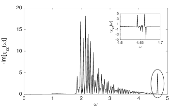
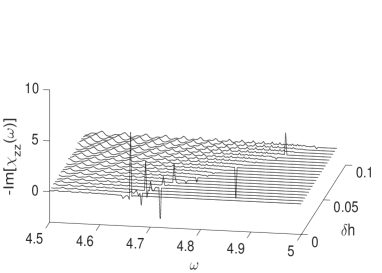
Figure 1: Top panel: $\mathrm{Im}(\chi(\omega))$ for a chain of $N=200$ sites at a non-equilibrium critical point. The ellipsis emphasizes the peak related to the closing of the Liouvillian gap $\Delta$. In the inset a zoom of the region around the peak shows the non-monotonic behavior of the peak with $\omega$. Bottom panel, a region of frequencies around the peak location is shown for different fields $\delta h$ close to the critical point $h=h_{c}+\delta h$ (with $h_{c}=1-\gamma^{2}$) for $N=200$ sites. Peaks are presents also sufficiently close to the critical point however there is a non-monotonic behavior as described in the main text. Other parameters are $\gamma=0.8$, $\Gamma_{1}^{L}=0.3,\,\Gamma_{2}^{L}=0.1$, $\Gamma_{1}^{R}=0.3,\,\Gamma_{2}^{R}=0.2$.

V.1 Dissipative $XY$ spin-chain

We will now study a specific example of quasi-free open system. Namely we consider the model introduced in (Prosen, 2008; Prosen and Pižorn, 2008) of an $XY$ spin-chain with thermal magnetic baths acting at the ends of the chain. The model is given by Eq. (18) with Hamiltonian

$$H=\sum_{n=1}^{N-1}\left(\frac{1+\gamma}{2}\sigma_{n}^{x}\sigma_{n+1}^{x}+\frac{1-\gamma}{2}\sigma_{n}^{y}\sigma_{n+1}^{y}\right)+\sum_{n=1}^{N}h\sigma_{n}^{z}\,,$$

and the following four Lindblad operators

$$L_{1}=\sqrt{\Gamma_{1}^{L}}\sigma_{1}^{-}, \,\,L_{3}=\sqrt{\Gamma_{1}^{R}}\sigma_{N}^{-},$$

$$L_{2}=\sqrt{\Gamma_{2}^{L}}\sigma_{1}^{+}, \,\,L_{4}=\sqrt{\Gamma_{2}^{R}}\sigma_{N}^{+},$$

where $\sigma_{n}^{\pm}=(\sigma_{n}^{x}\pm i\sigma_{n}^{y})/2$ and $\Gamma_{1,2}^{L,R}$ are positive constants related to the baths temperature at the ends. Namely $\Gamma_{2}^{\ell}/\Gamma_{1}^{\ell}=\exp(-2h/T_{\ell})$ for $\ell=L,R$. In the thermodynamic limit the model has a critical “line” $h_{c}^{2}=(1-\gamma^{2})^{2}$ where the correlations $\langle\sigma_{n}^{z}\sigma_{n+r}^{z}\rangle$ decay algebraically as $r^{-4}$. Outside criticality the decay is exponential with a correlation length $\xi=1/4\mathrm{arccosh}(h/h_{c})]$, hence $\xi$ diverges with a mean-field exponent, $\xi\sim\left|h-h_{c}\right|^{-1/2}$, as the critical point is approached.

The matrix $X$, as can be seen from Eq. (38), plays an analogous role as the Hamiltonian in this open system setting. In our numerical simulations we verified that $X$ could always be diagonalized. In this case the Lindblad generator can be cast in the following normal form $\mathcal{L}_{0}=\sum_{k}\lambda_{k}d_{k}^{\times}d_{k}$ where the operators $d_{k}^{\times}\neq d_{k}^{\dagger}$ but otherwise satisfy canonical anticommutation relations such that $d_{k}^{\times}d_{k}$ are non-hermitean number operators. As proven in (Prosen, 2008) the non-equilibrium steady state is unique iff $\lambda_{k}\neq 0$ for all $k$. In this case the convergence to the NESS is exponential with a rate given by the “gap” $\Delta=2\min_{k}\{-\mathrm{Re}(\lambda_{k})\}$. Such non-equilibrium phase transition are also characterized by a different scaling to zero with $N$ of the dissipative gap $\Delta$ (Prosen and Pižorn, 2008). Namely, as $N\to\infty$, one has $\Delta(N)\sim N^{-5}$ at the critical points whereas $\Delta(N)\sim N^{-3}$ elsewhere.

At the critical point we numerically observe a multitude of levels whose real part is going to zero. This seems to be analogous to standard, Hamiltonian, second order phase transitions where an extensive number of energy gaps go to zero in the thermodynamic limit. In our simulations we observe this feature at the edge of the spectrum i.e. for $\omega\approx\pm 2\max\mathrm{Im}(\lambda_{k})$. Assume then, that for a certain number of $k$’s one has, approximately $\lambda_{k}\approx\sigma-i\rho$ with $|\sigma|\ll 1$. The denominator in Eq. (49) gives rise to a contribution of the form $[2\sigma-i(\omega-2\rho)]/[(\omega-2\rho)^{2}+4\sigma^{2}]$, in other words we expect a strong, Lorentzian, peak at $\omega\approx 2\rho$. This argument finds indeed numerical confirmation as can be seen from figure 1. Such peaks are present in a quasi-critical region, sufficiently close to the (out-of-equilibrium) critical point. The size and scaling properties of such peaks are, however, difficult to predict. For example the peak hight is not necessarily increasing with systems size. The reason is that the numerator $[\hat{\mathsf{A}^{T}}]_{k,q}[\check{C}_{1}]_{q,k}$ in Eq. (49) not only does not have a definite sign but is in fact complex. The overall contribution to $\mathrm{Im}(\chi(\omega))$ is a linear combination of peaked Lorentzian with coefficients of possibly different sign. This effect can be appreciated in Fig. 1 bottom panel where peaks are shown for a region of field close to criticality. As a function of the external field, peaks change sign and may even disappear completely as a consequence of destructive interference. In Fig. 2 we also plot the single particle MHR, Eq. (50) and compare it with the LDS. The MHR reveals similar features as $\mathrm{Im}[\chi_{zz}(\omega)]$ albeit possibly more pronounced. Finally we consider perturbation of purely dissipative character, i.e. we set $\mathcal{L}_{1}=\mathcal{L}_{0}+i\left[H,\bullet\right]$. The results are shown in Fig. 3

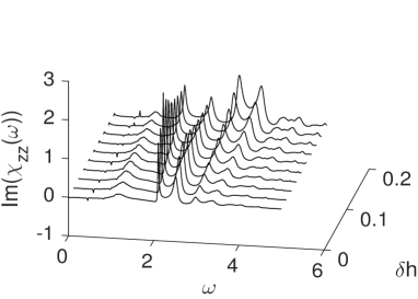
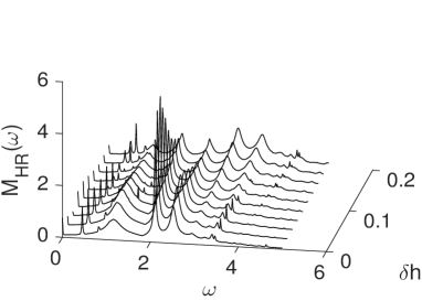
Figure 2: Comparison between LDS and the single particle MHR Eq. (50). Top panel: imaginary LDS in frequency domain computed using Eq. (49). Bottom panel: single particle MHR $\mathsf{M}_{\mathrm{HR}}(\omega)$ as given by Eq. (50). The system’s size is $N=14$ and the external field is $h=h_{c}+\delta h$, where $h_{c}=1-\gamma^{2}$ is the critical field. Other parameters as in Fig. 1.

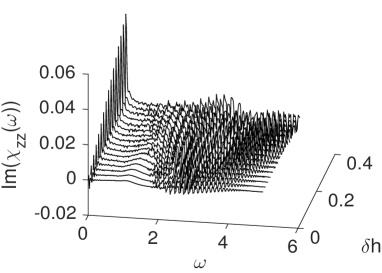
Figure 3: LDS for a purely dissipative perturbation. Size is $N=100$. Other parameters as in Fig. 1.

VI Conclusions

In this paper we discussed the extension of Kubo linear response theory to open quantum systems whose dynamics is described by a master equation generating a semi-group of contractive dynamical maps.

The theory parallels the standard closed case but some important differences arise. For example, for generators with a unique steady state, the generalization of the thermal susceptibility becomes now equal to the $\omega=0$ complex admittance. This is known not to be the case in the unitary setting (Kubo, 1957). Moreover for a class of hermitean dynamical maps we have shown that the diagonal response functions are identically vanishing. We derived exact expressions for the linear dynamical response functions for generalized dephasing, Davies generators, and integrable, quasi-free master equation. We introduced the observable-free notion of maximal harmonic response and computed it explicitly for a single qubit.

In the quasi-free case we concentrated the analysis close to the dynamical phase transition points which are known to take place in these systems. It is found that a signature of such dynamical phase transitions shows up as a peak in the imaginary part of the admittance at the edge of the spectrum.

Applications of our dynamical response theory to a variety of physically relevant systems as well as its extension to wider class of open quantum system dynamics e.g., non-Markovian, clearly deserve future investigations.