An Optimized Ion Trap Geometry to Measure Quadrupole Shifts of ¹⁷¹Yb⁺ Clocks

Abstract

We propose a new ion-trap geometry to carry out accurate measurements of the quadrupole shifts in the ¹⁷¹Yb-ion. This trap will produce nearly ideal harmonic potential where the quadrupole shifts due to the anharmonic components can be reduced by four orders of magnitude. This will be useful to reduce the uncertainties in the clock frequency measurements of the $6s~{}{{}^{2}}S_{1/2}\rightarrow 4f^{13}6s^{2}~{}{{}^{2}}F_{7/2}$ and $6s~{}{{}^{2}}S_{1/2}\rightarrow 5d~{}{{}^{2}}D_{3/2}$ transitions, from which we can deduce precise values of the quadrupole moments ($\Theta$s) of the $4f^{13}6s^{2}~{}{{}^{2}}F_{7/2}$ and $5d~{}{{}^{2}}D_{3/2}$ states. Moreover, it may be able to affirm validity of the measured $\Theta$ value of the $4f^{13}6s^{2}~{}{{}^{2}}F_{7/2}$ state where three independent theoretical studies defer almost by one order in magnitude from the measurement. We also perform calculations of $\Theta$s using the relativistic coupled-cluster (RCC) method. We use these $\Theta$ values to estimate quadrupole shift that can be measured in our proposed ion trap experiment.

I Introduction

Advances in trapping and laser control of a single ion ABauch_RPP_2002 ; Poli_Nuovo_2013 ; Takamoto_CRphys_2015 began a new era for the frequency standards in the optical range, which are aimed to achieve a fractional accuracy of $10^{-16}-10^{-18}$. Worldwide a number of ions, such as, ¹⁹⁹Hg⁺ Rosenband_Science_2008 , ¹⁷¹Yb⁺ Gill_IEEE_2003 ; Godun_PRL_2014 ; Tamm_PRA_2009 ; Huntemann_PRL_2012 ; Huntemann_PRL_2014 , ¹¹⁵In⁺ Wang_OC_2007 , ⁸⁸Sr⁺ Dube_PRA_2013 ; Barwood_PRL_2014 , ⁴⁰Ca⁺ Huang_APB_2014 ; Kajita_PRA_2005 , ²⁷Al⁺ Chou_PRL_2010 etc. have been undertaken in the experiments to attain such promising optical frequency standards. Among them ¹⁷¹Yb⁺ is unique in the sense that it has three potential optical transitions that can be used for clocks Nandy_PRA_2014 . Out of these there are two narrow $6s~{}{{}^{2}}S_{1/2}(F=0,m_{F}=0)\rightarrow 5d~{}{{}^{2}}D_{3/2}(F=2,m_{F}=0)$ Webster_IEEE_2010 ; Tamm_PRA_2014a , $6s~{}{{}^{2}}S_{1/2}(F=0,m_{F}=0)\rightarrow 5d~{}{{}^{2}}D_{5/2}(F=2,m_{F}=0)$ Roberts_PRA_1999 quadrupole (E2) transitions and an ultra-narrow $6s~{}{{}^{2}}S_{1/2}(F=0,m_{F}=0)\rightarrow 4f^{13}6s^{2}~{}{{}^{2}}F_{7/2}(F=3,m_{F}=0)$ octupole (E3) transition King_NJP_2012 ; Huntemann_PRL_2014 with their respective wavelengths at 435.5 nm, 411 nm and 467 nm. The transitions at the wavelengths 435.5 nm and 467 nm with low systematic shifts are the most suitable ones for precision frequency standards owing to their extremely small natural line-widths 3.02 Hz and 1 nHz, respectively. Their precisely measured transition frequencies $\nu_{o}$ have already been reported as $688\,358\,979\,309\,306.62(73)$ Hz Tamm_PRA_2014a and $688\,358\,979\,309\,310(9)$ Hz Webster_IEEE_2010 for the E2-transition and $642\,121\,496\,772\,645.36(39)$ Hz Huntemann_PRL_2014 and $642\,121\,496\,772\,646.22(67)$ Hz King_NJP_2012 for the E3-transition. These two transitions are endorsed by the international committee for weight and measures (CIPM) for secondary representation of standard international (SI) second owing to their least sensitive to the external electromagnetic fields. Other than being a potential candidate for frequency standards, Yb⁺ is also being considered for studying parity non-conservation effect Dzuba_PRA_2011 ; Sahoo_PRA_2011 , violation of the Lorenz symmetry VADzuba_Arxiv_2015 , searching for possible temporary variation of the fine structure constant Dzuba_PRA_2003 ; Dzuba_PRA_2008 etc.

In an atomic clock, the measured frequency of the interrogated transition is always different than its absolute value due to the systematics. The net frequency shift depends upon many environmental factors and experimental conditions, which may or may not be canceled out at the end. Thus, they need to be accounted to establish accurate frequency standards. Careful design of the ion traps are also very important for minimizing the systematics caused by the environmental factors Nisbet_Arxiv_2015 . Electric quadrupole shift is one of the major systematics when the states associated with the clock transition have finite quadrupole moments ($\Theta$s). In the ¹⁷¹Yb⁺ ion, the experimentally measured $\Theta$ value of the $5d~{}{{}^{2}}D_{3/2}$ state Schneider_PRL_2005 is 50 times larger than the $4f^{13}6s^{2}~{}{{}^{2}}F_{7/2}$ state. A recent theoretical study suggests a more precise $\Theta$ value of the $5d~{}{{}^{2}}D_{3/2}$ state Nandy_PRA_2014 . Similarly, three independent theoretical investigations Blythe_JPB_2003 ; Porsev_PRA_2012 ; Nandy_PRA_2014 shows very large disagreements than the measured Huntemann_PRL_2012 $\Theta$ value of the $4f^{13}6s^{2}~{}{{}^{2}}F_{7/2}$ state. Therefore, it is imperative to carry out further investigations to attain more precise and reliable values of $\Theta$s and probe the reason for the anomalies between the calculated and experimental results. Here we also perform another calculation using the relativistic coupled-cluster (RCC) method to evaluate the $\Theta$ values of the $5d~{}{{}^{2}}D_{3/2}$ and $4f^{13}6s^{2}~{}{{}^{2}}F_{7/2}$ states to use them in the present analysis. We also analyze in detail about the suitable confining potentials, electric fields and field gradients that can create a nearly ideal quadrupole trap condition for carrying out precise measurements of the $\Theta$ values. Using these inputs we estimate typical values of the quadrupole shifts of the $6s~{}{{}^{2}}S_{1/2}(F=0,m_{F}=0)\rightarrow 5d~{}{{}^{2}}D_{3/2}(F=2,m_{F}=0)$ and $6s~{}{{}^{2}}S_{1/2}(F=0,m_{F}=0)\rightarrow 4f^{13}6s^{2}~{}{{}^{2}}F_{7/2}(F=3,m_{F}=0)$ clock transitions considering a number of ion trap geometries and discuss their possible pros and cons to make an appropriate choice. This analysis identifies a suitable geometry of the end cap ion trap to measure $\Theta$s of the $5d~{}{{}^{2}}D_{3/2}$ and $4f^{13}6s^{2}~{}{{}^{2}}F_{7/2}$ states of Yb⁺ which is being developed at the National Physical Laboratory (NPL), India ARastogi_Mapan_2015 ; SDe_currentsc_2014 .

II Electric Quadrupole Shift

Electric quadrupole shift $\Delta\nu_{Q}$ to an atomic state with angular momentum $F$ arises due to the interaction of the quadrupole moment $\Theta(\gamma,F)$ with an applied external electric field gradient $\nabla E$, where $\gamma$ represents for the other quantum numbers of the state. A non-zero atomic angular momentum results in a non-spherical charge distribution, thus atom acquires higher order moments. Following this it is advantageous to choose states with $J<1$ or $F<1$ in a clock transition for which $\Theta=0$. However, the excited states of the $6s~{}{{}^{2}}S_{1/2}(F=0,m_{F}=0)\rightarrow 5d~{}{{}^{2}}D_{3/2}(F=2,m_{F}=0)$ and $6s~{}{{}^{2}}S_{1/2}(F=0,m_{F}=0)\rightarrow 4f^{13}6s^{2}~{}{{}^{2}}F_{7/2}(F=3,m_{F}=0)$ clock transitions have $J=3/2;F=2$ and $J=7/2;F=3$ resulting in nonzero quadrupole shifts. These shifts can be estimated by calculating the expectation value of the Hamiltonian given by Ramsey_oxford_1956

$$H_{Q}=\mbox{\boldmath$\nabla$}E\cdot\mbox{\boldmath$\Theta$}(\gamma,F)=\sum^{2}_{q=-2}(-1)^{q}\nabla E_{q}\Theta_{-q},$$ (1)

where ranks of the $\mbox{\boldmath$\nabla$}E$ and $\Theta$ tensors are two and their components are indicated by subscript $q$. The expectation value of $H_{Q}$ in reduced form can be expressed as Itano_Nist_2000

$$\langle\gamma JFm_{F}|H_{Q}|\gamma JFm_{F}\rangle = \Theta(\gamma,J)\,\mathcal{F}_{Q}(I,J,F,m_{F})$$ (2)

$$\times\sum_{q=-2}^{2}\nabla E_{q}D_{0q},$$

where $m_{F}$ is the magnetic quantum number, $D_{0q}$ are the rotation matrix elements of the projecting components of $\nabla E$ in the principal axis frame that are used to convert from the trap axes to the lab frame Edmonds_princeton_1974 , $\Theta(\gamma,J)$ is the quadrupole moment of the atomic state with angular momentum $J$ and

$$\mathcal{F}_{Q}=(-1)^{I+J+F}(2F+1)\left(\begin{array}[]{ccc}F&2&F\\ -m_{F}&0&m_{F}\\ \end{array}\right)$$ (5)

$$\times{\left(\begin{array}[]{ccc}J&2&J\\ -J&0&J\\ \end{array}\right)}^{-1}\left\{\begin{array}[]{ccc}J&2&J\\ F&I&F\\ \end{array}\right\}.$$ (10)

Here the quantities within $(\,)$ and $\{\,\}$ represent the $3j$ and $6j$-coefficients, respectively. Both the excited states of the above mentioned clock transitions acquire $\mathcal{F}_{Q}=1$. Due to axial symmetry of the trap, the frequency shift contributions from $D_{0\pm 1}$ cancel with each other, thus finite contributions comes only from the $D_{00}=(3\cos^{2}\theta-1)/2$ and $D_{0\pm 2}=\sqrt{3/8}\sin^{2}\theta(\cos 2\phi\mp i\sin 2\phi)$ components, for the Euler’s angles $\theta$ and $\phi$. In this work, we use our calculated $\Theta$ values for the $5d^{2}D_{3/2}(F=2)$ and $4f^{13}6s^{2}~{}^{2}F_{7/2}(F=3)$ states to find out the optimum electrode geometries that can produce nearly-ideal quadrupole confining potentials after interacting with the resultant electric field gradients of the non-ideal multipole potentials $\Phi(x,y,z)=\sum_{k=1}^{\infty}\Phi^{(k)}$ with the order of multipole $k$ of the effective trapping potentials.

III Methods for calculation

To calculate atomic state wave functions for the determination of the $\Theta(\gamma,J)$ values we adopt the Bloch’s approach lindgren . Following this approach we express the wave function $|\Psi_{v}\rangle$ of the $5d~{}{{}^{2}}D_{3/2}$ state with the valence orbital $v$ in the $5d_{3/2}$ orbital as

$$|\Psi_{v}\rangle=\Omega_{v}|\Phi_{v}\rangle$$ (11)

and the wave function $|\Psi_{a}\rangle$ of the $4f^{13}6s^{2}~{}{{}^{2}}F_{7/2}$ state with the valence orbital $a$ in the $4f_{7/2}$ orbital as

$$|\Psi_{a}\rangle=\Omega_{a}|\Phi_{a}\rangle$$ (12)

of the Yb⁺ ion, where $\Omega_{v}$ and $\Omega_{a}$ are the wave operators for the corresponding reference states $|\Phi_{v}\rangle$ and $|\Phi_{a}\rangle$, respectively. We use two different ways to construct these reference states. For the computational simplification we choose the working reference states as the Dirac-Hartree-Fock (DHF) wave functions of the closed-shell configurations (denoted by $|\Phi_{0}^{v/a}\rangle$) in place of the above mentioned respective actual reference states $|\Phi_{v}\rangle$ and $|\Phi_{a}\rangle$ having open valence orbitals. In our calculations we have obtained $|\Phi_{0}^{v}\rangle$ for the $[4f^{14}]$ configuration, while $|\Phi_{0}^{a}\rangle$ is calculated with the $[4f^{14}]6s^{2}$ configuration. Then, the actual reference states are obtained by appending the valence orbital $v=5d_{3/2}$ and removing the spin partner of the valence orbital $a=4f_{7/2}$ of the respective references. In the second quantization formalism, it is given as

$$|\Phi_{v}\rangle=a_{v}^{\dagger}|\Phi_{0}^{v}\rangle\ \ \ \text{and}\ \ \ |\Phi_{a}\rangle=a_{a}|\Phi_{0}^{a}\rangle.$$ (13)

We employ the Dirac-Coulomb Hamiltonian for the calculations which in the atomic unit (a.u.) is given by

$$H = \sum_{i}\left[c\mbox{\boldmath$\alpha$}_{i}\cdot\textbf{p}_{i}+(\beta_{i}-1)c^{2}+V_{n}(r_{i})+\sum_{j>i}\frac{1}{r_{ij}}\right],\ \ \ \ \ \$$ (14)

with $\alpha$ and $\beta$ are the usual Dirac matrices and $V_{n}(r)$ represents the nuclear potential.

In a perturbative procedure, $\Omega_{v/a}$ can be expressed as

$$\Omega_{v/a}=1+\chi_{0}^{v/a}+\chi_{v/a}\equiv\Omega_{0}^{v/a}+\chi_{v/a},$$ (15)

where $\chi_{0}^{v/a}$ and $\chi_{v/a}$ are responsible for carrying out excitations from $|\Phi_{0}^{v/a}\rangle$ due to the residual interaction $V_{r}=H-H_{0}$ for the DHF Hamiltonian $H_{0}$. In a series expansion they are given as

$$\chi_{0}^{v/a}=\sum_{k}\chi_{0}^{v/a(k)}\ \ \text{and}\ \ \chi_{v/a}=\sum_{k}\chi_{v/a}^{(k)},$$ (16)

where the superscript $k$ refers to the number of times $V_{r}$ is considered in the many-body perturbation theory (MBPT(k) method). The k^th order amplitudes for the $\chi_{0}^{v/a}$ and $\chi_{v/a}$ operators are obtained by solving the following equations lindgren

$$[\chi_{0}^{v/a(k)},H_{0}]P_{0}^{v/a} = Q_{0}^{v/a}V_{r}(1+\chi_{0}^{v/a(k-1)})P_{0}^{v/a}\ \ \ \ \$$ (17)

and

$$[\chi_{v/a}^{(k)},H_{0}]P_{v/a} = Q_{v/a}V_{r}(1+\chi_{0}^{v/a(k-1)}$$ (18)

$$+ \chi_{v/a}^{(k-1)})P_{v/a}-\sum_{m=1}^{k-1}\chi_{v/a}^{(k-m)}P_{v/a}V_{r}$$

$$\times (1+\chi_{0}^{v/a(m-1)}+\chi_{v/a}^{(m-1)})P_{v/a},$$

where the projection operators are defined as $P_{0}^{v/a}=|\Phi_{0}^{v/a}\rangle\langle\Phi_{0}^{v/a}|$, $Q_{0}^{v/a}=1-P_{0}^{v/a}$, $P_{v/a}=|\Phi_{v/a}\rangle\langle\Phi_{v/a}|$ and $Q_{v/a}=1-P_{v/a}$. The exact energies for the states having the closed-shell and open-shell configurations are evaluated using the effective Hamiltonians given by

$$H_{0}^{eff,v/a}=P_{0}^{v/a}H\Omega_{0}^{v/a}P_{0}^{v/a}$$ (19)

and

$$H_{v/a}^{eff}=P_{v/a}H\Omega_{v/a}P_{v/a}.$$ (20)

Table 1: Demonstration of trends in the $\Theta$ values (in a.u.) from lower to higher order methods. Our calculations are compared with the values available from other calculations and the experimental results. The estimated final values are shown in bold fonts. Uncertainties to these values are also quoted separately.

Method	$4f^{14}5d\,\rm{{}^{5}D_{3/2}}$	$4f^{13}6s^{2}\,\rm{{}^{2}F_{7/2}}$
DHF	2.504	$-0.258$
MBPT(2)	2.049	$-0.344$
LCCSD	2.028	$-0.230$
CCSD(2)	2.060	$-0.208$
CCSD	2.061	$-0.223$
CCSDex	2.079	${\bf-0.224}$
Uncertainty	$\pm 0.008$	$\pm 0.010$
Others	2.174a	$-0.22^{b}$
	2.157c	$-0.20^{d}$
	2.068(12)e	$-0.216(20)^{e}$
Experiment	2.08(11)f	$-0.041(5)^{g}$

References:	aItano_PRA_2006 .
	bBlythe_JPB_2003 .
	cLatha_PRA_2007 .
	dPorsev_PRA_2012 .
	eNandy_PRA_2014 .
	fSchneider_PRL_2005 .
	gHuntemann_PRL_2012 .

In the RCC theory framework, the wave functions of the considered states are expressed as (e.g. see Nandy_PRA_2014 ; Nandy_PRA_2013 )

$$|\Psi_{v}\rangle=e^{T^{v}}\{1+S_{v}\}|\Phi_{v}\rangle$$ (21)

and

$$|\Psi_{a}\rangle=e^{T^{a}}\{1+R_{a}\}|\Phi_{a}\rangle,$$ (22)

where $T^{v}$ and $T^{a}$ excite the core electrons from the new reference states $|\Phi_{0}^{v}\rangle$ and $|\Phi_{0}^{a}\rangle$, respectively, to account for the electron correlation effects. The $S_{v}$ and $\left(e^{T^{v}}-1\right)S_{v}$ operators excite electrons from the valence and valence with core orbitals from $|\Phi_{v}\rangle$. Similarly, the $R_{a}$ and $\left(e^{T^{a}}-1\right)R_{a}$ operators excite electrons from the valence and valence with core orbitals from $|\Phi_{a}\rangle$. In this work we have considered only the singles and doubles excitations in the RCC theory (CCSD method), which are identified by the RCC operators with the subscripts $1$ and $2$, respectively, as

$$T^{v/a} = T_{1}^{v/a}+T_{2}^{v/a}$$

$$S_{v} = S_{1v}+S_{2v}$$

$$\text{and}\ \ \ R_{a} = R_{1a}+R_{2a}.$$ (23)

When only the linear terms are retained in Eqs. (21) and (22) with the singles and doubles excitations approximation in the RCC theory, we refer it to as LCCSD method. The amplitudes of the above operators are evaluated by the equations

$$\langle\Phi_{0}^{v/a,*}|\overline{H}_{N}^{v/a}|\Phi_{0}^{v/a}\rangle = 0$$ (24)

$$\langle\Phi_{v}^{*}|\big{(}\overline{H}_{N}^{v}-\Delta E_{v}\big{)}S_{v}|\Phi_{v}\rangle = -\langle\Phi_{v}^{*}|\overline{H}_{N}^{v}|\Phi_{v}\rangle$$ (25)

and

$$\langle\Phi_{a}^{*}|\big{(}\overline{H}_{N}^{a}-\Delta E_{a}\big{)}R_{a}|\Phi_{a}\rangle = -\langle\Phi_{a}^{*}|\overline{H}_{N}^{a}|\Phi_{a}\rangle,$$ (26)

where $|\Phi_{0}^{v/a}\rangle$ and $|\Phi_{v/a}^{*}\rangle$ are the excited state configurations with respect to the DHF states $|\Phi_{0}^{v/a}\rangle$ and $|\Phi_{v/a}\rangle$, respectively, and $\overline{H}_{N}^{v/a}=\big{(}H_{N}e^{T^{v/a}}\big{)}_{c}$ with subscript $c$ representing for the connected terms only. Here $\Delta E_{v}=H_{v}^{eff}-H_{0}^{eff,v}$ and $\Delta E_{a}=H_{a}^{eff}-H_{0}^{eff,a}$ are the attachment energy of the electron in the valence orbital $v$ and ionization potential of the electron in the orbital $a$, respectively. Following Eqs. (19) and (20), $\Delta E_{v/a}$ are evaluated as

$$\Delta E_{v}=\langle\Phi_{v}|\overline{H}_{N}^{v}\left\{1+S_{v}\right\}|\Phi_{v}\rangle$$ (27)

and

$$\Delta E_{a}=\langle\Phi_{a}|\overline{H}_{N}^{a}\left\{1+R_{a}\right\}|\Phi_{a}\rangle.$$ (28)

To improve quality of the wave functions, we use experimental values of $\Delta E_{v/a}$ instead of the calculated values in the CCSD method and refer to the approach as CCSD${}_{\text{ex}}$ method. This is obviously better than the approach to improve the $E_{v/a}$ values by incorporating contributions from the important triple excitations in a perturbative approach in the CCSD method (CCSD(T) method) that was employed in Nandy_PRA_2014 ; Nandy_PRA_2013 .

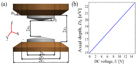
Figure 1: (a) Our proposed electrode assembly of the end-cap trap with $2z_{0}=0.7$ mm, $2z_{2}\approx 1.0$ mm, $2r_{1}=1$ mm, $2r_{2}=1.4$ mm, $2r_{3}=2$ mm, $\theta_{i}=10^{\circ}$ and $\theta_{o}=45^{\circ}$. (b) Variation of the trap depth as a function of dc voltage $U$ for a fixed radio-frequency $\omega_{rf}$ and an ac voltage $V$.

After obtaining amplitudes of the MBPT and RCC operators using the equations described above, the $\Theta$ values of the considered states are evaluated using the expression

$$\frac{\langle\Psi_{v/a}|\Theta|\Psi_{v/a}\rangle}{\langle\Psi_{v/a}|\Psi_{v/a}\rangle} = \frac{\langle\Phi_{v/a}|\Omega_{v/a}^{\dagger}\Theta\Omega_{v/a}|\Phi_{v/a}\rangle}{\langle\Phi_{v/a}|\Omega_{v/a}^{\dagger}\Omega_{v/a}|\Phi_{v/a}\rangle}.$$ (29)

This gives rise to a finite number of terms for the MBPT(2) and LCCSD methods, but it involves two non-terminating series in the numerator and denominator, which are $e^{T^{v/a\dagger}}\Theta e^{T^{v/a}}$ and $e^{T^{v/a\dagger}}e^{T^{v/a}}$ respectively, in the CCSD method. We account contributions from these non-truncative series by adopting iterative procedures as described in our previous works Sahoo_PRA_2015 ; Singh_PRA_2015 . We also give results considering only the linear terms of Eq. (29) that appear exactly in the LCCSD method, but using amplitudes of the RCC operators from the CCSD method (refer it as CCSD⁽²⁾ method). Therefore from the differences in the results between the LCCSD and CCSD methods, one can infer about the importance of the non-linear terms in the calculations of the wave functions; while from the differences in the results between the CCSD⁽²⁾ and CCSD methods, it will signify the roles of the non-linear effects appearing in Eq. (29) for the estimations of the $\Theta$ values.

We present $\Theta$ values of the $4f^{14}5d\,\rm{{}^{5}D_{3/2}}$ and $4f^{13}6s^{2}\,\rm{{}^{2}F_{7/2}}$ states of Yb⁺ in Table 1 from various methods as described above. We also compare our results with the other calculations and available experimental values. We consider results from the CCSD${}_{\text{ex}}$ method as our recommended values as this method accounts more physical effects. We have also estimated uncertainties to the CCSD${}_{\text{ex}}$ results by estimating neglected contributions due to truncation in the basis functions and from the omitted correlation effects mainly that could arise through the triply excited configurations. We had also presented these values using the CCSD method in our previous work Nandy_PRA_2014 , however considering only the important non-linear terms from the $e^{T^{v/a\dagger}}\Theta e^{T^{v/a}}$ and $e^{T^{v/a\dagger}}e^{T^{v/a}}$ non-truncative series of Eq. (29). As said before these series are solved iteratively to include infinity numbers of terms in this work. Again, we have removed uncertainties due to the calculated energies that enter into the amplitude solving Eq. (25) of the CCSD method by using the experimental energies.

IV Ion Trap Induced Shift

We plan to employ a modified Paul trap Paul_Rev_1990 of end cap geometry as shown in Fig.1(a). In reality, such traps are not capable of producing pure quadrupole potential $\Phi^{(2)}$ due to geometric modifications of the hyperbolic electrode, machining inaccuracies and misalignments. On the other hand, precision measurements with ions stored in a non-ideal trap, the anharmonic components of the potential $\Phi^{(k>2)}(x,y,z)$ are non-negligible due to the fact that they change ion dynamics and also affect the systematics. For minimizing such effects several groups, such as, NPL UK Schrama_Optcomm_1993 , NRC Canada Dube_PRA_2013 and PTB Germany Stein_Thesis_2010 ; PTB_arxiv_2015 have come up with different end cap trap designs for establishing single ion frequency standards. Here we aim to identify a new end cap trap geometry in which the trap induced quadrupole shift can be minimized. This trap can also add minimum anharmonicity to the confining potential and small micromotions Our_calculation . In a cylindrically symmetric trap as shown in Fig.1(a), only the even order multipoles contribute.

Here, in order to estimate quality of the trap potentials we consider $k$ up to 10 since amplitudes of $\Phi^{(k)}$ fall drastically at higher $k$. The tensor components of $\nabla E$ for each multipole potential $\Phi^{(k)}$ are opted from their electric field components $E_{x,y,z}$. The corresponding fractional quadrupole shift $\Delta\nu_{Q}/\nu_{0}$ at each $k$ is estimated from Eq. (2). The variation of $\Delta\nu_{Q}/\nu_{0}$ for all multipole potentials up to $k=10$ at two different distances from the trap center are estimated for the E2 and E3-clock transitions, which are shown in Fig. 2(a-b). The reported experimental values of the quadrupole shifts for these two transitions are also depicted in the same figure for the comparison.

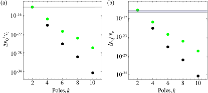
Figure 2: (Color online) Fractional electric quadrupole shifts due to the multipoles up to $k=10$ for the (a) E2 and (b) E3 transitions, when the ion is off centered by a distance 10 $\mu$m (black) and 100 $\mu$m (green), respectively. The harmonic potential gives a spatially independent $|\Delta\nu_{Q}/\nu_{o}|$. The reported fractional accuracies $5\times 10^{-16}$ for the E2-transition Tamm_PRA_2009 , $7.1\times 10^{-17}$ Huntemann_PRL_2012 and $1\times 10^{-15}$ King_NJP_2012 for the E3-transition are indicated by a gray line in (a) and by a gray band in (b), respectively.

The dominating perturbation of $\Phi^{(2)}$ arises from the octupole term $\Phi^{(4)}$ which may largely affect the quadrupole shift of the trapped ion frequency standards due to wrong choice of the electrode geometry. As an example, we simplify the analysis considering $\Phi(x,y,z)\simeq\Phi^{(2)}+\Phi^{(4)}$ since other higher orders are less significant for the quadrupole shift (Fig. 2). In the absence of any asymmetries the trap potential can be written as

$$\Phi(x,y,z) = \frac{V_{T}(t)}{2{R}^{2}}\bigg{[}c_{2}(2z^{2}-x^{2}-y^{2})-\frac{c_{4}}{{R}^{2}}(3x^{4}+3y^{4}$$ (30)

$$+8z^{4}-24x^{2}z^{2}-24y^{2}z^{2}+6x^{2}y^{2})\bigg{]}$$

where, $R=\sqrt{{{r_{0}}^{2}}/2+{z_{0}}^{2}}$ and $V_{T}(t)=U+V\cos(\omega_{rf}t)$ that depends on the dc and rf components of the trapping voltages with amplitudes $U$ and $V$, respectively. The dimensionless coefficients $c_{2}$ and $c_{4}$ depend on the electrode geometry. Here we consider $|x|=|y|=r$, since the trap is axially symmetric. The harmonic part of the potential can produce the restoring force on the ion and the resultant axial trap depth yields $D_{z}(U,V,\omega_{rf})=U/2+m{z_{o}}^{2}{\omega}^{2}_{rf}{q_{z}}^{2}/16Q$ Werth_springer_2010 where $q_{z}=-16QVc_{2}/mR^{2}{\omega}^{2}_{rf}$ and $Q$ and $m$ are the charge and mass of the ion, respectively. As an example, in Fig. 1 (b) we show the variation of $D_{z}$ with $U$ for fixed values $V=500$ V and $\omega_{rf}=2\pi\times 12$ MHz, respectively. Since the first order quadrupole shift from the rf averages to zero and its second order is also zero for $\rm{{}^{171}Yb^{+}}$ Schneider_PRL_2005 , we estimate the shift considering $U=10$ V. The quadrupole shift as given by $\sum_{q}\nabla E_{q}D_{0q}$ results to $2V_{T}c_{2}[D_{00}-D_{02}/\sqrt{6}]$ due to the harmonic part of the potential and it is constant within the trapping volume. The spatial dependency comes from the higher orders, for example $\Phi^{(4)}$ results to a quadrupole shift of $12V_{T}c_{4}[4z^{2}(D_{00}-D_{02}/\sqrt{6})-r^{2}(2D_{00}-\sqrt{3/2}D_{02})]$.

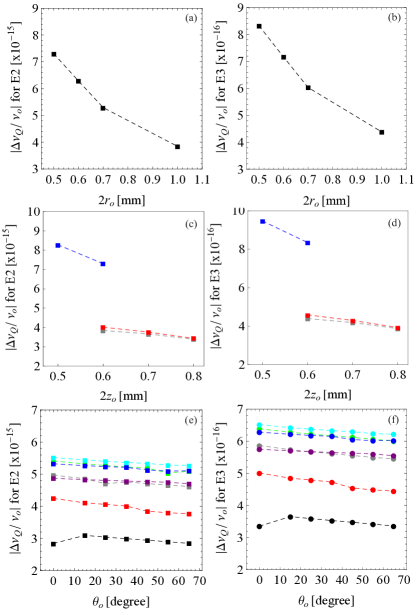
Figure 3: (Color online) Fractional electric quadrupole shift for the E2 and E3-clock transitions corresponding to the different geometrical parameters: (a, b) diameter $2r_{o}$ of the inner electrode; (c, d) tip-to-tip separation $2z_{o}$ of the inner electrodes; and (e, f) angles $\theta_{o}$ at which the outer electrodes are machined. Each figure consists of a set of plots for angles of the inner electrode $\theta_{i}$, which are at $0^{\circ}$ (black), $10^{\circ}$ (red), $20^{\circ}$ (gray), $30^{\circ}$ (green), $40^{\circ}$ (cyan), $50^{\circ}$ (blue) and $60^{\circ}$ (purple). The dashed line connects data points for the fixed values of $\theta_{i}$ and considering $2r_{o}=1$ mm and $2z_{o}=0.7$ mm for all of them. Each figure consists of a set of plots for the angles of the inner electrode $\theta_{i}$, which are at $0^{\circ}$ (black), $10^{\circ}$ (red), $20^{\circ}$ (gray), $30^{\circ}$ (green), $40^{\circ}$ (cyan), $50^{\circ}$ (blue) and $60^{\circ}$ (purple).

Strength of the multipole potentials depend on $c_{k}$ as given in Eq. (30). The magnitudes of $c_{k}$ depend on the geometric parameters of the trap electrodes, such as radius $r_{o}$, angle $\theta_{i}$ of the electrode carrying rf (that is the inner electrode), inside and outside radii $r_{1}$ and $r_{2}$, angle $\theta_{o}$ of the dc carrying electrode (that is the outer electrode) which is coaxial to the inner one and also their mutual tip-to-tip separations $2z_{o}$ and $2z_{1}$, respectively, as shown in Fig. 1(a). We have obtained the trap potentials for various choices of these geometric factors by carrying out numerical simulations using the boundary element method CPO_USA_2013 . Then, we have characterized multipole components in it by fitting $\sum_{k}\Phi^{(k)}$ for $k$ up to 10. Potentials are obtained for various combinations of $\theta_{i}$, $\theta_{o}$, $2r_{0}$, and $2z_{o}$ but at the fixed values $2r_{1}=1.4$ mm, $2r_{2}=2$ mm and $2z_{1}=1.16$ mm. We fix these parameters keeping in mind that laser beams from three orthogonal directions can impinge on the ion without any blockage as described in Ref. ARastogi_Mapan_2015 . These three laser beams will be used for detecting the micromotions in all the three directions independently Berkeland_JAP_1998 ; Keller_Arxiv_2015 . After studying a series of trap geometries, we found the diameters of the outer electrode have weak influence on $\Phi^{(k)}$ which is below the accuracy that is expected from the machining tolerances. In Fig. 3(a-d), it shows variation of the quadrupole shift at the center of the trap with diameter and tip-to-tip separation of the inner electrode keeping $\theta_{i}$ and $\theta_{o}$ values fixed. Placing the inner electrodes further away from each other, it is necessary to operate the trap at larger voltage to obtain the required trap depth. On the other hand placing them close to each other or having larger diameters can introduce optical blockage for three orthogonal laser beams. Also micromotions of the ions can increase at large $2r_{o}$ and $2z_{o}$ Our_calculation . We obtain the optimized values as $2r_{0}=1$ mm and $2z_{o}=0.7$ mm for which $\Delta\nu_{Q}$ is reduced but not minimized. Further attempt to minimize the quadrupole shift causes increase in anharmonicity and micromotions. Dependence of the quadrupole shift on $\theta_{i}$ and $\theta_{o}$ are shown in Figs. 3 (e-f). These clearly show that the quadrupole shift increases at large $\theta_{i}$ but it has relatively weak influence on $\theta_{o}$. A pair of inner electrodes with flat surfaces will introduce minimum shift. However $\theta_{i}=0$ gives optical blockage at our optimized $2z_{o}=0.7$ mm for impinging three orthogonal Gaussian laser beams of waist $\sim 30\,\mu$m on the ion and overlapping them with the other laser beams. To avoid the optical blockage we have optimized the values of $\theta_{i}$ and $\theta_{o}$ at $10^{\circ}$ and $45^{\circ}$, respectively. These would produce insignificant number of scattered photons from the tails of Gaussian laser beams which will propagate along the three mutually orthogonal directions in our described design reported in Ref. ARastogi_Mapan_2015 . For our trap geometry the coefficients $c_{2}/2R^{2}$ and $c_{4}/2R^{4}$ are estimated to be $0.93\times 10^{6}$ m^-2 and $0.11\times 10^{12}$ m^-4, respectively.

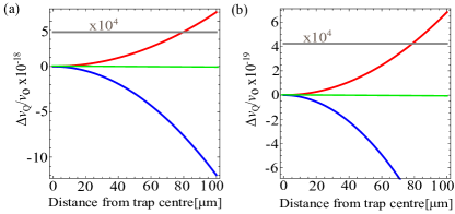
Figure 4: (Color online) Spatial dependence of the fractional electric quadrupole shifts $\Delta\nu_{Q}/\nu_{o}$ for the E2 and E3-clock transitions of $\rm{{}^{171}Yb^{+}}$. The quadrupole trapping potential produces a constant shift (gray). The spatial dependency in the shift along the radial (red) and axial (blue) directions arise from the anharmonic components $k>2$ of $\Phi^{(k)}$.

Due to its residual thermal motion of the ion after the laser cooling, it is unlikely to probe the clock transition while the ion is sitting at the center of the trap. Also there is a possibility that the mean position of the ion is few 10 $\mu$m away from the trap center due to imperfect stray field compensation. This results to a spatially dependent $\Delta\nu_{Q}$ in a non-ideal ion trap. At any position, the shift due to potentials for $k>2$ increases following a power law of order $k-2$ to the separation of the ion from the trap center, as shown in Fig. 2 (a, b) for our optimized trap geometry. Figure 4 shows spatial variation of $\Delta\nu_{Q}/\nu_{0}$ due to $\Phi^{(4)}$ and compares that with shift resulting from $\Phi^{(2)}$. The shift due to $\Phi^{(4)}$ is found to be four orders of magnitude smaller in our particular trap design than the contribution due to $\Phi^{(2)}$. However, our analysis shows that a wrong choice of the trap electrode geometry could easily increase $\Delta\nu_{Q}$ resulting from $\Phi^{(4)}$ by few orders of magnitude. The quadrupole shift due to $\Phi^{(2)}$ can be eliminated by measuring the clock frequency along the three mutually orthogonal orientations in the lab frame while quantizing the ion using the magnetic fields of equal amplitudes Itano_Nist_2000 ; Berkeland_JAP_1998 . In Fig. 4, we show such an angular averaging can eliminate the quadrupole shift resulting from $\Phi^{(4)}$ provided the trap assembly is perfectly axially symmetric. In practice the trap can deviate from such an ideal situation which could lead to inaccuracy in eliminating the quadrupole shift by angular averaging. In such a non ideal trap the inaccuracies of eliminating the quadrupole shift are generally induced by $\Phi^{(4)}$. Thus the present analysis also helps us in understanding to build a suitable trap electrode design where the effect of $\Phi^{(4)}$ in the quadrupole shift can be reduced.

The formula for evaluating the quadrupole shift given by

$$\Delta\nu_{Q}=\frac{c_{2}U}{R^{2}}\times\mathcal{F}_{Q}\times\Theta.$$ (31)

Substituting values of $\Theta$s from Table 1, we estimate these shifts for a constant $c_{2}U/R^{2}=932$ V/cm² which is expected in our trap geometry at $U=10$ V. All the resultant quadrupole shifts for the E2 and E3-clock transitions are shown in Figs. 5 (a) and (b), respectively. This shows that in our trap we will be able to measure the quadrupole moment of the $5d~{}^{2}D_{3/2}(F=2)$ state an accuracy of 1 part in $10^{3}$. This uncertainty will be one order of magnitude better than the previous measurement Schneider_PRL_2005 . Similarly, the quadrupole moment of the $4f^{13}6s^{2}~{}^{2}F_{7/2}(F=3)$ state was previously measured with $~{}12\%$ accuracy. We are also expecting to improve accuracy of this quantity using our proposed ion trap. This will help to verify the reported discrepancies among the experimental and theoretical results.

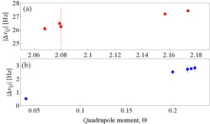
Figure 5: (Color online) The electric quadrupole shifts due to the previously reported works and estimated values from this work are shown in (a) for the $6s~{}{{}^{2}}S_{1/2}\rightarrow 5d~{}{{}^{2}}D_{3/2}$ and (b) for the $6s~{}{{}^{2}}S_{1/2}\rightarrow 4f^{13}6s^{2}~{}{{}^{2}}F_{7/2}$ clock transitions.

V Conclusion

We have proposed a suitable ion trap geometry for carrying out accurate measurements of the quadrupole shifts of the $6s~{}{{}^{2}}S_{1/2}\rightarrow 5d~{}{{}^{2}}D_{3/2}$ and $6s~{}{{}^{2}}S_{1/2}\rightarrow 4f^{13}6s^{2}~{}{{}^{2}}F_{7/2}$ clock transitions in the ¹⁷¹Yb⁺. We have also carried out calculation of $\Theta$ values of the $5d^{2}D_{3/2}$ and $4f^{13}6s^{2}~{}{{}^{2}}F_{7/2}$ states of ¹⁷¹Yb⁺ using the RCC method that are used in our analysis. We have identified an end cap ion trap geometry which can produce nearly ideal harmonic confinement to minimize the electric quadrupole shift. We also showed that a wrong choice of the ion trap geometry would increase the quadrupole shift resulting from $\Phi^{(4)}$ by two orders magnitude higher than our optimized geometry. To get a figure of merit we have estimated the quadrupole shifts along with their uncertainties in our proposed setup and compared the result with the previously available values. In our optimized ion trap we are expecting to measure the quadrupole moment of the $5d^{2}D_{3/2}$ state with an accuracy one part in $10^{3}$. We are also aiming to measure the quadrupole moment of the $4f^{13}6s^{2}~{}{{}^{2}}F_{7/2}$ state reliably that could possibly explain the discrepancy between the experimental and theoretical results.

References

- (1) A. Bauch, and H. R. Telle, Rep. Prog. Phys. 65, 789 (2002).
- (2) N. Poli, C. W. Oates, P. Gill, and G. M. Tino, Riv. Nuovo Cimento 36, 555 (2013).
- (3) M. Takamoto, I. Ushijima, M. Das, N. Nemitz, T. Ohkubo, K. Yamanaka, N. Ohmae, T. Takano, T. Akatsuka, A. Yamaguchi, and H. Katori, C. R. Phys. 16, 489 (2015).
- (4) T. Rosenband et. al., Science 319, 1808 (2008).
- (5) P. Gill, G. P. Barwood, H. A. Klein, G. Huang, S. A. Webster, P. J. Blythe, K. Hosaka, S. N. Lea and H. S. Margolis, IEEE Meas. Sci. Technol. 14, 1174-1186 (2003).
- (6) R. M. Godun et. al., Phys. Rev. Lett. 113, 210801 (2014).
- (7) C. Tamm, S. Weyers, B. Lipphardt, and E. Peik, Phys. Rev. A 80, 043403 (2009).
- (8) N. Huntemann, M. Okhapkin, B. Lipphardt, S. Weyers, Chr. Tamm, and E. Peik, Phys. Rev. Lett. 108, 090801 (2012).
- (9) N. Huntemann, B. Lipphardt, Chr. Tamm, V. Gerginov, S. Weyers, and E. Peik, Phys. Rev. Lett. 113, 210802 (2014).
- (10) Y. H. Wang, R. Dumke, T. Liu, A. Stejskal, Y. N. Zhao, J. Zhang, Z. H. Lu, L. J. Wang, Th. Becker, H. O. Walther, Opt. Comm. 273, 526 (2007).
- (11) P. Dubé, Alan A. Madej, Zichao Zhou, and John E. Bernard, Phys. Rev. A 87 023806 (2013).
- (12) G. P. Barwood, G. Huang, H. A. Klein, L. A. M. Johnson, S. A. King, H. S. Margolis, K. Szymaniec, and P. Gill, Phys. Rev. A 89, 050501(R) (2014).
- (13) Y. Huang, P. Liu, W. Bian, H. Guan, K. Gao, Applied Physics B 114, 189 (2014).
- (14) M. Kajita, Y. Li, K. Matsubara, K. Hayasaka and M. Hosokawa, Phys. Rev. A 72, 043404 (2005).
- (15) C. W. Chou, D. B. Hume, J. C. J. Koelemeij, D. J. Wineland, and T. Rosenband, Phys. Rev. Lett. 104, 070802 (2010).
- (16) D. K. Nandy and B. K. Sahoo, Phys. Rev. A 90, 050503(R) (2014).
- (17) S. Webster, R. Godun, S. King, G. Huang, B. Walton, V. Tsatourian,, H. Margolis, S. Lea and P. Gill, IEEE Trans. on Ultrasonics, Ferroelectrics, and Frequency Control 57, 3 (2010).
- (18) C. Tamm, N. Huntemann, B. Lipphardt, V. Gerginov, N. Nemitz, M. Kazda, S. Weyers, and E. Peik, Phys. Rev. A 89, 023820 (2014).
- (19) M. Roberts, P. Taylor, S. V. Gateva-Kostova, R. B. M. Clarke, W. R. C. Rowley and P. Gill Phys. Rev. A 60, 4 (1999).
- (20) S. A. King, New J. Phys. 14, 013045 (2012).
- (21) V. A. Dzuba and V. V. Flambaum, Phys. Rev. A 83, 052513 (2011).
- (22) B. K. Sahoo and B. P. Das, Phys. Rev. A 84, 010502(R) (2011).
- (23) V. A. Dzuba, V. V. Flambaum, M. S. Safronova, S. G. Porsev, T. Pruttivarasin, M. A. Hohensee, H. Häffner, arXiv:1507.06048v1 (2015).
- (24) V. A. Dzuba, V. V. Flambaum, and M. V. Marchenko, Phys. Rev. A 68, 022506 (2003).
- (25) V. A. Dzuba and V. V. Flambaum, Phys. Rev. A 77, 012515 (2008).
- (26) P. B. R. Nisbet-Jones, S. A. King, J. M. Jones, R. M. Godun, C. F. A. Baynham, K. Bongs, M. Doleal, P. Balling, and P. Gill, arXiv:1510.06341v1.
- (27) T. Schneider, E. Peik, and Chr. Tamm., Phys. Rev. Lett. 94, 230801 (2005).
- (28) P. J. Blythe, S. A. Webster, K. Hosaka, and P. Gill, J. Phys. B 36, 981 (2003).
- (29) S. G. Porsev, M. S. Safronova and M. G. Kozlov, Phys. Rev. A 86, 022504 (2012).
- (30) W. M. Itano, Phys. Rev. A 73, 022510 (2006).
- (31) K. V. P. Latha et al. Phys. Rev. A 76, 062508 (2007).
- (32) A. Rastogi, N. Batra, A. Roy, J. Thangjam, V. P. S. Kalsi, S. Panja, and S. De, MAPAN-J. of Metrology Society of India 30, 169 (2015).
- (33) S. De, N. Batra, S. Chakrabory , S. Panja and A. Sengupta, Current Science 106, 1348 (2014).
- (34) N. F. Ramsey Molecular Beams, (Oxford Univ. Press, London, 1956).
- (35) A. R. Edmonds Angular Momentum in Quantum Mechanics, (Princeton Univ. Press, New Jersey, 1974).
- (36) I. Lindgren and J. Morrison, Atomic Many-Body Theory, Second Edition, (Springer-Verlag, Berlin, Germany 1986).
- (37) D. K. Nandy and B. K. Sahoo, Phys. Rev. A 88, 052512 (2013).
- (38) B. K. Sahoo, D. K. Nandy, B. P. Das, and Y. Sakemi, Phys. Rev. A 91, 042507 (2015).
- (39) Y. Singh and B. K. Sahoo, Phys. Rev. A 91, 030501(R) (2015).
- (40) W. Paul, Rev. of Mod. Phys. 62, 531 (1990).
- (41) C. A. Schrama, E. Peik, W. W. Smith and H. Walther, Opt. Com. 101, 32 (1993).
- (42) B. Stein, Ph.D. thesis, University of Hannover (2010).
- (43) M. Dolez̆al, P. Balling, P. B. R. Nisbet-Jones, S. A. King, J. M. Jones, H A Klein, P. Gill, T. Lindvall, A. E. Wallin, M. Merimaa, C. Tamm, C. Sanner, N. Huntemann, N. Scharnhorst, I. D. Leroux, P. O. Schmidt, T. Burgermeister, T. E. Mehlst ubler, and E. Peik, arXiv:1510.05556 (2015).
- (44) F. G. Major, V. N. Gheorghe and G. Werth Charged Particle Traps, (Springer, New York, 2010).
- (45) 3D Charged Particle Optics program (CPO-3D) CPO Ltd., USA.
- (46) D. J. Berkeland, J. D. Miller, J. C. Bergquist, W. M. Itano, and D. J. Wineland, J. Appl. Phys. 83, 10 (1998).
- (47) J. Keller, H. L. Partner, T. Burgermeister, and T. E. Mehlstubler arXiv:1505.05907v1 (2015).
- (48) The ion trap geometry dependent dynamics have been studied, N. Batra, S. De., and S. Panja, [Manuscript in preperation].
- (49) W. M. Itano, J. Res. Nat. Inst. Stand. Tech., USA 105, 829 (2000).