Leading gradient correction to the kinetic energy for two-dimensional fermion gases

Abstract

Density functional theory (DFT) is notorious for the absence of gradient corrections to the two-dimensional (2D) Thomas-Fermi kinetic-energy functional; it is widely accepted that the 2D analog of the 3D von Weizsäcker correction vanishes, together with all higher-order corrections. Contrary to this long-held belief, we show that the leading correction to the kinetic energy does not vanish, is unambiguous, and contributes perturbatively to the total energy. This insight emerges naturally in a simple extension of standard DFT, which has the effective potential energy as a functional variable on equal footing with the single-particle density.

Introduction Recent advances in the experimental creation and control of ultracold Fermi gases Giorgini+2:08 in two-dimensional (2D) geometries Martiyanov2010 ; Dyke2011 ; Makhalov2014 ; Ries2015 ; Fenech2016 ; Boettcher2016 have triggered theoretical work on the semiclassical description of fermionic atoms by density functional theory (DFT) Fang+1:11 ; vanZyl+2:13 ; vanZyl2014 ; vanZyl2015 . While the Thomas-Fermi (TF) approximation to the kinetic-energy functional is accurate enough at the early stage of these investigations, better approximations will eventually be required for, say, more precise thermometry Stewart2006 ; Lu2012 ; Aikawa+5:14 and more realistic descriptions of interfaces in multi-component Fermi gases Partridge2006 ; Du2008 ; Ketterle2009 ; Conduit+1:09 ; Zwierlein2011 ; Sanner+5:12 ; TrGrBrRz2015 . The DFT formalism of Kohn-Sham (KS) type handles the kinetic-energy contribution accurately, but at the price of a large overhead of single-particle orbitals Karlicky2012 ; Rasmussen2015 ; Hu2015 . Whereas highly precise KS calculations are standard fare in 3D chemical physics and material science, the problematic dimensional reduction to 2D requires tailored approximations of the exchange-correlation functional, for which no general consensus has been reached Constantin2008 ; Raesaenen2010b ; Chiodo2012 . Generally, significant efforts are spent on improving orbital-free approximations of functionals, not only within the KS scheme Perdew2006 ; Lee2009 ; Sun2012 ; Sun2013 , and particularly in 2D Jiang2004 ; Pittalis2009 ; Raesaenen2010 , but foremost because an accurate orbital-free DFT would excel by superior computational efficiency Cangi2011 ; Burke2012 ; Karasiev2013 ; Burke2015 .

Improving upon the TF kinetic energy functional requires gradient terms that account for the inhomogeneity in the single-particle density to leading order. Unfortunately, at first sight it appears that the 2D analog of the 3D von Weizsäcker (vW) correction has a vanishing coefficient, and that all higher-order corrections vanish, too. This has been known for decades, at least since the early 1990s Holas+2:91 ; Shao:93 , and has become generally accepted wisdom (see, for example, Brack+1:03 ; Koivisto+1:07 ; Putaja+4:12 ). We are thus confronted with a dilemma: On the one hand, we know that the TF approximation cannot be exact; on the other hand, there is no established pathway toward nonzero corrections. It is understandable, then, that various ad-hoc corrections have been invented, such as the vW-type term vanZyl+2:13 and the nonlocal average-density functional recently proposed by van Zyl et al. vanZyl2014 ; vanZyl2015 .

However, systematic progress is possible without improvisation. In this Letter, we provide an analytical, orbital-free approach to the calculation of the leading gradient correction to the TF kinetic-energy functional. By a simple extension of standard DFT, which uses the effective potential energy as an independent variable on equal footing with the single-particle density Englert:92 , we obtain a nonzero gradient correction that is unambiguous and yields a first-order correction to the energy that can be evaluated by the usual perturbation-theory method. The problem with, and the ambiguities of, the gradient correction to the density functional arise when one eliminates the effective potential energy in order to arrive at a functional of the density alone.

Functionals We review briefly the construction of the joint functional of the single-particle density $n(\vecfont{r})$ and the effective potential energy $V(\vecfont{r})$, as given in Englert:92 . We incorporate the particle-count constraint

$$N=\int(\mathrm{d}\vecfont{r})\,n(\vecfont{r})$$ (1)

into the density functional

$$E[n]=E_{\mathrm{kin}}[n]+\int(\mathrm{d}\vecfont{r})\,V_{\mathrm{ext}}(\vecfont{r})n(\vecfont{r})+E_{\mathrm{int}}[n]$$ (2)

with the aid of a Lagrange multiplier, the chemical potential $\mu$,

$$E[n,\mu]=E[n]+\mu{\left(N-\int(\mathrm{d}\vecfont{r})\,n(\vecfont{r})\right)}\,.$$ (3)

Here $(\mathrm{d}\vecfont{r})$ denotes the volume element at position $\vecfont{r}$; $V_{\mathrm{ext}}(\vecfont{r})$ is the external potential energy for a probe particle at $\vecfont{r}$; $N$ is the total number of particles; $E_{\mathrm{kin}}[n]$ is the density functional of the kinetic energy; and $E_{\mathrm{int}}[n]$ is that of the particle-particle interaction energy. The response of $E_{\mathrm{kin}}[n]$ to variations of the density identifies the effective potential energy $V(\vecfont{r})$,

$$\delta E_{\mathrm{kin}}[n]=-\int(\mathrm{d}\vecfont{r})\,\delta n(\vecfont{r})[V(\vecfont{r})-\mu]\,,$$ (4)

and the Legendre transformation

$$E_{1}[V-\mu]=E_{\mathrm{kin}}[n]+\int(\mathrm{d}\vecfont{r})\,[V(\vecfont{r})-\mu]n(\vecfont{r})$$ (5)

introduces the potential-energy functional $E_{1}[V-\mu]$, since

$$\delta E_{1}[V-\mu]=\int(\mathrm{d}\vecfont{r})\,\delta[V(\vecfont{r})-\mu]\,n(\vecfont{r})$$ (6)

has no contribution associated with $\delta n(\vecfont{r})$. Accordingly, we have the joint functional

$$E[V,n,\mu] = E_{1}[V-\mu]-\int(\mathrm{d}\vecfont{r})\,[V(\vecfont{r})-V_{\mathrm{ext}}(\vecfont{r})]n(\vecfont{r})$$ (7)

$$\mbox{}+E_{\mathrm{int}}[n]+\mu N\,,$$

which is stationary at the actual $V(\vecfont{r})$, $n(\vecfont{r})$, and $\mu$.

The structure of Eq. (5) shows that ${E_{1}[V-\mu]}$ is the expectation value of

$$\sum_{k=1}^{N}[T(\vecfont{P}_{k})+V(\vecfont{R}_{k})-\mu]=\sum_{k=1}^{N}[H(\vecfont{R}_{k},\vecfont{P}_{k})-\mu]\,,$$ (8)

the Hamiltonian of noninteracting particles with kinetic energy $T(\vecfont{p})$ and potential energy ${V(\vecfont{r})-\mu}$ for each particle, in the $N$-particle ground state of the physical Hamiltonian

$$\sum_{k=1}^{N}[T(\vecfont{P}_{k})+V_{\mathrm{ext}}(\vecfont{R}_{k})]+H_{\mathrm{int}}$$ (9)

that involves the potential energy $V_{\mathrm{ext}}(\vecfont{r})$ of the external forces and the full $N$-particle interaction Hamiltonian $H_{\mathrm{int}}$ rp-RP .

The vanishing linear response of $E[V,n,\mu]$ to variations $\delta V(\vecfont{r})$, $\delta n(\vecfont{r})$, and $\delta\mu$ implies the set of equations

$${\delta V:} n(\vecfont{r}) = \frac{\delta}{\delta V(\vecfont{r})}E_{1}[V-\mu]\,,$$ (10a)

$${\delta n:} V(\vecfont{r}) = V_{\mathrm{ext}}(\vecfont{r})+\frac{\delta}{\delta n(\vecfont{r})}E_{\mathrm{int}}[n]\,,$$ (10b)

$${\delta\mu:} N = -\frac{\partial}{\partial\mu}E_{1}[V-\mu]\,,$$ (10c)

jointly solved by the actual effective potential energy $V(\vecfont{r})$, the actual single-particle density $n(\vecfont{r})$, and the actual value of the chemical potential $\mu$. Equation (1) is recovered by combining Eqs. (10a) and (10c). We can convert $E[V,n,\mu]$ into a functional $E[V,\mu]$ of $V(\vecfont{r})$ and $\mu$ by solving Eq. (10b) for $n(\vecfont{r})$ in terms of $V(\vecfont{r})$. Likewise, we return from $E[V,n,\mu]$ to $E[n,\mu]$ by solving Eq. (10a) for $V(\vecfont{r})$ in terms of $n(\vecfont{r})$ and using this $V(\vecfont{r})$ in $E[V,n,\mu]$. In particular, the kinetic-energy density functional is obtained as

$$E_{\mathrm{kin}}[n]=\biggl{(}\!E_{1}[V-\mu]-\!\int(\mathrm{d}\vecfont{r})\,[V(\vecfont{r})-\mu]n(\vecfont{r})\!\biggr{)}\Biggr{|}_{\mbox{\footnotesize{$\begin{array}[t]{l}V(\vecfont{r})-\mu\\ \mbox{from \eqref{eq:A10a}}\end{array}$}}}$$ (11)

provided that we can carry out the necessary steps. For the familiar TF model for the 3D electron gas in atoms, these matters are discussed in Englert:88 .

As an example in 2D, we consider a gas of $N$ unpolarized spin-$\frac{1}{2}$ atoms of mass $m$ with a repulsive contact interaction of strength $W>0$. We have

$$E[V,n,\mu] = -\frac{m}{2\pi\hbar^{2}}\int(\mathrm{d}\vecfont{r})\,[\mu-V(\vecfont{r})]_{+}^{2}$$ (12)

$$\mbox{}-\int(\mathrm{d}\vecfont{r})\,[V(\vecfont{r})-V_{\mathrm{ext}}(\vecfont{r})]n(\vecfont{r})$$

$$\mbox{}+\frac{W}{2}\int(\mathrm{d}\vecfont{r})\,n(\vecfont{r})^{2}+\mu N$$

in TF approximation, where $\vecfont{r}$ is now a 2D position vector and $(\mathrm{d}\vecfont{r})$ is its area element, and $[x]_{+}$ selects the positive values of variable $x$, that is: $[x]_{+}=x\eta(x)$, with Heaviside’s unit step function $\eta(\ )$. The actual $V(\vecfont{r})$, $n(\vecfont{r})$, and $\mu$ solve

$$n(\vecfont{r}) = \frac{m}{\pi\hbar^{2}}[\mu-V(\vecfont{r})]_{+}\,,$$ (13a)

$$V(\vecfont{r}) = V_{\mathrm{ext}}(\vecfont{r})+Wn(\vecfont{r})\,,$$ (13b)

resulting in $n(\vecfont{r})=(W+\pi\hbar^{2}/m)^{-1}[\mu-V_{\mathrm{ext}}(\vecfont{r})]_{+}$ for the density, with the value of $\mu$ determined by Eq. (1), and the effective potential energy then from Eq. (13b).

The kinetic-energy functional

$$E_{\mathrm{kin}}[n]=\frac{\pi\hbar^{2}}{2m}\int(\mathrm{d}\vecfont{r})\,n(\vecfont{r})^{2}$$ (14)

is obtained in accordance with Eq. (11), and we note that solving Eq. (13a) for ${V(\vecfont{r})-\mu}$ in terms of $n(\vecfont{r})$ is only possible where ${n(\vecfont{r})>0}$, whereas this equation does not tell us the value of $V(\vecfont{r})$ where the density vanishes. This is of no consequence in this example, but the proviso at Eq. (11) must be kept in mind.

The reduced functionals

$$E[n]=\frac{\pi\hbar^{2}+mW}{2m}\int(\mathrm{d}\vecfont{r})\,n(\vecfont{r})^{2}+\int(\mathrm{d}\vecfont{r})\,V_{\mathrm{ext}}(\vecfont{r})n(\vecfont{r})$$ (15)

and

$$E[V,\mu] = -\frac{m}{2\pi\hbar^{2}}\int(\mathrm{d}\vecfont{r})\,[\mu-V(\vecfont{r})]_{+}^{2}$$

$$\mbox{}-\frac{1}{2W}\int(\mathrm{d}\vecfont{r})\,[V(\vecfont{r})-V_{\mathrm{ext}}(\vecfont{r})]_{+}^{2}+\mu N$$

are clearly quite different, they are not just reparameterizations of each other. The density functional $E[n]$ is minimal for the actual density whereas the potential-energy functional is maximal for the actual potential energy and the actual value of the chemical potential,

$$E(N)=\min_{n}\{E[n]\}=\max_{V,\mu}\{E[V,\mu]\}\,,$$ (17)

where the permissible densities obey the constraint of Eq. (1). We get upper bounds on the actual energy $E(N)$ from trial densities in $E[n]$, and lower bounds from trial values for $V(\vecfont{r})$ and $\mu$ in $E[V,\mu]$.

We must note in this context that the potential functionals of Cangi+2:13 are not of the $E[V,\mu]$ kind. Rather, they are density functionals of the usual $E[n]$ kind in disguise, with the density parameterized in terms of the external potential (as one does at an intermediate step in the standard proof of the Hohenberg-Kohn theorem). Since $E[n]$ provides upper bounds on the actual energy, so do these functionals of the $E\bigl{[}n[V_{\mathrm{ext}}]\bigr{]}$ type.

Gradient corrections The Hamiltonian in Eq. (8) is that of noninteracting particles, with the kinetic energy $T(\vecfont{p})=\vecfont{p}^{2}/(2m)$ fixed and different choices for $V(\vecfont{r})-\mu$. Since there is one copy of the single-particle Hamiltonian $H(\vecfont{R},\vecfont{P})$ for each particle, it follows that $E_{1}[V-\mu]$ is the trace of some function $f(H-\mu)$ of $H(\vecfont{R},\vecfont{P})-\mu$ Englert:92 . For truly noninteracting fermions, all single-particle orbitals with energies below the chemical potential would be occupied and none above, so that ${f(x)=x\eta(-x)=-[-x]_{+}}$ then. For interacting fermions, this $f(x)$ is an approximation, but it is sufficiently accurate for the current purpose, and so we approximate $E_{1}[V-\mu]$ by

$$E_{1}[V-\mu] = -\textnormal{tr}{\left\{\bigl{[}\mu-H(\vecfont{R},\vecfont{P})\bigr{]}_{+}\right\}}$$ (18)

$$= -2\int\!\frac{(\mathrm{d}\vecfont{r})(\mathrm{d}\vecfont{p})}{(2\pi\hbar)^{2}}\Bigl{(}[\mu-H\bigr{]}_{+}\Bigr{)}_{\textsc{w}}(\vecfont{r},\vecfont{p})\,,\qquad$$

where we exhibit a factor of two for the spin multiplicity and evaluate the quantum-mechanical trace by the phase-space integral of the Wigner function for the single-particle operator $[\mu-H(\vecfont{R},\vecfont{P})]_{+}$.

The lowest-order terms in a gradient expansion of the Wigner function $[g(A)]_{\textsc{w}}$ of an operator function $g(A)$ in terms of the Wigner function $A_{\textsc{w}}$ of the argument are Wigner-lead-corr

$$[g(A)]_{\textsc{w}} = g(A_{\textsc{w}})-\frac{\hbar^{2}}{16}\bigl{\{}A_{\textsc{w}}\Lambda^{2}A_{\textsc{w}}\bigr{\}}g^{\prime\prime}(A_{\textsc{w}})$$ (19)

$$\mbox{}+\frac{\hbar^{2}}{24}\bigl{\{}A_{\textsc{w}}\Lambda A_{\textsc{w}}\Lambda A_{\textsc{w}}\bigr{\}}g^{\prime\prime\prime}(A_{\textsc{w}})\,,$$

where ${\Lambda=\loarrow{\partial_{\vecfont{r}}}\cdot\roarrow{\partial_{\vecfont{p}}}-\loarrow{\partial_{\vecfont{p}}}\cdot\roarrow{\partial_{\vecfont{r}}}}$ is the two-sided differential operator of the classical Poisson bracket, which acts only on the $A_{\textsc{w}}$ factors standing right next to it inside the curly brackets, and terms of order $(\hbar\Lambda)^{4}$ and higher are neglected in Eq. (19). For ${A=H(\vecfont{R},\vecfont{P})-\mu}$ with ${A_{\textsc{w}}=H(\vecfont{r},\vecfont{p})-\mu}$ and ${g(x)=[-x]_{+}}$ with the derivatives ${g^{\prime\prime}(x)=\delta(x)}$ and ${g^{\prime\prime\prime}(x)=\delta^{\prime}(x)}$, we find

$$E_{1}[V-\mu] = -\frac{m}{2\pi\hbar^{2}}\int(\mathrm{d}\vecfont{r})\,[\mu-V(\vecfont{r})]_{+}^{2}$$ (20)

$$\mbox{}+\frac{1}{24\pi}\int(\mathrm{d}\vecfont{r})\,\delta\bigl{(}\mu-V(\vecfont{r})\bigr{)}\bigl{[}\boldsymbol{\nabla}V(\vecfont{r})\bigr{]}^{2}.\qquad$$

The first term is the TF approximation that was already used in Eq. (12), and the second term — of second order in the gradient — is the leading quantum correction, formally of relative size $\propto\hbar^{2}$. The resulting quantum correction to the TF energy is obtained by a perturbative evaluation,

$$\Delta_{\mathrm{qu}}E=\frac{1}{24\pi}\int(\mathrm{d}\vecfont{r})\,\delta(\mu-V_{\textsc{tf}})(\boldsymbol{\nabla}V_{\textsc{tf}})^{2}\,,$$ (21)

with the effective potential energy $V_{\textsc{tf}}(\vecfont{r})$ found in the TF approximation that neglects the second term in Eq. (20). Exceptional cases aside, the gradient of $V_{\textsc{tf}}$ is continuous at the border between the classically allowed and forbidden regions selected by the delta function, and there is no ambiguity in evaluating the integral ourEX .

In view of Eq. (11), this $\Delta_{\mathrm{qu}}E$ is also the quantum correction that the leading correction to the TF approximation of $E_{\mathrm{kin}}[n]$ in Eq. (14) should produce. We find this corresponding gradient correction by solving

$$n=\frac{m}{\pi\hbar^{2}}[\mu-V]_{+}+\frac{1}{24\pi}\bigl{[}\boldsymbol{\nabla}^{2}\eta(\mu-V)+\delta(\mu-V)\boldsymbol{\nabla}^{2}(\mu-V)\bigr{]}$$ (22)

for $\mu-V$ in terms of $n$ up to second order in the gradient,

$$\mu-V=\frac{\pi\hbar^{2}}{m}{\left[n-\frac{1}{24\pi}\boldsymbol{\nabla}^{2}\eta(n)-\frac{1}{24\pi}\delta(n)\boldsymbol{\nabla}^{2}n\right]}\,,$$ (23)

and then using this in Eq. (11) to arrive at

$$E_{\mathrm{kin}}[n]=\frac{\pi\hbar^{2}}{2m}\int(\mathrm{d}\vecfont{r})\,{\left[n(\vecfont{r})^{2}+\frac{1}{12\pi}\delta\bigl{(}n(\vecfont{r})\bigr{)}\bigl{(}\boldsymbol{\nabla}n(\vecfont{r})\bigr{)}^{2}\right]}\,.$$ (24)

The correction term ${\propto\delta(n)(\boldsymbol{\nabla}n)^{2}}$ is well known vW , but not universally established. It has been found by some methods used for deriving gradient corrections KKvsW (see, for example, Brack+1:03 ; vanZyl:00 ) or not found by other methods (see, for example, Holas+2:91 ; Shao:93 ; Koivisto+1:07 ; Putaja+4:12 ). When the term was found, it was discarded on the basis that it gives “a vanishing contribution to the integrated kinetic energy for physical densities which decay smoothly to zero as $r$ tends to infinity” vanZyl+2:13 , which is a reasonable argument.

In any case, the correction term is rather problematic. Recalling the remark after Eq. (14), we observe that Eq. (23) is restricted to regions where ${n(\vecfont{r})>0}$, and there we have ${\delta(n)=0}$. But what about the border region that solely contributes to $\Delta_{\mathrm{qu}}E$ in Eq. (21)? Further, an attempt at a perturbative evaluation,

$$\Delta_{\mathrm{qu}}E=\frac{\hbar^{2}}{24m}\int(\mathrm{d}\vecfont{r})\,\delta(n_{\textsc{tf}})(\boldsymbol{\nabla}n_{\textsc{tf}})^{2}\,,$$ (25)

requires the assignment of a value to $(\boldsymbol{\nabla}n_{\textsc{tf}})^{2}$ where the gradient of $n_{\textsc{tf}}$ is discontinuous. This is in marked contrast to $\Delta_{\mathrm{qu}}E$ in Eq. (21) where $\boldsymbol{\nabla}V_{\textsc{tf}}$ is (usually) continuous across the border between the classically allowed region ($\mu>V$) and the classically forbidden region ($\mu<V$).

Clearly, these problems occur in the transition from $E[V,n,\mu]$ to $E[n,\mu]$ and, eventually, to $E[n]$. We can stay out of trouble by consistently working with the joint functional $E[V,n,\mu]$. Also in other contexts, functionals of the effective potential energy have been more useful than the standard functionals of DFT V-func .

Not only the correction term ${\propto\delta(n)(\boldsymbol{\nabla}n)^{2}}$ has been found before, also intermediate equations such as Eq. (22) or similar appear in other derivations — with a colossal difference in physical meaning, however: The effective potential energy $V(\vecfont{r})$ is a variable of the functional $E[V,n,\mu]$ on equal footing with the density $n(\vecfont{r})$ and we prefer to keep $V$ in the formalism, rather than eliminating it. In other derivations, an auxiliary variable $V(\vecfont{r})$ is introduced as a technical tool for deriving statements about systems of noninteracting particles, is eliminated at the earliest convenience without a trace, and is never a variable of a functional. It is also worth remembering that the effective potential energy accounts for the interaction fully [see Eq. (10b)], and the functional $E_{1}[V-\mu]$, be it in TF approximation or beyond, is equally valid for interacting and noninteracting particles.

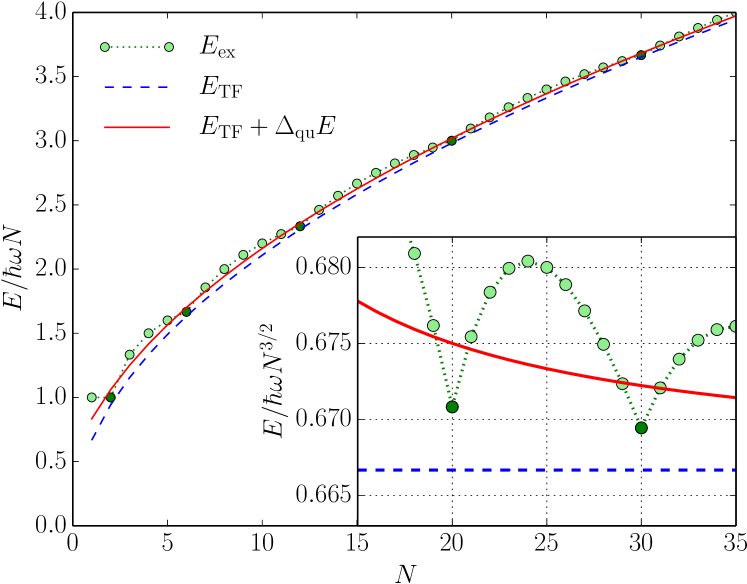
Figure 1: Energy of $N$ noninteracting fermions in an isotropic 2D harmonic trap with angular frequency $\omega$. Main plot: energy per particle. Inset: Zoom on the energy divided by the TF scaling $N^{3/2}$. Circles connected by dotted lines are the exact energies HarmOscEnergy ; dark circles denote the closed-shell values ${N=2,6,12,20,30}$. The dashed blue line is the TF approximation, Eq. (28), consistently below the exact energies. The full red line includes the leading quantum correction Eq. (29), interpolating the oscillations of the exact values above the TF result.

2D harmonic oscillator The external harmonic-oscillator potential ${V_{\mathrm{ext}}(\vecfont{r})=\frac{1}{2}m\omega^{2}\vecfont{r}^{2}}$ is omnipresent in trapped 2D Fermi gases Stanescu2007 ; Martiyanov2010 ; Dyke2011 ; Makhalov2014 ; Ries2015 ; Fenech2016 ; Boettcher2016 and often appropriate for other systems, like electrons in quantum dots Reimann2002 . It is good practice to employ exactly solvable models for judging the accuracy of approximate energy functionals as done in Holas+2:91 ; Brack2001 ; vanZyl+2:13 for harmonically confined noninteracting particles KSvsSemiclassics . We follow this tradition and examine $E[V,n,\mu]$ in TF approximation,

$$E[V,n,\mu] = -\frac{m}{2\pi\hbar^{2}}\int(\mathrm{d}\vecfont{r})\,[\mu-V(\vecfont{r})]_{+}^{2}$$

$$\mbox{}-\int(\mathrm{d}\vecfont{r})\,\Bigl{[}V(\vecfont{r})-\frac{1}{2}m\omega^{2}\vecfont{r}^{2}\Bigr{]}n(\vecfont{r})+\mu N\,.$$

The stationary values are $V_{\textsc{tf}}(\vecfont{r})=V_{\mathrm{ext}}(\vecfont{r})=\frac{1}{2}m\omega^{2}\vecfont{r}^{2}$, of course, as well as

$$n_{\textsc{tf}}(\vecfont{r})=\frac{m\omega}{\pi\hbar}\Bigl{[}N^{\frac{1}{2}}-\frac{m\omega}{2\hbar}\vecfont{r}^{2}\Bigr{]}_{+}\quad\mbox{and}\quad\mu_{\textsc{tf}}=\hbar\omega N^{\frac{1}{2}}\,.$$ (27)

They yield the TF energy

$$E_{\textsc{tf}}(N)=-\frac{1}{3}\hbar\omega N^{\frac{3}{2}}+0+\hbar\omega N^{\frac{3}{2}}=\frac{2}{3}\hbar\omega N^{\frac{3}{2}}\,,$$ (28)

where the three-term sum refers to the three contributions in Eq. (Leading gradient correction to the kinetic energy for two-dimensional fermion gases). The quantum correction of Eq. (21) is

$$\Delta_{\mathrm{qu}}E(N)=\frac{1}{6}\hbar\omega N^{\frac{1}{2}}\,,$$ (29)

which is unambiguous, definitely nonzero, and small compared with the leading TF contribution. Figure 1 shows that $\Delta_{\mathrm{qu}}E(N)$ gives an average account of the oscillatory difference between the exact energy HarmOscEnergy and the TF approximation.

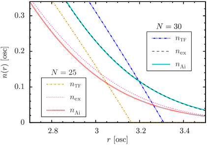
Figure 2: Densities $n(r)$ of noninteracting spin-$\frac{1}{2}$ particles in an external harmonic-oscillator potential in the vicinity of the border between the classically allowed and forbidden regions. The abscissa is the radial distance $r=|\vecfont{r}|$ in oscillator units. For five filled shells (${N=30}$) and for the fifth shell half-full (${N=25}$), the plot shows the exact densities $n_{\mathrm{ex}}^{\ }$, their TF approximations $n_{\textsc{tf}}^{\ }$, and the densities $n_{\mathrm{Ai}}^{\ }$ obtained with Airy-averaging techniques.

Particle density The leading gradient correction of Eq. (20) is fine for the perturbative evaluation as in Eq. (21) but the implied correction to the single-particle density in Eq. (22) is singular and entirely localized at the border between the classically allowed and forbidden regions. A fully satisfactory improvement over the TF approximation should yield a smooth transition across this border. This is achieved with the 2D analogs of the 3D Airy-averaging techniques Englert+1:84b ; Englert:88 , by which one obtains better approximations for $E_{1}[V-\mu]$ and the resulting density Airy-av . These matters and others will be discussed elsewhere Trappe+4:IP . Here we are content with showing, in Fig. 2, two such densities for the harmonic-oscillator example above, together with the exact densities and their TF approximations. Clearly, the Airy averages improve matters much and yield very reasonable densities Alt-E1 .

Summary We established the leading gradient correction to the TF approximation for the kinetic energy for a 2D gas of fermions. This quantum correction is unambiguous and its nonzero contribution to the energy can be evaluated. These findings are at variance with traditional claims that the gradient corrections vanish in all orders. Having concluded that the derivations that support these claims are problematic in the transition from the joint density-potential functional to the density-only functional, we recommend working consistently with the joint functional.

Acknowledgments We thank P. Trevisanutto for valuable discussions. This work is funded by the Singapore Ministry of Education and the National Research Foundation of Singapore. H. K. N is also funded by a Yale-NUS College start-up grant. C. A. M. acknowledges the hospitality of Institut Non Linéaire de Nice (CNRS and Université de Nice) and Laboratoire de Physique Théorique (CNRS and UPS Toulouse).

References

- (1) S. Giorgini, L. P. Pitaevskii, and S. Stringari, Rev. Mod. Phys. 80, 1215 (2008).
- (2) K. Martiyanov, V. Makhalov, and A. Turlapov, Phys. Rev. Lett. 105, 030404 (2010).
- (3) P. Dyke, E. D. Kuhnle, S. Whitlock, H. Hu, M. Mark, S. Hoinka, M. Lingham, P. Hannaford, and C. J. Vale, Phys. Rev. Lett. 106, 105304 (2011).
- (4) V. Makhalov, K. Martiyanov, and A. Turlapov, Phys. Rev. Lett. 112, 045301 (2014).
- (5) M. G. Ries, A. N. Wenz, G. Zürn, L. Bayha, I. Boettcher, D. Kedar, P. A. Murthy, M. Neidig, T. Lompe, and S. Jochim, Phys. Rev. Lett. 114, 230401 (2015).
- (6) K. Fenech, P. Dyke, T. Peppler, M. G. Lingham, S. Hoinka, H. Hu, and C. J. Vale, Phys. Rev. Lett. 116, 045302 (2016).
- (7) I. Boettcher, L. Bayha, D. Kedar, P. A. Murthy, M. Neidig, M. G. Ries, A. N. Wenz, G. Zürn, S. Jochim, and T. Enss, Phys. Rev. Lett. 116, 045303 (2016).
- (8) B. Fang and B.-G. Englert, Phys. Rev. A83, 052517 (2011).
- (9) B. P. van Zyl, E. Zaremba, and P. Pisarski, Phys. Rev. A87, 043614 (2013).
- (10) B. P. van Zyl, A. Farrell, E. Zaremba, J. Towers, P. Pisarski, and D. A. W. Hutchinson, Phys. Rev. A89, 022503 (2014).
- (11) J. Towers, B. P. van Zyl, and W. Kirkby, Phys. Rev. B 92, 075129 (2015).
- (12) J. T. Stewart, J. P. Gaebler, C. A. Regal, and D. S. Jin, Phys. Rev. Lett. 97, 220406 (2006).
- (13) M. Lu, N. Q. Burdick, and B. L. Lev, Phys. Rev. Lett. 108, 215301 (2012).
- (14) K. Aikawa, A. Frisch, M. Mark, S. Baier, R. Grimm, and F. Ferlaino, Phys. Rev. Lett. 112, 010404 (2014).
- (15) G. B. Partridge, W. Li, R. I. Kamar, Y. A. Liao, and R. G. Hulet, Science 311, 503 (2006).
- (16) X. Du, L. Luo, B. Clancy, and J. E. Thomas, Phys. Rev. Lett. 101, 150401 (2008).
- (17) G.-B. Jo, Y.-R. Lee, J.-H. Choi, C. A. Christensen, T. H. Kim, J. H. Thywissen, D. E. Pritchard, and W. Ketterle, Science 325, 1521 (2009).
- (18) G. J. Conduit and B. D. Simons, Phys. Rev. Lett. 103, 200403 (2009).
- (19) A. Sommer, M. Ku, G. Roati, and M. W. Zwierlein, Nature 472, 201 (2011).
- (20) C. Sanner, E. J. Su, W. Huang, A. Keshet, J. Gillen, and W. Ketterle, Phys. Rev. Lett. 108, 240404 (2012).
- (21) M.-I. Trappe, P. Grochowski, M. Brewczyk, and K. Rzążewski, Phys. Rev. A93, 023612 (2016).
- (22) F. Karlický, R. Zbor̆il, and M. Otyepka, J. Chem. Phys. 137, 034709 (2012).
- (23) F. A. Rasmussen and K. S. Thygesen, J. Phys. Chem. C 119, 13169 (2015).
- (24) W. Hu, L. Lin, and C. Yang, J. Chem. Phys. 143, 124110 (2015).
- (25) L. A. Constantin, J. P. Perdew, and J. M. Pitarke, Phys. Rev. Lett. 101, 016406 (2008); Erratum: Phys. Rev. Lett. 101, 269902(E) (2008).
- (26) E. Räsänen, S. Pittalis, J. G. Vilhena, and M. A. L. Marques, Int. J. Quant. Chem. 110, 2308 (2010).
- (27) L. Chiodo, L. A. Constantin, E. Fabiano, and F. Della Sala, Phys. Rev. Lett. 108, 126402 (2012).
- (28) J. P. Perdew, L. A. Constantin, E. Sagvolden, and K. Burke, Phys. Rev. Lett. 97, 223002 (2006).
- (29) D. Lee, L. A. Constantin, J. P. Perdew, and K. Burke, J. Chem. Phys. 130, 034107 (2009).
- (30) J. Sun, B. Xiao, and A. Ruzsinszky, J. Chem. Phys. 137, 051101 (2012).
- (31) J. Sun, R. Haunschild, B. Xiao, I. W. Bulik, G. E. Scuseria, and J. P. Perdew, J. Chem. Phys. 138, 044113 (2013).
- (32) H. Jiang and W. Yang, J. Chem. Phys. 121, 2030 (2004).
- (33) S. Pittalis and E. Räsänen, Phys. Rev. B80, 165112 (2009).
- (34) E. Räsänen, S. Pittalis, and C. R. Proetto, Phys. Rev. B81, 195103 (2010).
- (35) A. Cangi, D. Lee, P. Elliott, K. Burke, and E. K. U. Gross, Phys. Rev. Lett. 106, 236404 (2011).
- (36) K. Burke, J. Chem. Phys. 136, 150901 (2012).
- (37) V. V. Karasiev, D. Chakraborty, O. A. Shukruto, and S. B. Trickey, Phys. Rev. B88, 161108(R) (2013).
- (38) A. Pribram-Jones, D. A. Gross, and K. Burke, Annu. Rev. Phys. Chem. 66, 283 (2015).
- (39) A. Holas, P. M. Kozlowski, and N. H. March, J. Phys. A: Math. Gen. 24, 4249 (1991).
- (40) J. Shao, Mod. Phys. Lett. B 7, 1193 (1993).
- (41) M. Brack and R. K. Bhaduri, Semiclassical Physics, Frontiers in Physics, Vol. 96 (Addison-Wesley, Reading, MA, 2003).
- (42) M. Koivisto and M. J. Stott, Phys. Rev. B76, 195103 (2007).
- (43) A. Putaja, E. Räsänen, R. van Leeuwen, J. G. Vilhena, and M. A. L. Marques, Phys. Rev. B85, 165101 (2012).
- (44) B.-G. Englert, Phys. Rev. A45, 127 (1992).
- (45) We use lower case letters , for the classical phase space variables and upper case letters , for the operators.
- (46) B.-G. Englert, Semiclassical Theory of Atoms, Lect. Notes Phys., Vol. 300 (Springer-Verlag, Berlin, 1988).
- (47) A. Cangi, E. K. U. Gross, and K. Burke, Phys. Rev. A88, 062505 (2013).
- (48) Wigner’s seminal work of 1932 Wigner:32 contains a particular case of Eq. (19), re-derived in many later papers; see, e.g., Grammaticos+1:79 . The general expression can be found in the appendix of Von-Eiff+1:91 .
-
(49)
The example of Eqs. (12)–(Leading gradient correction to the kinetic energy for two-dimensional
fermion gases) is a bit pathological in
this respect, but an easy cure is available:
Replace the contact interaction with an interaction that has a short
range ,
Solving the corresponding version of Eq. (13b) for is then accomplished by . With from Eq. (13a), this is a second-order differential equation for , and the resulting effective potential energy has a continuous gradient field.
- (50) The correction term differs in structure from the well-known vW correction to the kinetic energy functional in 3D, and the analogous 1D term (which, however, has a negative coefficient).
- (51) The Kirkwood and Kirzhnits (K&K) expansion methods are particularly popular. They are similar to, but different from, the Wigner-function based methods. In the K&K approaches, operator functions of and are ordered such that all s are to the left of all s in products (or vice versa), whereas a symmetric ordering underlies the Wigner-function methods.
- (52) B. P. van Zyl, Ph.D. thesis, Queen’s University, 2000; section 2.4.
- (53) There is, in particular, Schwinger’s derivation of the leading and second corrections to the TF energy of neutral atoms Schwinger:80 ; Schwinger:81 ; see also Englert:88 and references therein.
- (54) T. D. Stanescu, C. Zhang, and V. Galitski, Phys. Rev. Lett. 99, 110403 (2007).
- (55) S. M. Reimann and M. Manninen, Rev. Mod. Phys. 74, 1283 (2002).
- (56) M. Brack and B. P. van Zyl, Phys. Rev. Lett. 86, 1574 (2001).
- (57) For a meaningful comparison of the semiclassical approximation in Eq. (20) with the exact (KS) evaluation of the trace in Eq. (18), one should use the same effective potential energy in both expressions. Therefore, the use of noninteracting fermions is expedient in this context since the two self-consistent solutions of Eqs. (10) — one with the of Eq. (18), the other with that of Eq. (20) — yield different s if .
-
(58)
The exact energy is
where is the difference between and its nearest integer, with for closed shells.
- (59) B.-G. Englert and J. Schwinger, Phys. Rev. A29, 2339 (1984).
-
(60)
One main ingredient is the Airy-averaged version of Eq. (19),
where and is the Airy function. The right-hand side agrees with that of Eq. (19) to order and includes contributions from higher-order terms in a systematic way. It gives the exact for if the effective potential energy is that of a constant force.
- (61) M.-I. Trappe, Y. L. Len, H. K. Ng, C. A. Müller, and B.-G. Englert, in preparation.
- (62) If there are 2D and 3D analogs of the 1D densities of Ribeiro+4:15 , they offer another strategy for constructing improved approximations for .
- (63) E. Wigner, Phys. Rev. 40, 749 (1932).
- (64) B. Grammaticos and A. Voros, Ann. Phys. 123, 359 (1979).
- (65) D. Von-Eiff and M. K. Weigel, Z. Phys. A – Hadrons and Nuclei 339, 63 (1991).
- (66) J. Schwinger, Phys. Rev. A22, 1827 (1980).
- (67) J. Schwinger, Phys. Rev. A24, 2353 (1981).
- (68) R. F. Ribeiro, D. Lee, A. Cangi, P. Elliott, and K. Burke, Phys. Rev. Lett. 114, 050401 (2015).