Generalized canonical purification for density matrix minimization

Abstract

A Lagrangian formulation for the constrained search for the $N$-representable one-particle density matrix based on the McWeeny idempotency error minimization is proposed, which converges systematically to the ground state. A closed form of the canonical purification is derived for which no a posteriori adjustement on the trace of the density matrix is needed. The relationship with comparable methods are discussed, showing their possible generalization through the hole-particle duality. The appealing simplicity of this self-consistent recursion relation along with its low computational complexity could prove useful as an alternative to diagonalization in solving dense and sparse matrix eigenvalue problems.

As suggested 60 years agoMcWeeny (1956a); *McWeeny_density_1956b; *McWeeny_density_1957c, the idempotency property of the density matrix (DM) along with a minimization algorithm would be sufficient to solve for the electronic structure without relying on the time consuming step of calculating the eigenstates of the Hamiltonian matrix. The celebrated McWeeny purification formulaMcWeeny (1960) has inspired major advances in electronic structure theory based on (conjugate-gradient) density matrix minimizationLi et al. (1993); Daniels et al. (1997); Millam and Scuseria (1997); Daniels and Scuseria (1999); Bowler and Gillan (1999); Challacombe (1999) (DMM), or density matrix polynomial expansionGoedecker and Colombo (1994); Goedecker and Teter (1995) (DMPE), where the density matrix is evaluated by the recursive application of projection polynomials (commonly referred as purification). DMPE resolution includes the Chebyshev polynomial recursionGoedecker and Colombo (1994); Goedecker and Teter (1995); Baer and Head-Gordon (1997a, b); Bates et al. (1998); Liang et al. (2003); Niklasson (2003), the Newton-Schultz sign matrix iterationNémeth and Scuseria (2000); Beylkin et al. (1999); Kenney and Laub (1991), the trace-correctingNiklasson (2002), trace-resettingNiklasson et al. (2003) purification (TCP and TRS, respectively), and the Palser and Manolopoulos canonical purification (PMCP)Palser and Manolopoulos (1998). They constitute, with sparse matrix algebra, the principal ingredient for efficient linear-scaling tight-binding (TB) and self-consistent field (SCF) theoriesBowler and Miyazaki (2012); Goedecker (1999). Unfortunately, since all these methods were originally derived within the grand canonical ensembleParr and Weitao (1994), for a given a total number of states ($M$), none of them are expected to yield the correct number of occupied states ($N$) unless the chemical potential ($\mu$) is known exactly. As a result, solutions rely on heuristic considerations, where the value of $\mu$Baer and Head-Gordon (1997b), or the polynomial expansionNiklasson (2002) are adapted a posteriori to reach the correct value for $N$, which add irremediably to the computational complexity. Despite the remarkable performances of the DMPE approaches for solving for sparseRudberg and Rubensson (2011); Daniels and Scuseria (1999) and denseChow et al. (2015); Cawkwell et al. (2012, 2014) DM, they remain unsatisfactory since they constitute a formalism which does not account explicitly for the canonical requirement of constant-$N$.

In this letter, we derive a rigorous and variational constrained search for the one-particle density matrix which does not rely on ad hoc adjustments and respects the $N$-representability constraint throughout the minimization (or purification) process. We shall start from the McWeeny unconstrained minimization of the error in the idempotency of the density matrixMcWeeny (1956b), given by

$$\underset{D\rightarrow\mathcal{D}_{\mu}}{\operatorname{minimize}}\> \ \Omega_{\text{McW}}\{D;(\mathcal{H},\mu)\}$$ (1a)

$$\textrm{with:}\ \ \Omega_{\text{McW}} =\textrm{Tr}\{(D^{2}-D)^{2}\}$$ (1b)

where, for a given fixed Hamiltonian $\mathcal{H}$ and chemical potential $\mu$, the density matrix $\mathcal{D}_{\mu}$ is the ground-state for that Hamiltonian and chemical potential. The initial guess for $D$ is generally constructed as a function $\mathcal{H}$, suitably scaled:

$$D_{0}=\beta_{1}I+\beta_{2}(\mu I-\mathcal{H})$$ (2)

where $\beta_{1}$ and $\beta_{2}$ stand for preconditioning constants such that the eigenvalues of $D_{0}$ lie within a predefined range. The double-well shape of the McWeeny function with 3 stationnary points: 2 minima at $x_{p}=1$ and $x_{\bar{p}}=0$, and 1 local maximum at $x_{m}=\frac{1}{2}$ (see Fig. 1a, red curve), are important features in developing robust DMM algorithms. Finding the minimum of $\Omega_{\text{McW}}$ would be easily performed by stepwise gradient descentMcWeeny (1956a), where the density matrix is updated at each iteration $n$,

$$D_{n+1} =D_{n}-\sigma_{n}\nabla\Omega_{\text{McW}}$$ (3a)

$$\textrm{with:}\ \ \nabla\Omega_{\text{McW}} =2\left(2D_{n}^{3}-3D_{n}^{2}+D_{n}\right)$$ (3b)

and $\sigma_{n}\geq 0$ represents the step length in the negative direction of the gradient. Considering an optimal fixed step length descent ($\sigma=1/2$), on inserting Eq. (3b) into Eq. (3a), the McWeeny purification formula appears

$$D_{n+1}=3D_{n}^{2}-2D_{n}^{3}$$ (4)

where the right-hand-side of the equation above can be view as an auxiliary DM. For a well-conditioned $D_{0}$, ie. $\lambda(D_{0})\in[-\frac{1}{2},\frac{3}{2}]$, repeated application of the recursion identity [Eq. (4)] naturally drives the eigenvalues of $D_{n+1}$ towards 0 or 1. For basic TB Hamiltonians where the occupation factor ($\theta=N/M$) is close to $1/2$ and $\mu$ can be determined by symmetryPalser and Manolopoulos (1998), or when the input DM is already strongly idempotent, the minimization principle (1a) is able, on its own, to deliver the correct $N$-representable $\mathcal{D}$. Beyond these very specific cases, we have to enforce the objective function (1b) to keep $N$ constant during the minimization. From Eq. (4), a sufficient condition would be to impose the trace of the auxiliary DM to give the correct number of occupied states. This leads us to solve a constrained optimization problem which can be formulated in terms of the McWeeny Lagrangian, $\mathcal{L}_{\text{McW}}$, using the following minimization principle:

$$\underset{\begin{subarray}{c}\{D\rightarrow\mathcal{D}|\textrm{Tr}\{D\}=N\}\\ \gamma\end{subarray}}{\operatorname{minimize}}\> \ \mathcal{L}_{\text{McW}}\{D,\gamma;(\mathcal{H}),N\}$$ (5a)

with:

$$\mathcal{L}_{\text{McW}}=\Omega_{\text{McW}} -\gamma\left(\textrm{Tr}\{3D^{2}-2D^{3}\}-N\right)$$ (5b)

where $\gamma$ is the constant-$N$ Lagrange multiplier. The McWeeny Lagrangian can be minimized using any gradient-based methods, with:

$$\nabla\mathcal{L}_{\text{McW}} =\nabla\Omega_{\text{McW}}-6\gamma\left(D-D^{2}\right)$$ (6a)

$$\partial_{\gamma}\mathcal{L}_{\text{McW}} =\textrm{Tr}\{3D^{2}-2D^{3}\}-N$$ (6b)

Taking the trace Eq. (6a), and inserting the constraint of (6b), we obtain the expression for $\gamma$:

$$\gamma =\frac{1}{3}-\frac{2}{3}c-\frac{1}{6}d$$ (7a)

$$\textrm{with:}\ c =\frac{\textrm{Tr}\{D^{2}-D^{3}\}}{\textrm{Tr}\{D-D^{2}\}}$$ (7b)

$$d =\frac{\textrm{Tr}\{\nabla\mathcal{L}_{\text{McW}}\}}{\textrm{Tr}\{D-D^{2}\}}$$ (7c)

Then, by substituting Eq. (6a) in Eq. (7c), we can easily show that $d=0$, that is $\textrm{Tr}\{\nabla\mathcal{L}_{\text{McW}}\}=0$, $\forall D$. As a result, given $D_{0}$ such that $\textrm{Tr}\{D_{0}\}=N$, and the fixed-step gradient descent minimization, we obtain a recursion formula:

$$D_{n+1}=D_{n}-\frac{1}{2}\nabla\mathcal{L}_{\text{McW}}\{D_{n};\gamma_{n}\}$$ (8)

which guarantees $\textrm{Tr}\{D_{n+1}\}=N$, $\forall n$.

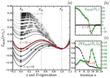
Figure 1: (a) Convergence of the McWeeny Lagrangian and density matrix eigenvalues during the course of the minimization using a test Hamiltonian and an occupation factor $\theta=0.10$. A grey scale is used to guide the eye during the processus of purification. Each curve is a plot of the function $\mathcal{L}_{\text{McW}}(x;\gamma_{n})$ computed at each iteration $n$. The red line correspond to $\mathcal{L}_{\text{McW}}(x;0)=\Omega_{\text{McW}}$. (b) Convergence of $\mathcal{L}_{\text{McW}}$ (green circles), and the trace conservation $\textrm{Tr}\{D_{n}\}-N$ (black dots). (c) Convergence of $\|\nabla\mathcal{L}_{\text{McW}}\|_{\mathcal{F}}$ (green circles) and $\|D_{n}\|_{\mathcal{F}}-N$ (black dots).

The parameter $c$ [Eq. (7b)] is recognized as the unstable fixed point introduced in Ref. [Palser and Manolopoulos, 1998], where $c\in[0,1]$. As a result, the interval $[-\frac{1}{3},\frac{1}{3}]$ constitutes the stable variational domain of $\gamma$.

The variation of the McWeeny Lagrangian function and the density matrix eigenvalues during the course of the minimization are presented in Fig. 1a for a test Hamiltonian with $N=10$, $M=100$, and a suitably conditioned initial guess (vide infra). The corresponding convergence profiles of $\mathcal{L}_{\text{McW}}$ and $\|\nabla\mathcal{L}_{\text{McW}}\|$ (green circles) are reported on Figs 1b and 1c, respectively, along with the trace conservation $\textrm{Tr}\{D_{n}\}-N$, and the density matrix norm convergence $\|D_{n}\|-N$ (black dots). We may notice first that for $\gamma=0$ (or $c=x_{m}=\frac{1}{2}$), $\mathcal{L}_{\text{McW}}$ simplifies to $\Omega_{\text{McW}}$. For intermediate states, $\gamma\in]-\frac{1}{3},0[\cup]0,\frac{1}{3}[$, the symmetry of $\Omega_{\text{McW}}$ is lost and the shape of $\mathcal{L}_{\text{McW}}(x,\gamma_{n})$ drives the eigenvalues in the left or in the right well. We may call them the hole and particle well, respectively. From the grey scale in Fig. 1a, we observe how $\gamma_{n}$ influences $\mathcal{L}_{\text{McW}}$ (along the $y$-axis) at $x_{\bar{p}}$, and the abscissa of the second stationnary point $x_{m}$ which is free to move in $[x_{\bar{p}},x_{p}]$. This yields to transform the hole well from a local $(n=0)$ to a global $(n=15)$ minima (or conversely the particule well from a global to a local minima). At the boundary values $\gamma=\{-\frac{1}{3},\frac{1}{3}\}$, $x_{\bar{p}}$ and $x_{m}$ merged to a saddle point in such a way that only one global minima left at $x_{p}$. Notice that, for situations where $\gamma\notin[-\frac{1}{3},\frac{1}{3}]$, the saddle point transforms to a maximum and runaway solutions may appear. Nevertheless, as long as $D_{0}$ is well conditioned, such kind of critical problem should not be encountered.

Figs. 1b and 1c highlight the minimization mechanism: (i) From iterate $n=0$ to $12$; $\gamma\rightarrow 0^{+}:$ $\mathcal{L}_{\text{McW}}$ follows the search direction and decreases monotonically. (ii) At iterate $n=13$; $\gamma\simeq 0:$ $\mathcal{L}_{\text{McW}}$ is close to the target value but the gradient residual is nonzero. (iii) From $n=14$ to 15; $\gamma<0:$ the search direction is inverted. (iv) At iterate $n=16$: all the eigenvalues are trapped in their respective wells. (iii) From iterate $n=17$ to $23$, $\gamma\rightarrow 0^{-}:$ we are in the McWeeny regime [Eq. (4)] and $\mathcal{L}_{\text{McW}}$ eventually reaches the global minimum.

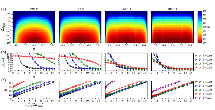
Figure 2: (a) Color maps displaying the average number of purifications ($\bar{p}$) as the function of the filling factor ($\theta$) and energy gap ($\Delta\epsilon_{\textrm{gap}}$). Results obtained from the PMCP and HPCP methods using the initial guess of Eqs. (2)-(11), and Eqs. (2)-(14) (notated PMCP+ and HPCP+). Each pixel on the maps correspond to an average over $32$ test Hamiltonians. (b) Energy convergence profiles with respect to the first 15 iterations for selected values of $\theta$. (c) Average number of purifications as a function of $\ln(1/\Delta\epsilon_{\textrm{gap}})$.

Taking advantage of the closure relation,

$$\bar{D}+D=I$$ (9)

where $\bar{D}$ stands for the hole density matrixMazziotti (2003), a more appealing form for the McWeeny canonical purification [Eq. (8)] can be derived by reformulating Eqs. (6a) and (7b) in terms of $D$ and $\bar{D}$:

$$D_{n+1}=D_{n}+2\left(D^{2}_{n}\bar{D}_{n}-\frac{\textrm{Tr}\{D^{2}_{n}\bar{D}_{n}\}}{\textrm{Tr}\{D_{n}\bar{D}_{n}\}}D_{n}\bar{D}_{n}\right)$$ (10)

Notice that since at convergence $D\bar{D}=0$, $\textrm{Tr}\{D\bar{D}\}$ must be chosen as the termination criterion in the recusion of Eq. (10) to avoid numerical instabilities when approaching the minima. The closed-form of this recurrence relation is remarkable: providing $\mathcal{H}$ used to build $D_{0}$ [Eq. (2)] and $N$, we have a self-consistent purification transformation which should converge to $\mathcal{D}$ without any support of heuristic adjustements. Indeed, Eq. (10) can also be derived from the PMCP relations by working on both $D$ and $\bar{D}$, and enforcing relation (9) at each iteration (see Appendix). Consequently, we can also demonstrateDianzinga et al. that the hole-particle canonical purification (HPCP) of Eq. (10) converges quadratically on $\mathcal{D}$ as shown on Fig. 2c.

To assess the efficiency and limitations of the HPCP, we have investigated the dependence of the number of purifications ($p$) on the occupation factor ($\theta$), and the energy gap $(\Delta\epsilon_{\textrm{gap}}=\epsilon_{N+1}-\epsilon_{N})$, defined by the higher-occupied ($\epsilon_{N}$) and lower-unoccupied ($\epsilon_{N+1}$) states. Similarly to the protocol of NiklassonNiklasson (2002, 2003), sequences of $M\times M$ dense Hamiltonian matrices ($M=100$) with vanishing off-diagonal elements were generated, having eigenvalues randomly distributed in the range $[-2.5,\epsilon_{N}]\cup[\epsilon_{N+1},2.5]$ for various $\Delta\epsilon_{\textrm{gap}}\in[10^{-7},1.0]$. As a first test, results are compared to the PMCPPalser and Manolopoulos (1998), along with the original initial guess [Eq. (2)], where:

$$\beta_{1}=\theta \quad\beta_{2}=\min\left\{\beta,\bar{\beta}\right\}$$ , (11)

with:

$$\beta=\frac{\theta}{\widetilde{\mathcal{H}}_{\textrm{max}}-\mu}, \quad\bar{\beta}=\frac{\bar{\theta}}{\mu-\widetilde{\mathcal{H}}_{\textrm{min}}},\quad\mu\simeq\widetilde{\mu}=\frac{\textrm{Tr}\{\mathcal{H}\}}{M}$$

and $\bar{\theta}=1-\theta=\bar{N}/M$, $\bar{N}$ being the number of unoccupied states. The lower and upper bounds of the Hamiltonian eigenspectrum ($\widetilde{\mathcal{H}}_{\textrm{min}}$ and $\widetilde{\mathcal{H}}_{\textrm{max}}$, respectively) were estimated from to the Geršgorin’s disc theoremGeršgorin (1931). The preconditioning of $D_{0}$ given in Eq. (11) guarantees that $\lambda(D_{0})\in[0,1]$, and gives rise to the following additional constraints:

$$\textrm{Tr}\{D_{0}\} =N$$ (12a)

$$\textrm{Tr}\{D_{0}\} >\textrm{Tr}\{D^{2}_{0}\}>\textrm{Tr}\{D^{3}_{0}\}$$ (12b)

$$\textrm{Tr}\{D^{3}_{0}\} >2\textrm{Tr}\{D^{2}_{0}\}-\textrm{Tr}\{D_{0}\}$$ (12c)

which are also necessary and sufficient conditions for $c\in[0,1]$ at the first iteration. Convergence was achieved with respect to the idempotency property, such that $\textrm{Tr}\{D_{n}\bar{D}_{n}\}\leq 10^{-6}$ for all the calculations. Additional tests on the Frobenius norm and the eigenvalues of the converged density matrix ($D_{\infty}$) were performed, using:

$$\|D_{\infty}\|_{\mathcal{F}}&-\sqrt{\textrm{Tr}\{D_{\infty}\}}<10^{-6}\\ \|D_{\infty}\|_{\mathcal{F}}-N<10^{-6}\\ \|\textrm{diag}\{D_{\infty}\}-\textrm{diag}\{I_{N},0_{\bar{N}}\}\|_{\mathcal{F}}<10^{-6}$$ (13)

which ensures that, at convergence, the representation of $D_{\infty}$ is orthogonal, and $D_{\infty}$ corresponds to the exact $N$-representable ground-state density matrix $\mathcal{D}$.

The variation of the average number of purifications ($\bar{p}$) with respect to $\theta$ and $\Delta\epsilon_{\textrm{gap}}$ are displayed on Fig. 2a using a color map for $\bar{p}\in[10,50]$. For a given energy gap, the HPCP shows a net improvement over the PMCP approach regarding moderate low and high occupation factors. Nevetheless, as previously noted by Niklasson and MazziottiNiklasson (2002); Mazziotti (2003), the extreme values of $\theta$ remain pathological for the original canonical purification, and to a lesser extent for the HPCP. One solution would be to break the symmetry of the McWeeny function by moving $x_{m}$ towards $x_{p}$ or $x_{\bar{p}}$ depending on the $\theta$ value. Basically, this requires a higher polynomial degree for $\Omega_{\text{McW}}$, ie. $\textrm{Tr}\{(D^{n}-D)^{2}\}_{n>2}$, resulting in a higher computational complexity. Assuming optimal programming, we emphasize that the PMCP and HPCP involved only two matrix multiplications per iteration. As already proved in Ref. [Palser and Manolopoulos, 1998], and highlighted by the energy convergence profiles in Fig. 2b, the PMCP and HPCP approach the (one particle) ground-state energy $\mathcal{E}=\textrm{Tr}\{\mathcal{H}\mathcal{D}\}$ monotonically, in other words, they are variational with respect to the Lagrange multiplier $\gamma$. The dependence of $\bar{p}$ on the band gap plotted in Fig. 2c confirms the early numerical experimentsNiklasson (2002); Rudberg and Rubensson (2011), where $\bar{p}$ increases linearly with respect to $\ln(1/\Delta\epsilon_{\textrm{gap}})$. The influence of $\theta$ is clearly apparent if we compare the minimum number of purification as required for the wider band gap ($y$-axis intercept), where for example, with $\theta=0.5$, both canonical purifications reach the ideal value of about 10 purifications, whereas for $\theta=0.05$, $\bar{p}_{\textrm{HPCP}}=23$ and $\bar{p}_{\textrm{PMCP}}=37$.

Let us consider how to improve the performance of the canonical purifications by working on the initial guess, regarding the hole-particle equivalence (or duality(Mazziotti, 2003)). Instead of searching for $D$, we may choose to purify $\bar{D}$, which simply requires replacing $D$ with $\bar{D}$ in the relation (10). In that case, the initial hole density matrix, satisfying $\lambda(\bar{D}_{0})\in[0,1]$, would be given by Eqs. (2) and (11), with $\beta_{1}=\bar{\theta}$ and $\beta_{2}=-\max\left\{\beta,\bar{\beta}\right\}$. Then, intuitively, the guess for the particle density matrix should be improved by using this additional information. Therefore, a more general preconditioning is proposed:

$$D^{+}_{0}=\alpha D_{0}+(1-\alpha)(I-\bar{D}_{0})$$ (14)

where $\alpha$ can be view as a mixing coefficient. Results obtained with this new precontionning are plotted in Fig. 2 (notated PMCP+ and HPCP+). As evident from Fig. 2a, the naive value of $\alpha=0.5$ leads to a net improvement of the PMCP and HPCP performances over the range $0.3<\theta<0.7$, inside of which the number of purifications becomes independent of $\theta$. Outside this interval, runaway solutions were encountered due to the ill-conditioning of $c$, where either of the constraints in Eq. (12b) or (12c) is violated. The solution to this problem is to perform a constrained search of $\alpha$ in Eq. (14), such that the first inequality of Eq. (12b) is respected, that is:

$$\underset{\begin{subarray}{c}0\leq\alpha\leq 1\\ \delta>0\end{subarray}}{\operatorname{search}}\>\left\{\textrm{Tr}\{D^{2}_{0}\}=\begin{cases}N-\delta N,\;\text{if}\>\theta<(1-\delta)\\ N-\delta\bar{N},\;\text{if}\>\theta>(1-\delta)\end{cases}\right\}$$ (15)

which leads to solve a second-order polynomial equation in $\alpha$, at the extra cost of only one matrix multiplication. Obviously, the parameter $\delta$ has to be carefully chosen such that the second equality of Eq. (12b) and condition (12c) are also respected. We found $\delta\simeq 2/3$ as the optimal valueDianzinga et al. . From Fig. 2, the benefits of this optimized preconditioning are clear when focussing within the range $]0.0,0.3]\cup[0.7,1.0[$, albeit with one or two extra purifications around the poles $\theta=\{0.3,0.7\}$ required to achieve the desired convergence. These benefits are even clearer in Fig. 2c, where we also show the plots of $\bar{p}$ as a function of $\ln(1/\Delta\epsilon_{\textrm{gap}})$ for the test case $\theta=0.01$. At the intercept we find $\bar{p}_{\textrm{PMCP}}\simeq 38$ compared to $\bar{p}_{\textrm{HPCP}}\simeq 21$, showing the improvment bring by the hole-particle equivalence. We have also compared our method against the most efficient of the trace updating methods, TRS4Niklasson et al. (2003), and find that for non-pathological fillings, the two are comparable in efficiency. For the pathological cases, where TRS4 adjusts the polynomial, it is more efficient, but at the expense of non-variational behaviour in the early iterations.

To conclude, we have shown how, by considering both electron and hole occupancies, the density matrix for a given system can be found efficiently while preserving $N$-representability. This opens the door to more robust, stable ground state minimisation algorithm, with application to standard and linear scaling DFT approaches.

Appendix A Alternative derivation of the hole-particle canonical purification

We demonstrate that by symmetrizing the Palser and Manolopoulos (PM) relations [Eqs. (16) of Ref. [Palser and Manolopoulos, 1998]] with respect to the hole density matrix, the closed-form of Eq. (10) appears naturally. Throughout the demonstration, quantities related to unoccupied subspace are indicated by a bar accent. Let us start from PM equations:

for $$c_{n}\leq\frac{1}{2}:$$ (16a)

$$D_{n+1}=-\frac{1}{1-c_{n}}D_{n}^{3}+\frac{1+c_{n}}{1-c_{n}}D_{n}^{2}+\frac{1-2c_{n}}{1-c_{n}}D_{n}$$

for $$c_{n}>\frac{1}{2}:$$ (16b)

$$D_{n+1}=-\frac{1}{c_{n}}D_{n}^{3}+\frac{1+c_{n}}{c_{n}}D_{n}^{2}$$

with $c_{n}$ given in Eq. (7b). We may search for purification relations dual to Eq. (16), ie. function of $\bar{D}$. We obtain:

for $$\bar{c}_{n}\geq\frac{1}{2}:$$ (17a)

$$\bar{D}_{n+1}=-\frac{1}{1-\bar{c}_{n}}\bar{D}_{n}^{3}+\frac{1+\bar{c}_{n}}{1-\bar{c}_{n}}\bar{D}_{n}^{2}+\frac{1-2\bar{c}_{n}}{1-\bar{c}_{n}}\bar{D}_{n}$$

for $$\bar{c}_{n}<\frac{1}{2}:$$ (17b)

$$\bar{D}_{n+1}=-\frac{1}{\bar{c}_{n}}\bar{D}_{n}^{3}+\frac{1+\bar{c}_{n}}{\bar{c}_{n}}\bar{D}_{n}^{2}$$

with $\bar{c}_{n}=1-c_{n}$. Instead of purifying either $D$ or $\bar{D}$, we shall try to take advantage of the closure relation [Eq. (9)] in such a way that, if we choose to work within the subspace of occupied states, the purification of $D$ [Eq. (16)] is constrained to verify $D=I-\bar{D}$. By inserting this constraint in Eq. (17), we obtain:

$$\textrm{for}\ \ c_{n}\leq\frac{1}{2}:&\ \ D_{n+1}=I-\left(-\frac{1}{c_{n}}(I-D_{n})^{3}\ +\frac{2-c_{n}}{c_{n}}(I-D_{n})^{2}-\frac{1-2c_{n}}{c_{n}}(I-D_{n})\right)\\ \textrm{for}\ \ c_{n}>\frac{1}{2}:\ \ D_{n+1}=I-\left(-\frac{1}{1-c_{n}}(I-D_{n})^{3}+\frac{2-c_{n}}{1-c_{n}}(I-D_{n})^{2}\right)$$ (18)

On multiplying Eqs. (16a) and (18) by $(1-c_{n})$ and $c_{n}$, respectively [or multiplying Eq. (16b) and (18) by $c_{n}$ and $(1-c_{n})$], and adding, we obtain:

$$D_{n+1}&=D_{n}+2\left(D^{2}_{n}\bar{D}_{n}-c_{n}D_{n}\bar{D}_{n}\right)$$ (19)

References

- McWeeny (1956a) R. McWeeny, Proc. R. Soc. Lond. A 235, 496 (1956a).
- McWeeny (1956b) R. McWeeny, Proc. R. Soc. Lond. A 237, 355 (1956b).
- McWeeny (1957) R. McWeeny, Proc. R. Soc. Lond. A 241, 239 (1957).
- McWeeny (1960) R. McWeeny, Rev. Mod. Phys. 32, 335 (1960).
- Li et al. (1993) X.-P. Li, R. W. Nunes, and D. Vanderbilt, Phys. Rev. B 47, 10891 (1993).
- Daniels et al. (1997) A. D. Daniels, J. M. Millam, and G. E. Scuseria, J. Chem. Phys. 107, 425 (1997).
- Millam and Scuseria (1997) J. M. Millam and G. E. Scuseria, J. Chem. Phys. 106, 5569 (1997).
- Daniels and Scuseria (1999) A. D. Daniels and G. E. Scuseria, J. Chem. Phys. 110, 1321 (1999).
- Bowler and Gillan (1999) D. Bowler and M. Gillan, Comp. Phys. Comm. 120, 95 (1999).
- Challacombe (1999) M. Challacombe, J. Chem. Phys. 110, 2332 (1999).
- Goedecker and Colombo (1994) S. Goedecker and L. Colombo, Phys. Rev. Lett. 73, 122 (1994).
- Goedecker and Teter (1995) S. Goedecker and M. Teter, Phys. Rev. B 51, 9455 (1995).
- Baer and Head-Gordon (1997a) R. Baer and M. Head-Gordon, Phys. Rev. Lett. 79, 3962 (1997a).
- Baer and Head-Gordon (1997b) R. Baer and M. Head-Gordon, J. Chem. Phys. 107, 10003 (1997b).
- Bates et al. (1998) K. R. Bates, A. D. Daniels, and G. E. Scuseria, J. Chem. Phys. 109, 3308 (1998).
- Liang et al. (2003) W. Liang, C. Saravanan, Y. Shao, R. Baer, A. T. Bell, and M. Head-Gordon, J. Chem. Phys. 119, 4117 (2003).
- Niklasson (2003) A. M. N. Niklasson, Phys. Rev. B 68, 233104 (2003).
- Németh and Scuseria (2000) K. Németh and G. E. Scuseria, J. Chem. Phys. 113, 6035 (2000).
- Beylkin et al. (1999) G. Beylkin, N. Coult, and M. J. Mohlenkamp, J. Comput. Phys. 152, 32 (1999).
- Kenney and Laub (1991) C. Kenney and A. Laub, SIAM. J. Matrix Anal. & Appl. 12, 273 (1991).
- Niklasson (2002) A. M. N. Niklasson, Phys. Rev. B 66, 155115 (2002).
- Niklasson et al. (2003) A. M. N. Niklasson, C. J. Tymczak, and M. Challacombe, J. Chem. Phys. 118, 8611 (2003).
- Palser and Manolopoulos (1998) A. H. R. Palser and D. E. Manolopoulos, Phys. Rev. B 58, 12704 (1998).
- Bowler and Miyazaki (2012) D. R. Bowler and T. Miyazaki, Rep. Prog. Phys. 75, 036503 (2012).
- Goedecker (1999) S. Goedecker, Rev. Mod. Phys. 71, 1085 (1999).
- Parr and Weitao (1994) R. G. Parr and Y. Weitao, Density-Functional Theory of Atoms and Molecules (Oxford University Press, New York; Oxford England, 1994).
- Rudberg and Rubensson (2011) E. Rudberg and E. H. Rubensson, J. Phys.: Condens. Matter 23, 075502 (2011).
- Chow et al. (2015) E. Chow, X. Liu, M. Smelyanskiy, and J. R. Hammond, J. Chem. Phys. 142, 104103 (2015).
- Cawkwell et al. (2012) M. J. Cawkwell, E. J. Sanville, S. M. Mniszewski, and A. M. N. Niklasson, J. Chem. Theory Comput. 8, 4094 (2012).
- Cawkwell et al. (2014) M. J. Cawkwell, M. A. Wood, A. M. N. Niklasson, and S. M. Mniszewski, J. Chem. Theory Comput. 10, 5391 (2014).
- Note (1) We will restrict our discussion to effective one-electron Hamiltonian operators expressed in a finite orthonormal Hilbert space. It does not pose severe challenge to generalize the demonstration to a non-orthogonal basis set.
- Mazziotti (2003) D. A. Mazziotti, Phys. Rev. E 68, 066701 (2003).
- (33) R. M. Dianzinga, L. A. Truflandier, and D. R. Bowler, unpublished results .
- Geršgorin (1931) S. Geršgorin, Proc. USSR Acad. Sci. 51, 749 (1931).
- Note (2) The Frobenius norm is defined by: Notice that: , such that , then .
- Note (3) In that case it can be shown that: .