Detection of zeptojoule microwave pulses using electrothermal feedback in proximity-induced Josephson junctions

Abstract

We experimentally investigate and utilize electrothermal feedback in a microwave nanobolometer based on a normal-metal ($\textnormal{Au}_{x}\textnormal{Pd}_{1-x}$) nanowire with proximity-induced superconductivity. The feedback couples the temperature and the electrical degrees of freedom in the nanowire, which both absorbs the incoming microwave radiation, and transduces the temperature change into a radio-frequency electrical signal. We tune the feedback in situ and access both positive and negative feedback regimes with rich nonlinear dynamics. In particular, strong positive feedback leads to the emergence of two metastable electron temperature states in the millikelvin range. We use these states for efficient threshold detection of coherent $8.4\mbox{ GHz}$ microwave pulses containing approximately 200 photons on average, corresponding to $1.1\times 10^{-21}\textnormal{ J}\approx 7.0\textnormal{ meV}$ of energy.

Superconducting qubits coupled to microwave transmission lines have developed into a versatile platform for solid-state quantum optics experiments Blais et al. (2004); Wallraff et al. (2004), as well as a promising candidate for quantum computing Devoret and Schoelkopf (2013); Kelly et al. (2015). However, compared to optical photodetectors Lita et al. (2008); Marsili et al. (2013); Eisaman et al. (2011), detectors for itinerant single-photon microwave pulses are still in their infancy. This prevents microwave implementations of optical protocols that require feedback conditioned on single-photon detection events. For example, linear optical quantum computing with single-photon pulses calls for such feedback Kok et al. (2007). Photodetection and feedback can also act as a quantum eraser Hillery and Scully (1983) of the phase information available in a coherent signal, as we recently discussed in Ref. Govenius et al. (2015). Note that, given sufficient averaging, linear amplifiers can substitute for photodetectors in ensemble-averaged experiments da Silva et al. (2010); Bozyigit et al. (2010), but the uncertainty principle fundamentally limits the success probability in single-shot experiments.

We focus on thermal photodetectors, i.e., detectors that measure the temperature rise caused by absorbed photons. Thermal detectors have been developed for increasingly long wavelengths in the context of THz astronomy Karasik et al. (2011), the record being the detection of single $8\textnormal{ $\mu$m}$ photons Karasik et al. (2012). In the context of quantum thermodynamics Pekola (2015), thermal detectors have recently been proposed Pekola et al. (2013) and developed Schmidt et al. (2003, 2005); Gasparinetti et al. (2015); Saira et al. as monitorable heat baths.

The other main approach to detecting itinerant microwave photons is to use a qubit that is excited by an incoming photon and then measured Romero et al. (2009); Chen et al. (2011); Peropadre et al. (2011); Fan et al. (2013); Hoi et al. (2013); Sathyamoorthy et al. (2014); Fan et al. (2014); Koshino et al. (2015); Inomata et al. ; Narla et al. . Very recently, Ref. Inomata et al. reported reaching an efficiency of 0.66 and a bandwidth of roughly 20 MHz using such an approach. Use of qubit-based single-photon transistors as photodetectors has also been proposed Neumeier et al. (2013); Manzoni et al. (2014). If the pulse is carefully shaped, it is also possible to efficiently absorb a photon into a resonator Cirac et al. (1997); Yin et al. (2013); Srinivasan et al. (2014); Wenner et al. (2014); Pechal et al. (2014). There it could be detected with established techniques for intra-resonator photon counting Gleyzes et al. (2007); Sun et al. (2014).

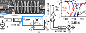
Figure 1: (Color online) (a) Simplified diagram of the detector, including (b) a micrograph of the SNS junctions formed by a $\textnormal{Au}_{x}\textnormal{Pd}_{1-x}$ nanowire contacted by Al islands and leads ($H$, $P$, and $G$). Here, $Z^{-1}$ is an admittance, $T_{e}$ is the temperature of the electrons in the nanowire, and $\Gamma$ is the probe signal reflection coefficient. The micrograph is from a device nominally identical to the measured one. (c) Reflected fraction of probe power versus probe frequency $f_{\textnormal{p}}$ for steady-state heating power $P_{\textnormal{h}}$ of $1.9$, $66$, and $290\mbox{ aW}$. They are measured at low probe power $P_{\textnormal{p}}\ll P_{\textnormal{h}}$. The solid curves are fits to the circuit model with a small phenomenological correction term Note (1). The heater input is bandpass filtered ($8.41\pm 0.02\textnormal{ GHz})$.

The main advantage of thermal detectors is that they typically present a suitable real input impedance for absorbing photons efficiently over a wide bandwidth and a large dynamic range, in contrast to qubit-based detectors. However, a central problem in the thermal approach is the small temperature rise caused by individual microwave photons. The resulting transient temperature spike is easily overwhelmed by noise added in the readout stage. One potential solution is to use a bistable system as a threshold detector that maps a weak transient input pulse to a long-lived metastable state of the detector. This is conceptually similar to, e.g., early experiments on superconducting qubits that used a current-biased superconducting quantum interference device (SQUID) Chiorescu et al. (2003). Conditioned on the initial qubit state, the SQUID either remained in the superconducting state or switched to a long-lived non-zero voltage state.

In this Letter, we show that an electrothermal bistability emerges in the microwave nanobolometer we introduced in Ref. Govenius et al. (2014) and that it enables high-fidelity threshold detection of $8.4\mbox{ GHz}$ microwave pulses containing only $200\times h\times 8.4\,\textnormal{GHz}\approx 1.1\textnormal{ zJ}$ of energy. This threshold is more than an order of magnitude improvement over previous thermal detector results Santavicca et al. (2010); Karasik et al. (2012). The bistability in our detector arises from the fact that the amount of power absorbed from the electrical probe signal used for readout depends on the measured electron temperature itself. Previously, such electrothermal feedback and the associated bifurcation has been studied in the context of kinetic inductance detectors de Visser et al. (2010); Thompson et al. (2013); Lindeman (2014); Thomas et al. (2015). Analogous thermal effects in optics are also known Braginsky et al. (1989); Fomin et al. (2005). The main difference to our device is the relative strength of the electrothermal effect, which in our case leads to strongly nonlinear behavior at attowatt probe powers. Electrothermal feedback is also commonly used in transition edge sensors Karasik et al. (2011), but typically the feedback is chosen to be negative because that suppresses Johnson noise and leads to fast self-resetting behavior Irwin (1995).

The central component of our detector (Fig. 1) is a metallic $\textnormal{Au}_{x}\textnormal{Pd}_{1-x}$ nanowire ($x\approx 0.6$) contacted by three Al leads ($H$, $P$, and $G$) and seven Al islands that are superconducting at millikelvin temperatures . The longest superconductor–normal-metal–superconductor (SNS) junction ($H$–$G$) provides a resistive load ($36\textnormal{ $\Omega$}$) for the radiation to be detected Nahum and Martinis (1993), while the shorter junctions ($P$–$G$) function as a proximity Josephson sensor Giazotto et al. (2008); Voutilainen et al. (2010). That is, the shorter junctions provide a temperature-dependent inductance in an effective LC resonator used for readout. Because the inductance increases with electron temperature $T_{e}$ in the nanowire, the resonance frequency shifts down as the heating power $P_{\textnormal{h}}$ increases. Therefore the detector transduces changes in $P_{\textnormal{h}}$ into changes in the reflection coefficient $\Gamma$ [Fig. 1(c)]. For simplicity, we limit the bandwidth of the heater line using a Lorentzian bandpass filter, but replacing it with a wider band filter should be straightforward.

We first characterize the detector by measuring the $P_{\textnormal{h}}$-dependence of the admittance $Z^{-1}$ between $P$ and $G$. To do so, we fit the measured $\Gamma$ to a circuit model in which we parametrize $Z^{-1}$ as $R^{-1}+(i\omega L)^{-1}$, where $\omega/2\pi=f_{\textnormal{p}}$ is the probe frequency. The circuit model shown in Fig. 1(a) predicts $\Gamma=(Z_{\textnormal{L}}-Z_{0})/(Z_{\textnormal{L}}+Z_{0})$, where

$$Z_{\textnormal{L}}=(i\omega C_{\textnormal{g}})^{-1}+\{i\omega C_{2}+[(i\omega C_{1})^{-1}+Z(T_{e})]^{-1}\}^{-1},$$

$Z_{0}=50\textnormal{ $\Omega$}$, $C_{1}\approx 87\textnormal{ pF}$, $C_{2}\approx 70\textnormal{ pF}$, and $C_{\textnormal{g}}\approx 1.5\textnormal{ pF}$. This fits reasonably well to the linear response data shown in Fig. 1(c). However, in order to reproduce the asymmetry in the measured lineshape, we add a small frequency-dependent correction to the model Note (1). Here, linear response refers to the use of a probe power $P_{\textnormal{p}}$ low enough to ignore both the electrical and electrothermal nonlinearities, i.e., the nonlinearity of the Josephson inductance as well as the variation of $T_{e}$ as a function of the absorbed probe power $(1-\left|\Gamma\right|^{2})P_{\textnormal{p}}$. We note that the uncertainty in $P_{\textnormal{h}}$ is roughly $1\textnormal{ dB}$ Note (1), and that dissipation in the capacitors is negligible.

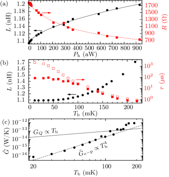
Figure 2: (Color online) Linear ($P_{\textnormal{p}}\ll P_{\textnormal{h}}$ ) response. (a) The effective inductance (circles) and resistance (squares) of the short SNS junctions as functions of external steady-state heating power $P_{\textnormal{h}}$. The bath temperature $T_{\textnormal{b}}$ is $12\textnormal{ mK}$. The curves are phenomenological fits that allow mapping a measured reflection coefficient into an equivalent $P_{\textnormal{h}}$. (b) The effective inductance (circles) and thermal relaxation time after a short (filled squares) or long (open squares) heating pulse. (c) Measured differential thermal conductance $\tilde{G}$, the expected electron-phonon contribution $\tilde{G}_{e-\textnormal{p}}$ (dashed line), and the quantum of thermal conductance $G_{Q}$ (solid line).

Figure 2(a) shows the extracted linear response $L$ and $R$ for heating powers up to a femtowatt. Figure 2 also shows the bath temperature dependence of $L$, the thermal relaxation time $\tau$, and the differential thermal conductance $\tilde{G}=-\partial_{T_{\textnormal{b}}}P_{e-\textnormal{b}}\left(T_{e},T_{\textnormal{b}}\right)$ Note (1). Here, $P_{e-\textnormal{b}}\left(T_{e},T_{\textnormal{b}}\right)$ is the heat flow between the electrons in the nanowire and the cryostat phonon bath at temperature $T_{\textnormal{b}}$. The measured $\tilde{G}$ is in rough agreement with the prediction for electron–phonon limited thermalization $\tilde{G}_{e-\textnormal{p}}=5\Sigma V_{0}T_{\textnormal{b}}^{4}$, where $\Sigma\approx 3\times 10^{9}\textnormal{ W/m}^{3}\textnormal{K}^{5}$ is a material parameter Timofeev et al. (2009) and $V_{0}\approx\left(240\textnormal{ nm}\right)^{3}$ is the volume of the part of the nanowire not covered by Al. We can use these results to estimate $C_{e}$ above $100\textnormal{ mK}$, where $T_{e}\approx T_{\textnormal{b}}$ and $C_{e}\approx\tau\tilde{G}\approx\gamma V_{0}T_{\textnormal{b}}$, with $\gamma V_{0}=8\textnormal{ aJ/K}^{2}$ Note (1).

Below $100\textnormal{ mK}$, the relaxation toward the stationary state is faster after a short ($1\textnormal{ $\mu$s}$) heating pulse than after a long ($\gg\tau$) heating pulse Note (1). Therefore, the simplest thermal model of a single heat capacity $C_{e}$ coupled directly to the bath is not accurate below $100\textnormal{ mK}$. Instead, the second time scale can be phenomenologically explained by an additional heat capacity $C^{\prime}\gg C_{e}$ coupled strongly to $C_{e}$ but weakly to the bath, as compared to $\tilde{G}$. Since $\tilde{G}$ falls far below the quantum of thermal conductance $G_{Q}=\pi^{2}k_{\textnormal{B}}^{2}T_{\textnormal{b}}/3h$ Pendry (1983) at low temperatures [Fig. 2(c)], even weak residual electromagnetic coupling Schmidt et al. (2004); Meschke et al. (2006); Partanen et al. (2016) between $C_{e}$ and $C^{\prime}$ would suffice. However, we cannot uniquely determine the microscopic origin of $C^{\prime}$ or the coupling mechanism from the data. Also note that a similar second time scale was observed in Ref. Gasparinetti et al. (2015).

At high probe powers, the linear-response behavior studied above may be drastically modified by the absorbed probe power. Below we focus on the stationary $T_{e}$ solutions, so we choose to neglect the transient heat flows to $C^{\prime}$ that give rise to the shorter time scale in Fig. 2(b). Similarly, we neglect the contribution of electrical transients to $\Gamma$, as they decay even faster (in $\apprle 100\,\mbox{ns}$). Under these approximations, $T_{e}$ is the only dynamic variable and evolves according to

$$C_{e}\left(T_{e}\right)\dot{T}_{e} =-P_{e-\textnormal{b}}\left(T_{e},T_{\textnormal{b}}\right)+P_{x}+P_{\textnormal{h}}$$ (1)

$$\qquad+(1-\left|\Gamma\left(T_{e},\omega\right)\right|^{2})P_{\textnormal{p}},$$

where $P_{x}$ accounts for the average heat load from uncontrolled sources.

Determining $T_{e}$ from Eq. (1) and the measured $\Gamma$ would require additional assumptions about $P_{e-\textnormal{b}}$ and $P_{x}$, as they are not directly measurable. However, we avoid making such assumptions by instead analyzing the increase in the heat flow from the electrons to the thermal bath, as compared to the case $P_{\textnormal{h}}=P_{\textnormal{p}}=0$. That is, instead of $T_{e}$, we analyze

$$\Delta(T_{e})=P_{e-\textnormal{b}}(T_{e},T_{\textnormal{b}})-P_{x},$$ (2)

which is monotonic in $T_{e}$. Given this definition, we can rewrite Eq. (1) as

$$\tau\left(\Delta\right)\dot{\Delta}=-\Delta+P_{\textnormal{h}}+(1-\left|\Gamma\left(\Delta,\omega\right)\right|^{2})P_{\textnormal{p}},$$ (3)

where $\tau\left(\Delta\right)=C\left(\Delta\right)/\partial_{T_{e}}P_{e-\textnormal{b}}\textnormal{{(}}T_{e}(\Delta),T_{\textnormal{b}}\textnormal{{)}}$. In contrast to the unknown parameters in Eq. (1), $\Gamma\left(\Delta,\omega\right)$ and $\tau\left(\Delta\right)$ are directly measurable in linear response. Specifically, we can determine $\Gamma\left(\Delta,\omega\right)$ from the data in Fig. 2(a) since $\Delta=P_{\textnormal{h}}$ when $P_{\textnormal{p}},\dot{\Delta}\rightarrow 0$. By inverting $\Gamma\left(\Delta,\omega\right)$, we can then extract $\Delta$ from the measured $\Gamma$. Also note that, since all parameters in Eq. (3) are determined in linear response, no free parameters remain in the theoretical predictions for the nonlinear case discussed below.

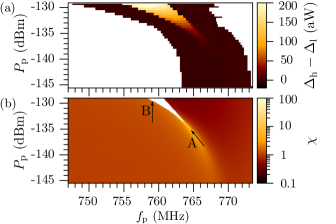
Figure 3: (Color online) (a) Bistable parameter regime, as indicated by a non-zero difference $\Delta_{\textnormal{h}}-\Delta_{\textnormal{l}}$ in the power absorbed from the probe signal in high and low-temperature stationary states. (b) Numerically simulated values of the dimensionless susceptibility to external heating $\chi$ in the single-valued regime. The bistable regime is indicated in white.

The emergence of bistability is the most dramatic consequence of increasing the probe power. Experimentally, we map out the bistable parameter regime by measuring the difference $\Delta_{\textnormal{h}}-\Delta_{\textnormal{l}}$ as a function of $f_{\textnormal{p}}$ and $P_{\textnormal{p}}$ [Fig. 3(a)]. Here, $\Delta_{\textnormal{h}}$ $\left(\Delta_{\textnormal{l}}\right)$ corresponds to the ensemble-averaged $\Delta$ measured $5\textnormal{ ms}$ after preparing the system in a high-$\Delta$ (low-$\Delta$) initial state. We then identify the region of non-zero $\Delta_{\textnormal{h}}-\Delta_{\textnormal{l}}$ as the regime where $\Delta$ (and hence $T_{e}$) is bistable. This method is approximate mainly because the lifetimes of the metastable states may be short compared to $5\textnormal{ ms}$.

Figure 3(b) shows the theoretical prediction for the bistable region in white. We generate it by numerically finding the stationary solutions of Eq. (3), with $\Gamma\left(\Delta,\omega\right)$ determined from the fits shown in Fig. 2(a) Note (1). The qualitative features of the prediction agree well with the experimental results. Quantitatively, the measured bistable regime broadens in frequency faster than the predicted one. This discrepancy is most likely due to imperfect impedance matching of the probe line and the imperfect correspondence between bistability and $\Delta_{\textnormal{h}}-\Delta_{\textnormal{l}}\neq 0$.

The non-white areas in Fig. 3(b) show the prediction for the susceptibility of the stationary-state $\Delta$ to external heating, i.e., $\chi=\left.\partial\Delta/\partial P_{\textnormal{h}}\right|_{\dot{\Delta}=0}.$ It is a convenient dimensionless way to quantify the importance of the electrothermal nonlinearity. Besides characterizing susceptibility to heating, $\chi$ also gives the ratio of the effective thermal time constant to its linear response value. Figure 3(b) shows that both positive ($\chi\gg 1$) and negative ($\chi\ll 1$) feedback regimes are accessible by simply choosing different values of $f_{\textnormal{p}}$ and $P_{\textnormal{p}}$.

There are two distinct ways to operate the device as a detector in the nonlinear regime. Approaching the bistable regime along line A in Fig. 3, the system undergoes a pitchfork bifurcation preceded by a diverging $\chi$. Analogously to the linear amplification of coherent pulses by a Josephson parametric amplifier Zimmer (1967); Castellanos-Beltran and Lehnert (2007), our device could in principle detect heat pulses in a continuous and energy-resolving manner in this regime preceding the bifurcation. However, the focus of this paper is threshold detection, which uses the imperfect pitchfork bifurcation encountered along line B in Fig. 3 and bears a closer resemblance to the Josephson bifurcation amplifier (JBA) Siddiqi et al. (2004); Vijay et al. (2009).

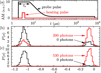
Figure 4: (Color online) (a) Amplitude modulation (AM) of the probe pulse used for detecting weak $1\,\mu\textnormal{s}$ heating pulses (also shown). The carrier frequencies are $757\textnormal{ MHz}$ and $8.4\textnormal{ GHz}$ for the probe and heating pulses, respectively. (b) Normalized histograms of the single-shot measurement outcome $s$ with a heating pulse energy of zero or $200\times h\times 8.4\,\textnormal{GHz}\approx 1.1\textnormal{ zJ}$. The pulses for the two histograms were interleaved in time. (c) Same as (b) but for $3.0\textnormal{ zJ}$ and $t_{\textnormal{s}}=2.5\textnormal{ $\mu$s}$.

In the threshold detection mode, we modulate the probe signal amplitude as shown in Fig. 4(a) while keeping the probe frequency fixed at $f_{\textnormal{p}}=757\textnormal{ MHz}$. The amplitude modulation pattern first initializes the system to a low-$\Delta$ state, then makes it sensitive to a transition to the high-$\Delta$ state for roughly $t_{\textnormal{s}}\approx 4.5\textnormal{ $\mu$s}$ during which the heating pulse is sent, and finally keeps the system in a long-lifetime part of the bistable regime for another $7\textnormal{ ms}$ in order to time-average the output signal. During the last stage $P_{\textnormal{p}}\approx-131\textnormal{ dBm}$. This is similar to how JBAs operate Vijay et al. (2009). Note, however, that the probe and heater signals do not interfere coherently due to the transduction through electron temperature. That is, at heater frequencies well above $\tau^{-1}$, the output signal is independent of the phase of the heater signal.

The histograms in Fig. 4(b,c) show that the detector switches reliably to the high-temperature state with a heating pulse energy $E_{\textnormal{pulse}}\apprge 1\textnormal{ zJ}$, while it typically remains in the low-temperature state if no heating is applied. The histograms are plotted against $s=\textnormal{Re}\left[e^{1.482\pi i}\int_{0.8\textnormal{ ms}}^{6.4\textnormal{ ms}}dt\Gamma\left(t\right)/\left(5.6\textnormal{ ms}\right)\right]$, i.e., a projection of the time-averaged reflection coefficient. Few switching events occur during the averaging time, as indicated by the scarcity of points between the two main peaks in the probability density $P\left(s\right)$. Instead, the errors arise from spurious early switching events and events where the detector does not switch despite a heating pulse. In particular, for a heat pulse of approximately 200 photons, the readout fidelity is $F=0.56$ [Fig. 4(b)]. Here, $F=1-P\left(s>-0.25|\textnormal{no heat pulse}\right)-P\left(s\leq-0.25|\textnormal{heat pulse}\right)$. For a heat pulse of 530 photons, $F=0.94$ [Fig. 4(c)]. For 330 photons, $F=0.75$ Note (1).

The observed pulse energy dependence of $F$ is in agreement with the errors arising mainly from Gaussian fluctuations in the energy of the nanowire electrons. Such fluctuations limit $F$ to $\bar{F}=\textnormal{erf}(2^{-3/2}E_{\textnormal{pulse}}/\Delta E_{\textnormal{RMS}})$, even for ideal instantaneous threshold detection. For RMS fluctuations $\Delta E_{\textnormal{RMS}}=0.7\textnormal{ zJ}$, $\bar{F}$ agrees well with the above mentioned values of $F$. This phenomenological $\Delta E_{\textnormal{RMS}}$ should be compared to the thermodynamic fluctuations $\Delta E_{\textnormal{RMS}}^{\prime}=\sqrt{k_{\textnormal{B}}T_{e}^{2}C_{e}}$ in the absence of electrothermal feedback Moseley et al. (1984). For $T_{e}=50\textnormal{ mK}$, we estimate $C_{e}\approx 400\textnormal{ zJ/K}$, leading to $\Delta E_{\textnormal{RMS}}^{\prime}\approx 0.12\textnormal{ zJ}\approx C_{e}\times 0.29\textnormal{ mK}$. This suggests that the thermodynamic fluctuations are a significant, even if not the dominant, fidelity-limiting factor. Note that, although the feedback during the pulse sequence in Fig. 4(a) is strong and positive, all signals are kept off for at least $400\textnormal{ ms}$ before each probe pulse. Therefore, the fluctuations just before the brief period relevant for switching ($t_{\textnormal{s}}\ll\tau$) are not affected by the electrothermal feedback.

In conclusion, we have experimentally investigated the electrothermal feedback effect in a microwave photodetector. The results are in agreement with a simple model which we used to highlight that both strong positive and strong negative feedback is available by adjusting the probe power and frequency. We demonstrated that bistability emerges in the limit of extreme positive feedback and that it can be used for efficient threshold detection of weak microwave pulses at the zeptojoule level. This is more than an order of magnitude improvement over previous thermal detector results, and therefore an important step toward thermal detection of individual itinerant microwave photons. To reach the single-photon level, we should further reduce the nanowire volume and possibly replace $\textnormal{Au}_{x}\textnormal{Pd}_{1-x}$ by a material with lower specific heat. This would reduce the time constant as well as the thermodynamic energy fluctuations, which contribute significantly to the achieved fidelities according to our estimate. Furthermore, there seems to be room for technical improvement in shielding and filtering, which would bring the observed $\Delta E_{\textnormal{RMS}}$ closer to the thermodynamic fluctuations and would, most likely, lead to a lower electron temperature. Finally, a state-of-the-art amplifier Vijay et al. (2011); André et al. (1999); Macklin et al. (2015) on the probe output should reduce the required averaging time by at least two orders of magnitude Note (1).