Stabilization of Uncertain Discrete-time Linear System via Limited Information

Abstract

This paper proposes a procedure to control an uncertain discrete-time networked control system through a limited stabilizing input information. The system is primarily affected by the time-varying, norm bounded, mismatched parametric uncertainty. The input information is limited due to unreliability of communicating networks. An event-triggered based robust control strategy is adopted to capture the network unreliability. In event-triggered control the control input is computed and updated at the system end only when a pre-specified event condition is violated. The robust control input is derived to stabilize the uncertain system by solving an optimal control problem based on a virtual nominal dynamics and a modified cost-functional. The designed robust control law with limited information ensures input-to-sate stability (ISS) of original system under presence of mismatched uncertainty. Deriving the event-triggering condition for discrete-time uncertain system and ensuring the stability of such system analytically are the key contributions of this paper. A numerical example is given to prove the efficacy of the proposed event-based control algorithm over the conventional periodic one.

I Introduction

Controlling uncertain cyber-physical systems (CPS) or networked control systems (NCS) subjected to limited information is a challenging task. Generally in CPS or NCS, multiple physical systems are interconnected and exchanged their local information through a digital network. Due to shared nature of communicating network the continuous or periodic transmission of information causes a large bandwidth requirement. Apart from bandwidth requirement, most of the cyber-physical systems are powered by DC battery, so efficient use of power is essential. It is observed that transmitting data over the communicating network has a proportional relation with the power consumption. This trade off motivates a large number of researchers to continue their research on NCS with minimal sensing and actuation [1]-[11], [15]-[19]. Recently an event-triggered based control technique is proposed by [4]-[6], to reduce the information requirement for realizing a stabilizing control law. In event-triggered control, sensing at system end and actuation at controller end happens only when a pre-specified event condition is violated. This event-condition mostly depends on system’s current states or outputs. The primary shortcoming of continuous-time event-triggered control is that it requires a continuous monitoring of event condition. In [15]-[16], Heemels et al. proposes an event-triggering technique where event-condition is monitored periodically. To avoid continuous or periodic monitoring, self-triggered control technique is reported in [8]-[9] where the next event occurring instant is computed analytically based on the state of previous instant. Maximizing inter-event time is the key aim of the event-triggered or self-triggered control in order to reduce the total transmission requirements. A Girad [6], proposes a new event-triggering mechanism named as dynamic event-triggering to achieve larger inter-event time with respect to previous approach [4]. The above discussion says the efficacy of aperiodic sensing and actuation over the continuous or periodic one in the context of NCS [3].

In NCS, uncertainty is mainly considered in communicating network in the form of time-delay, data-packet loss in between transreceiving process [24], [30], [31]. On the other hand the unmodeled dynamics, time-varying system parameters, external disturbances are the primary sources of system uncertainty. The main shortcoming of the classical event-triggered system lies in the fact that one must know the exact model of the plant apriori. A system with an uncertain model is a more realistic scenario and has far greater significance. However, there are open problems of designing a control law and triggering conditions to deal with system uncertainties. To deal with parametric uncertainty, F. Lin et.al. proposes a continuous-time robust control technique where control input is generated by solving an equivalent optimal control problem [25]-[27]. The optimal control problem is formulated based on the nominal or auxiliary dynamics by minimizing a quadratic cost-functional which depends on the upper bound of uncertainty. The similar concepts is extended for nonlinear continuous system in [28], [29], where a non-quadratic cost-functional is considered. However, this framework for discrete-time uncertain system is not reported. Recently E. Garcia et.al. have proposed an event-triggered based discrete-time robust control technique for NCS [10]-[11]. To realize the robust control law their prior assumptions are that the physical system is affected by matched uncertainty (which is briefly discussed in section II) and the uncertainty is only in system’s state matrix. But considering mismatched uncertainty in both state and input matrices is more realistic control problem. This is due to the fact that, the existence of stabilizing control law can be guaranteed for matched uncertainty but difficult for mismatched system. Stabilization of mismatched uncertain system with communication constraint is a challenging task. This motivates us to formulate the present problem.
In this paper a novel discrete-time robust control technique is proposed for NCS, where physical systems are inter-connected through an unreliable communication link. Due to unavailability of network the robust control law is designed using minimal state information. The designed control law acts on the physical system where the state model is affected by mismatched parametric uncertainty. For mathematical simplicity we are avoiding other uncertainties like external disturbances, noises. The communication unreliability is resolved by considering an event-triggered control technique, where control input is computed and updated only when an event-condition is satisfied. To derive the discrete-time robust control input a virtual nominal system and a modified cost-functional is defined. Solution of the optimal control problem helps to design the stabilizing control input for uncertain system. The input-to-state stability (ISS) technique is used to derive the event-triggering condition and as well as to ensure the stability of closed loop system.

Highlights of contributions

The contributions of this paper are summarized as follows:

(i)

Present paper proposes a robust control framework for discrete time linear system where state matrix consists of mismatched uncertainty. The periodic robust control law is derived by formulating an equivalent optimal control problem. Optimal control problem is solved for an virtual system with a quadratic cost-functional which depends on the upper bound on uncertainty.

(ii)

The virtual nominal dynamics have two control inputs $u$ and $v$. The concept of virtual input $v$ is used to derive the existence of stabilizing control input $u$ to tackle mismatched uncertainty. The proposed robust control law ensures asymptotic convergence of uncertain closed loop system.

(iii)

An event-triggered robust control technique is proposed for discrete-time uncertain system, where controller is not collocated with the system and connected thorough a communication network. The aim of this control law is to achieve robustness against parameter variation with event based communication and control. The event condition is derived from the ISS based stability criteria.

(iv)

It is shown that some of the existing results of matched system is a special case of the proposed results [10]-[11]. A comparative study is carried out between periodic control over the event-triggered control on the numerical example.

Notation & Definitions

The notation $\|x\|$ is used to denote the Euclidean norm of a vector $x\in{\mathbb{R}^{n}}$. Here $\mathbb{R}^{n}$ denotes the $n$ dimensional Euclidean real space and $\mathbb{R}^{n\times{m}}$ is a set of all $(n\times{m})$ real matrices. $\mathbb{R}^{+}_{0}$ and $\mathbb{I}$ denote the all possible set of positive real numbers and non-negative integers. $X\leq{0}$, $X^{T}$ and $X^{-1}$ represent the negative definiteness, transpose and inverse of matrix $X$, respectively. Symbol $I$ represents an identity matrix with appropriate dimensions and time $t_{\infty}$ implies $+\infty$. Symbols $\lambda_{min}(P)$ and $\lambda_{max}(P)$ denote the minimum and maximum eigenvalue of symmetric matrix $P\in\mathbb{R}^{n\times n}$ respectively. Through out this paper following definitions are used to derived the theoretical results [32].

Definition 1.

A system

$$x(k+1)=Ax(k)+Bu(k)$$ (1)

is globally ISS if it satisfies

$$\|x(k)\|\leq\beta(\|x(0)\|,k)+\gamma\bigg{(}sup_{\tau\in[0,\infty)}\big{\{}\|u_{\tau}\|\big{\}}\bigg{)}$$ (2)

with each input $u(k)$ and each initial condition $x(0)$. The functions $\beta$ and $\gamma$ are $KL$ and $K_{\infty}$ functions respectively.

Definition 2.

A discrete-time system $x(k+1)=f(x,u,d)$, whose origin is an equilibrium point if $f(0,x)=0$ $\forall\ k>0$. A positive function $V:\mathbb{R}^{n}\rightarrow\mathbb{R}$ is an ISS Lyapunov function for that system if there exist class $\emph{K}_{\infty}$ functions $\alpha_{1},\alpha_{2},\alpha_{3}$ and a class KL function $\gamma$ for all $x,d\in\mathbb{R}^{n}$ by satisfying the following conditions [20]-[21].

$$\alpha_{1}(\|x(k)\|)\leq V(x(k))\leq\alpha_{2}(\|x(k)\|)$$ (3)

$$V(x(k+1))-V(x(k))\leq-\alpha_{3}{(\|x(k)\|)}+\gamma{(\|d(k)\|)}$$ (4)

II Robust Control Design

System Description: A discrete-time uncertain linear system is described by the state equation in the form

$$x(k+1)=(A+\Delta A)x(k)+Bu(k)$$ (5)

where $x(k)\in\mathbb{R}^{n}$ is the state and $u(k)\in\mathbb{R}^{m}$ is the control input. The matrices $A\in\mathbb{R}^{n\times n}$ , $B\in\mathbb{R}^{n\times m}$ are the nominal, known constant matrices. The unknown matrices $\Delta A(p)\in\mathbb{R}^{n\times n}$ is used to represent the system uncertainty due to bounded variation of $p$. The uncertain parameter vector $p$ belongs to a predefined bounded set $\Omega$. Generally system uncertainties are classified as matched and mismatched uncertainty. System (5) suffers through the matched uncertainty if the uncertain matrix $\Delta A(p)$ satisfy the following equality

$$\Delta A(p)=B\phi(p)\$$ (6)

$$\phi(p)^{T}\phi(p)\leq U_{matched},\ \ \forall\ p\in\Omega$$ (7)

where $U_{matched}$ is the upper bound of uncertainty $\phi(p)^{T}\phi(p)$. In other words, $\Delta A(p)$ is in the range space of nominal input matrix $B$. For mismatched case equality (6) does not holds. For simplification, uncertainty can be decomposed in matched and mismatched component such as

$$\Delta A(p)=BB^{+}\Delta A+(I-BB^{+})\Delta A,\ \ \ \forall p\in\Omega$$ (8)

where $BB^{+}\Delta A$ is matched and $(I-BB^{+})\Delta A$ is the mismatched one. The matrix $B^{+}$ denotes the pseudo inverse of matrix $B$. The perturbation $\Delta A$ is upper bounded by a known matrices $F$ and defined as

$$\epsilon^{-1}\Delta A^{T}\Delta A\leq F$$ (9)

where, the scalar $\epsilon>0$ is a design parameter. To stabilize (5), it is essential to formulate a robust control problem as discussed below.

Robust control problem

Design a state feedback controller law $u(k)=Kx(k)$ such that the uncertain closed loop system (5) with the nominal dynamics

$$x(k+1)=Ax(k)+Bu(k)$$ (10)

is asymptotically stable for all $p\in\Omega$.
In order to stabilize (5), the robust controller gain $K$ is designed through an optimal control approach.

Optimal control approach

The essential idea is to design an optimal control law for a virtual nominal dynamics which minimizes a modified cost-functional, $J$. The cost-functional is called modified as it consists with the upper-bound of uncertainty. An extra term $\alpha(I-BB^{+})v(k)$ is added with (10) to define virtual system (11). The derived optimal input for virtual system is also a robust input for original uncertain system. The virtual dynamics and cost-functional for (5) are given bellow:

$$x(k+1)=Ax(k)+Bu(k)+\alpha(I-BB^{+})v(k)$$ (11)

$$J = \frac{1}{2}\bigg{\{}\sum_{k=0}^{\infty}x(k)^{T}Qx(k)+x(k)^{T}Fx(k)+\beta^{2}x(k)^{T}x(k)$$ (12)

$$+u(k)^{T}R_{1}u(k)+v(k)^{T}R_{2}v(k)\bigg{\}}$$

where $Q\geq 0$, $R_{1}>0$, $R_{2}>0$ and the scaler $\alpha$ is a design parameter.

Remark 1.

Here $u=Kx$ is the stabilizing control input and $v(k)=Lx(k)$ is an virtual input. The input $v$ is called virtual since it is not used directly to stabilize (5). But it helps indirectly to design $K$. The usefulness of L in the context of event-triggered control is discussed in Section III.

The robust control law for (5) is designed by minimizing (12) for the virtual system (11). The results are stated in the form a theorem.

Theorem 1.

Suppose there exists a scalar $\epsilon>0$ and positive definite solution $P>0$ of equation (1)

$$A^{T}\big{\{}P^{-1}+BR_{1}^{-1}B^{T}+\alpha^{2}(I-BB^{+})R_{2}^{-1}$$

$$(I-BB^{+})^{T}\big{\}}^{-1}A-P+Q+F+\beta^{2}I=0$$ (13)

with

$$(\epsilon^{-1}I-P)^{-1}>0,$$ (14)

$$\epsilon^{-1}\Delta A^{T}\Delta A\leq F.$$ (15)

Moreover the controller gains $K$ and $L$ are computed as

$$K = -R_{1}^{-1}B^{T}\big{\{}P^{-1}+BR_{1}^{-1}B^{T}+\alpha^{2}(I-BB^{+})R_{2}^{-1}$$ (16)

$$(I-BB^{+})^{T}\big{\}}^{-1}A$$

$$L = -\alpha R_{2}^{-1}(I-BB^{+})\big{\{}P^{-1}+B^{T}R_{1}^{-1}B+\alpha^{2}(I-$$ (17)

$$BB^{+})R_{2}^{-1}(I-BB^{+})^{T}\big{\}}^{-1}A$$

These gains $K$ and $L$ are the robust solution of (5) $\forall\ p\in\Omega$, if it satisfies following inequality:

$$\big{(}\beta^{2}I+L^{T}R_{2}L+K^{T}R_{1}K\big{)}-A_{c}^{T}\big{(}P^{-1}-\epsilon I\big{)}^{-1}A_{c}\geq 0$$ (18)

where $A_{c}=A+BK$.

Proof.

The proof of this theorem is given in Appendix A. ∎

The result in Theorem 1 does not consider any communication constraint in realising the control law. So we formulate a robust control problem for an uncertain system with event-triggered control input. The block diagram of proposed robust control technique is shown in Figure 1.

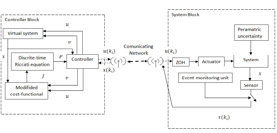
Figure 1: Block diagram of proposed robust control law using unrealiable communication channel.

It has three primary parts namely, system block , controller block and a unreliable communicating network between system and controller. The states of system are periodically measured by the sensor which is collocated with the system. The sensor is connected with the controller through a communication network. An event-monitoring unit verifies a state-dependent event condition periodically and transmits state information to the controller only when the event-condition is satisfied. The robust controller gain $K$ with eventual state information, $x(k_{i})$ which is received from uncertain system is used to generate the event-triggered control law $u(k_{i})=Kx(k_{i})$ to stabilize (5). Here $k_{i}$ denotes the latest event-triggering instant and the control input is updated at aperiodic discrete-time instant $k_{0},\ k_{1},\ k_{2}$. A zero-order-hold (ZOH) is used to hold the last transmitted control input until the next input is transmitted. Here the actuator is collocated with the system and actuating control law is assumed to change instantly with the transmission of input. For simplicity, this paper does not consider any time-delay between sensing, computation and actuation instant. But in real-practice there must be some delay. This delay will effect the system analysis and as well as in event-condition.
A discrete-time linear uncertain system (5) with event-triggered input

$$u(k_{i})=Kx(k_{i}),\ \ \ k\in\ [k_{i},\ k_{i+1})$$ (19)

is written as

$$x(k+1)=(A+\Delta A)x(k)+Bu(k_{i})$$ (20)

From [5], this can be modelled as

$$x(k+1)=(A+\Delta A+BK)x(k)+BKe(k)$$ (21)

The variable $e(k)$ is named as measurement error. It is used to represent the eventual state information $x(k_{i})$ in the form

$$e(k)=x(k_{i})-x(k)\ \ \ k\in[k_{i},\ k_{i+1})$$ (22)

Problem Statement: Design a feedback control law to stabilize the uncertain discrete-time event-triggered system (20) such that the closed loop system is ISS with respect to its measurement error $e(k)$.
Proposed solution:  This problem is solved in two different steps. Firstly, the controller is designed by adopting the optimal control and secondly an event-triggering rule is derived to make (20) ISS. The design procedure of controller gains, based on Theorems 1, is already discussed in Section II. The event-triggering law is derived from the Definition 1 & 2 assuming an ISS Lyapunov function $V(x)=x^{T}Px$. The design procedure of event-triggering condition is discussed elaborately in Section III.

III Main theoretical Results

This section discusses the design procedure of event-triggering condition and stability proof of (20) under presence of bounded parametric uncertainty. The results are stated in the form of a theorem.

Theorem 2.

Let $P>0$ be a solution of the Riccati equation (1) for a scalar $\epsilon>0$ and satisfy the following inequalities

$$Z=\epsilon^{-1}I+P(\epsilon^{-1}I-P)^{-1}P>0$$ (23)

$$\Delta A^{T}Z\Delta A\leq F$$ (24)

$$\beta^{2}I+K^{T}R_{1}K+L^{T}R_{2}L-A_{c}^{T}ZA_{c}\geq 0$$ (25)

where controller gains $K$ and $L$ are computed by (16), (17). The event-triggered control law (19) ensures the ISS of (20) $\forall p\in\Omega$ if the input is updated through the following triggering-condition

$$\left\lVert e(k)\right\rVert^{2}\geq\mu_{1}\left\lVert x(k)\right\rVert^{2}.$$ (26)

Moreover the design parameter $\mu_{1}$ is explicitly defined as

$$\mu_{1}=\frac{\sigma\lambda_{min}(Q_{1})}{\left\lVert K^{T}B^{T}ZBK\right\rVert}$$ (27)

where scalar $\sigma\ \in(0,1)$ and positive matrix $Q_{1}=(\beta^{2}I+K^{T}R_{1}K+L^{T}R_{2}L-A_{c}^{T}ZA_{c})$.

To prove the above theorem some intermediate results are stated in the form of following lemmas. The proof of these lemmas are omitted due to limitation of pages.

Lemma 1.

Let $P$ be a positive definite solution of (1). Then there exist a scalar $\epsilon>0$ such that

$$A_{c}^{T}P\Delta A+\Delta A^{T}PA_{c}+\Delta A^{T}P\Delta A\leq$$

$$A_{c}^{T}P(\epsilon^{-1}I-P)^{-1}PA_{c}+\epsilon^{-1}\Delta A^{T}\Delta A$$ (28)

with

$$(\epsilon^{-1}I-P)^{-1}>0$$ (29)

Lemma 2.

Let $P>0$ be a solution of (1) which satisfy the equation (23). Using controller gain (16) and (17), the following inequality holds

$$A_{c}^{T}ZA_{c}-A^{T}\big{\{}P^{-1}+BR_{1}^{-1}B^{T}+\alpha^{2}(I-BB^{+})$$

$$R_{2}^{-1}(I-BB^{+})^{T}\big{\}}^{-1}A\leq A_{c}^{T}(P^{-1}-\epsilon I)^{-1})A_{c}$$

$$-(L^{T}R_{2}L+K^{T}R_{1}K)$$ (30)

Proof of Theorem 2.

Assuming $V(x)$ as a ISS Lyapunov function for (20) and $A_{c}=(A+BK)$. The time difference of $V(x)$ $[\Delta V=V(x(k+1)-V(x(k))]$ along the direction of state trajectory of (20)  $\forall\ p\in\Omega$ is simplified Using Lemma (1).

$$\Delta V \leq x^{T}[\epsilon^{-1}A_{c}^{T}A_{c}+A_{c}^{T}P(\epsilon^{-1}I-P)^{-1}PA_{c}-P]x$$ (31)

$$+x^{T}[\Delta A^{T}P(\epsilon^{-1}I-P)^{-1}P\Delta A+\epsilon^{-1}\Delta A^{T}\Delta A]x$$

$$+e^{T}(\epsilon^{-1}K^{T}B^{T}BK+K^{T}B^{T}P(\epsilon^{-1}I-$$

$$P)^{-1}PBK)e$$

For further simplification, the solution of Riccati equation (1) $P$ is used in (31) to derive the following inequality

$$\Delta V \leq x^{T}A_{c}^{T}ZA_{c}x-x^{T}A^{T}\{P(k+1)^{-1}+$$ (32)

$$BR_{1}^{-1}B^{T}+\alpha^{2}(I-BB^{+})R_{2}^{-1}(I-$$

$$BB^{+})^{T}\}^{-1}Ax-x^{T}(Q+\beta^{2}I)x-x^{T}(F$$

$$-\Delta A^{T}Z\Delta A)x+e^{T}(K^{T}B^{T}ZBK)e$$

where $Z$ is defined in (1). Using Lemma 2, (32) is simplified as

$$\Delta V \leq -x^{T}(\beta^{2}I+K^{T}R_{1}K+L^{T}R_{2}L-A_{c}^{T}ZA_{c})x$$ (33)

$$+e^{T}K^{T}B^{T}ZBKe$$

Applying Definition 2 in (33), the system (20) remains ISS stable if error $e(k)$ satisfies the following inequality

$$\left\lVert e\right\rVert^{2}\geq\mu_{1}\left\lVert x\right\rVert^{2}$$ (34)

where parameter

$$\mu_{1}=\frac{\sigma\lambda_{min}(Q_{1})}{\left\lVert K^{T}B^{T}ZBK\right\rVert}.$$ (35)

The designed parameter $\sigma\in(0,1)$ and matrix $Q_{1}=(\beta^{2}I+K^{T}R_{1}K+L^{T}R_{2}L-A_{c}^{T}ZA_{c})>0$. The equation (34) represents the event-triggering law for (20). ∎

The proposed robust control framework considers the general system uncertainty, which includes both matched and mismatched component. Without mismatched part, system (5) reduces to matched system (defined in (6)), i.e. $\Delta A=B\phi(p)$ where $\phi(p)=B^{+}\{A(p)-A(p_{0})\}$ . Moreover, due to the absence of mismatched part, the virtual control input is not necessary in (11). As a special case of Theorem 1, the Corollary 1 is introduced for matched system.

Corollary 1.

Suppose there exist a scalar $\epsilon>0$ and a positive definite solution $P$ of Riccati equation

$$A^{T}\big{\{}P^{-1}+BR_{1}^{-1}B^{T})\big{\}}^{-1}A-P+Q+F+\beta^{2}I=0$$ (36)

with following conditions

$$\frac{2}{\epsilon}\phi^{T}B^{T}B\phi \leq F$$ (37)

$$(\epsilon^{-1}I-P)^{-1} > 0$$ (38)

Then $\forall p\in\Omega$, there exist a controller gain

$$K = -R_{1}^{-1}B^{T}\big{\{}P^{-1}+BR_{1}^{-1}B^{T}\big{\}}^{-1}A$$ (39)

which ensures the ISS of (5) through the event-triggered control law

$$\|e\|^{2}\geq\mu_{2}\|x\|^{2}$$ (40)

if the following sufficient condition holds

$$(\beta^{2}I+K^{T}R_{1}K-\frac{2}{\epsilon}A_{c}^{T}A_{c})\geq 0.$$ (41)

The parameter $\mu_{2}$ is derived as

$$\mu_{2}=\frac{\sigma\lambda_{min}(\tilde{Q})}{\|K^{T}B^{T}(P^{-1}-\epsilon I)^{-1}BK\|}$$ (42)

where scalar $\sigma\in(0,1)$ and $\tilde{Q}=Q+F+\beta^{2}I$.

Remark 2.

The event-triggering law (34) for (20) is designed. The designed parameter $\mu_{1}$ depends on the virtual gain $L$. Therefore $L$ has direct influence to design the robust stabilizing controller gain $K$ as well as on event-triggering law. The selection of design parameter $\beta$ and $\epsilon$ in (12) has a greater significance on system stability due to the fact that the positive definiteness of (18) depends on these parameters.

Remark 3.

Proposed framework can be extended in the presence of both system and input uncertainties and described by

$$x(k+1)=\big{[}A+\Delta A(p)\big{]}x(k)+\big{[}B+\Delta B(p)\big{]}u(k)$$ (43)

with a virtual dynamics (11) and a cost-functional

$$J = \frac{1}{2}\bigg{\{}\sum_{k=0}^{\infty}x(k)^{T}Qx(k)+x(k)^{T}Fx(k)+x(k)^{T}Hx(k)+$$ (44)

$$\beta^{2}x(k)^{T}x(k)+u(k)^{T}R_{1}u(k)+v(k)^{T}R_{2}v(k)\bigg{\}}$$

where $\beta>0$ and $H$ is a bound on $\Delta B$.

Comparison with existing results

This subsection compares the main contribution of this paper with the results reported in [10]-[11]. To compare with [10], the mismatched part of uncertainty is neglected. The Riccati equation mentioned in [10] is similar to proposed Riccati equation (1) in the presence of matched uncertainty. The only difference is we have added a term $\beta^{2}x^{T}x$ in the cost-functional (1). Without this extra term the Riccati equation (1) and controller gain (16) reduce to similar form as mentioned in [10]. So the results of (5) can be recovered as a special case of proposed results.

Moreover in Theorem $1$ of [10]-[11], an event-triggering condition is stated for matched system which depends on uncertain matrix $\phi(p)$. Implementation of this event-triggering condition is not realistic as matrix $\phi(p)$ is unknown. However in this paper, the proposed event triggering condition discussed in Theorem 2 is independent of uncertainty $\phi(p)$. It directly depends on the controller gain $K$. Moreover the triggering condition for matched system is also independent of uncertain matrix explicitly as seen from (42). Thus, it is concluded that the proposed event-triggering condition is comparatively more general and easy to realize than [10]-[11].

IV Numerical Examples and comparative studies

Consider an uncertain discrete-time linear system (20) where $A+\Delta A=\begin{bmatrix}p&1+p\\ 1&0\end{bmatrix}$, $B=\begin{bmatrix}0\\ 1\end{bmatrix}$. Here the system is mismatched in nature and the results of [10]-[11] are not applicable. To solve (1), matrices $Q=I$, $R_{1}=I$, $R_{2}=I$, $F=\begin{bmatrix}6.09&6.09\\ 6.09&6.09\end{bmatrix}$ and $\alpha=10$ are selected. The design parameter $\epsilon=0.1$, $\beta=5$ , $\sigma=0.1$ and $\mu=0.29$ are used. To design event-triggering condition $\sigma=0.1$ and $\mu=0.29$ are used. The uncertain parameter $p$ varies from $0$ to $0.8$. The simulation is carried-out in MATLAB for $20$ intervals with a sampling interval $T=1$ sec. The controller gains $K$ and $L$ are computed using (16), (17) and their numerical values are $K=[-0.9687-0.0001]$ and $L=\begin{bmatrix}-0.0006&-0.1\\ 0&0\end{bmatrix}$.

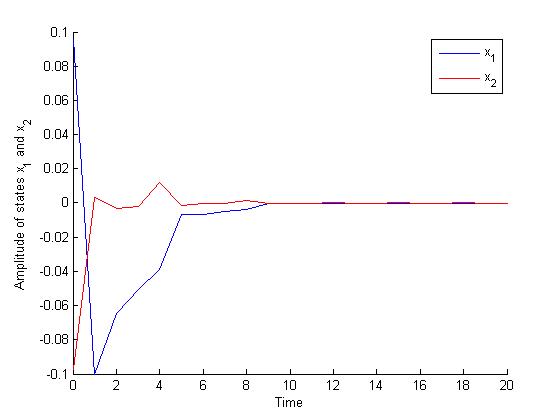
(a) Convergence of uncertain states for event-triggered control for $p=0.8$.

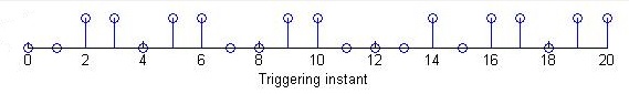
(b) Triggering instants at which control inputs are computed .

Figure 2: Results of periodic and event-triggered control.

Figure 2(a) shows the convergence of uncertain states for event-triggered control. For event triggered control the triggering instants are shown in Figure 2(b).

V Conclusion

A discrete-time periodic and aperiodic control of uncertain linear system is proposed in this paper. The control law is designed by formulating an optimal control problem for virtual nominal system with a modified cost-functional. An virtual input is defined to design the stabilizing controller gain along with the stability condition. The paper also proposes an event-triggered based control technique for NCS to achieve robustness. The event-condition and stability of uncertain system are derived using the ISS Lyapunov function. A new event-triggering law is derived which depends on the virtual controller gain in order to tackle mismatched uncertainty. A comparative study between existing and proposed results is also reported.

A challenging future work to extend the proposed robust control framework for discrete-time nonlinear system with and without event-triggering input. This frame work can be formulated as a differential game problem where the control inputs $u$ and $v$ can be treated as minimizing and maximizing inputs.

Appendix A

Proof of Theorem 1.

The proof has two parts. At first, we solve an optimal control problem to minimize (12) for the nominal system (11). For this purpose the optimal input $u$ and $v$ should minimize the Hamiltonian $H$, that means $\dfrac{\partial H}{\partial u}=0$ and $\dfrac{\partial H}{\partial v}=0$. After applying discrete-time LQR methods, the Riccati equation (1) and controller gains (16), (17) are achieved [22]. To prove the stability of uncertain system, let $V(x)=x(k)^{T}Px(k)$ be a Lyapunov function for (5). Then applying (20) the time difference of $V(x)$ along the $x$ is

$$\Delta V = x(k)^{T}A_{c}^{T}PA_{c}x(k)+x(k)^{T}A_{c}^{T}P\Delta Ax(k)$$ (45)

$$+x(k)^{T}\Delta APA_{c}x(k)+x(k)^{T}\Delta A^{T}P\Delta Ax(k)$$

$$-x(k)^{T}Px(k)$$

where $A_{c}=(A+BK)$. Using matrix inversion lemma, following is achieved [23]

$$(P^{-1}-\epsilon I)^{-1}=P+P(\epsilon^{-1}I-P)^{-1}P$$ (46)

Using (1) and (46) in (45), following is achieved

$$\Delta V \leq x(k)^{T}[A_{c}^{T}(P^{-1}-\epsilon I)^{-1}A_{c}-Q-\beta^{2}I-A^{T}\big{\{}P^{-1}$$ (47)

$$+BR_{1}^{-1}B^{T}+\alpha^{2}(I-BB^{+})R_{2}^{-1}(I-BB^{+})^{T}\big{\}}^{-1}$$

$$A]x(k)-x(k)^{T}[F-\epsilon^{-1}\Delta A^{T}\Delta A]x(k)$$

Now applying Lemmas 1, 2, the equation (47) is simplified as

$$\Delta V \leq -x(k)^{T}\big{\{}(\beta^{2}I+L^{T}R_{2}L+K^{T}R_{1}K)$$ (48)

$$-A_{c}^{T}(P^{-1}-\epsilon I)^{-1})A_{c}\big{\}}x(k)$$

The inequality (48) will be negative semi-definite if and only if equation (18) is satisfied. ∎

References

- [1] O. C. Imer and T. Basar,“Optimal control with limited controls”, American Control Conference, pp. 298-303, Minneapolis, 2006.
- [2] L. Zhang and D. H. Varsakelis, “LQG Control under Limited Communication”, 44th IEEE Conference on Decision and Control, pp. 185-190, Spain, 2005.
- [3] K. Astrom and B. Bernhardsson, “Comparison of Riemann and Lebesgue sampling for first order stochastic systems”, 41st IEEE Conference on Decision and Control, pp. 2011-2016, Las Vegas, 2002.
- [4] P. Tabuada, “Event-triggered real-time scheduling of stabilizing control tasks”, IEEE Transactions on Automatic Control, vol. 52(9), pp. 1680-1685, 2007.
- [5] A. Eqtami, D. V. Dimarogonas and K. J. Kyriakopoulos, “Event-triggered control for discrete-time systems”, American Control Conference, pp. 4719-4724, Baltimore, 2010.
- [6] A. Girard, “Dynamic Triggering Mechanisms for Event-Triggered Control”, IEEE Transactions on Automatic Control, vol. 60 no. 7, pp. 1992-1997, 2015.
- [7] N. Marchand, S. Durand, and J. F. G. Castellanos, “A General formula for event-based stabilization of nonlinear systems”, IEEE Transactions on Automatic Control, vol. 58(5), pp. 1332-1337, 2013.
- [8] A. Anta, and P. Tabuada, “To sample or not to sample:self-triggered control for nonlinear systems”. IEEE Transactions on Automatic Control, vol. 55(9), pp. 2030-2042, 2010.
- [9] X. Wang and M. D. Lemmon, “Self-triggered feedback control systems with finite-gain stability”, IEEE Transactions on Automatic Control, vol. 54(3), pp. 452-462, 2009.
- [10] E. Garcia, P. J. Antsaklis, “Optimal Model-Based Control with Limited Communication”, Proceedings of the 19th IFAC World, Cape Town, 2014.
- [11] E. Garcia, P. J. Antsaklis, L. A. Montestruque, “Model-Based Control of Networked Systems”, Springer, Switzerland, 2014.
- [12] K. Zhou, P. P. Khargonekar,“Robust stabilization of linear systems with norm-bounded time-varying uncertainty”, Systems & Control Letters, vol. 10, pp. 17-20, 1988.
- [13] I. R. Petersen and C. V. Hollt,“A Riccati Equation approach to the stabilization of uncertain linear systems”, Automatica, vol. 22, no. 4, pp. 397-411, 1986.
- [14] G. Garcia, J. Bernussou and D. Arzelier, “Robust stabilization of discrete-time linear systems with norm-bounded time varying uncertainty”, Systems & Control Letters, vol. 22, pp. 327-339, 1994.
- [15] W. P. M. H. Heemels, M. C. F. Donkers, A. R. Tell “Periodic event-triggered control for linear systems”, IEEE Transactions on Automatic Control, vol. 58(4), pp. 847-861, 2013.
- [16] W. P. M. H. Heemels, M. C. F. Donkers “Model-based periodic event-triggered control for linear systems”, Automatica, vol. 49, pp. 698-711, 2013.
- [17] A. Sahoo, H. Xu and S. Jagannathan,“Near optimal event-triggered control of nonlinear discrete-time systems using neurodynamic programming”, IEEE Transactions on Neural Networks and Learning Systems, (Early accesses), PP. 1-13, 2015.
- [18] S. Trimpe and R. DAndrea, “Event-based state estimation with variance-based triggering”, 51st IEEE Conference on Decision and Control, pp. 6583-6590, Hawaii, 2012.
- [19] P. Tallapragada and N. Chopra, “On event triggered tracking for nonlinear systems”, IEEE Transactions on Automatic Control, vol. 58(9), pp. 2343-2348, 2013.
- [20] E. D. Sontag, “Input to state stability: basic concepts and results”, Nonlinear and Optimal Control Theory, pp. 163-220, 2008.
- [21] D. Nesic and A.R. Teel, “Input-to-state stability of networked control systems”, Automatica, vol. 40(12), pp. 2121-2128, 2004.
- [22] D. S. Naidu, Optimal control systems, CRC press, India, 2009.
- [23] R. A. Horn and C. R. Johnson, Matrix Analysis, Cambridge University Press, Cambridge, 1990.
- [24] E. Garcia and P. J. Antsaklis, “Model-based event-triggered control for systems with quantization and time-varying network delays”, IEEE Transactions on Automatic Control, vol. 58(2), pp. 422-434, 2013.
- [25] F Lin. “An optimal control approach to robust control design”, International journal of control vol. 73(3), pp. 177-186, 2000.
- [26] F. Lin and R. D. Brandt, “An optimal control approach to robust control of robot manipulators”, IEEE Transactions on Robotics and Automation, vol. 14(1), pp. 69-77, 1998.
- [27] F. Lin, W. Zhang and R. D. Brandt,“Robust Hovering Control of a PVTOL Aircraft", IEEE Transactions on Control System Technology, vol. 7(3), pp. 343-351, 1999.
- [28] D. M. Adhyaru, I.N. Kar and M. Gopal, “Fixed final time optimal control approach for bounded robust controller design using Hamilton Jacobi Bellman solution”, IET Control Theory and Applications. vol. 3(9), pp. 1183-1195, 2009.
- [29] D. M. Adhyaru, I. N. Kar and M. Gopal, “Bounded robust control of systems using neural network based HJB solution”, Neural Comput and Applic, vol. 20(1), pp. 91-103, 2011.
- [30] M. Xia, V. Gupta and P. J. Antsaklis. “Networked state estimation over a shared communication medium”, American Control Conference, pp. 4128-4133 , Washington, 2013.
- [31] W. Wu, S. Reimann, D. Gorges, and S. Liu, “ Suboptimal event-triggered control for time-delayed linear systems ”, IEEE Transactions on Automatic Control, vol. 60(5), pp. 1386-1391, 2015.
- [32] H. K. Khalil, Nonlinear Systems, Prentice Hall, 3rd Edition, New Jersey, 2002.
- [33] W. wu, S. Reimann, D. Gorges and S.Liu, “Event-triggered control for discrete-time linear systems subjected to bounded disturbance”, International Journal of Robust and Nonlinear Control, Wiley, 2015.