Abstract

The relativistic calculations of the electromagnetic form factors, static moments and lepton decay constant of the $\rho$-meson are given in the framework of the instant form of the relativistic quantum mechanics with different model wave functions. The modified impulse approximation (MIA) is used for the electroweak current operator. MIA provides Lorentz covariance and conservation law for current operators. The developed approach gives the nonzero quadrupole moment due to the relativistic Wigner spin rotation in the $S$-state of the quarks in $\rho$-meson.

1 Introduction

The study of the electromagnetic structure of the $\rho$- meson remains relevant for many years. Interest in the study of electroweak structure of the $\rho$- meson has risen again recently in connection with new experimental data for the corresponding leptonic decay constant: $f^{exp}_{\rho}=152\pm 8MeV$[1]. This result is very important $\rho$-meson is short-lived particle and the experimental information about its electroweak properties (electromagnetic form factors and related static moments, charge radii, etc.) is poorly enough. However, there are a large number of theoretical approaches and models for description of this meson [2, 3, 4, 5, 6, 7, 8].

In this paper the description of the electromagnetic static moments and lepton decay constant of the $\rho$-meson is presented. Our approach is based on the use of the instant form (IF) of relativistic quantum mechanics (RQM). The detailed description of RQM can be found in the review [9].

The basic point of our approach is the procedure of the construction of the electroweak current operator [10, 11]. This construction is from the general method of relativistic invariant parameterization of local operator matrix elements proposed in the Ref. [12].

In fact, this procedure is a realization of the Wigner–Eckart theorem for the Poincaré group and it enables one for given matrix element of arbitrary tensor dimension to separate the reduced matrix elements (form factors) that are invariant under the Poincaré group. The matrix element of a given operator is represented as a sum of terms, each one of them being a covariant part multiplied by an invariant part. In such a representation a covariant part describes transformation (geometrical) properties of the matrix element, while all the dynamical information on the transition is contained in the invariant part – reduced matrix elements or form factors.

In our approach some rather general problems arising in the constituent quark models have been solved. For example, our description of composite systems, in fact, solves the problem of construction of the electromagnetic current satisfying the conditions of Lorentz covariance and conservation law [10].

Our calculations of the electroweak characteristics of $\rho$-meson are performed in the well known impulse approximation (IA). It means that the electromagnetic current of a composite system is a sum of one–particle currents of the constituents. It is worth emphasizing that in our method this approximation does not violate the standard conditions for the current. This is a variant of the relativistic impulse approximation formulated in terms of reduced matrix elements – modified impulse approximation (MIA) (see, e.g., [10]).

Using different model wave functions of quark in meson we calculate the electromagnetic form factors, the static properties and the lepton decay constant of $\rho$-meson supposing quarks to be in the $S$-state of relative motion. It is interesting to mention that relativistic effects occur to produce a nonzero quadrupole moment and quadrupole form factor. It is well known that in the nonrelativistic case the non–zero quadrupole form factor is caused by the presence of the $D$- wave and is zero otherwise.

2 Integral representation for the $\rho$-meson electromagnetic form factors and leptonic decay constant

Let us consider the matrix element of the $\rho$-meson electromagnetic current. In our constituent quark model the $u$- and $\overline{d}$– quarks are in the $S$-state of relative motion, that is $l=l^{\prime}=$ 0, with following total spin and total angular momentum: $J=J^{\prime}=S=S^{\prime}=$1. This matrix element is given in the Ref. [11]:

$$\langle\vec{p}_{c}\,,m_{J\rho}|j_{\mu}(0)|\vec{p}_{\rho}\,^{\prime}\,,m^{\prime}_{J\rho}\rangle=\langle\,m_{J\rho}|\,D^{1}(p_{\rho}\,,p^{\prime}_{\rho})\,\sum_{i=1,3}\,\tilde{\cal F}\,^{i}_{\rho}(t)\,\tilde{A}^{i}_{\mu}\,|m^{\prime}_{J\rho}\rangle\;;$$ (1)

$$\tilde{\cal F}\,^{1}_{c}(t)=\tilde{f}^{\rho}_{10}+\tilde{f}^{\rho}_{12}\left\{[i{p_{\rho}}_{\nu}\,\Gamma^{\nu}(p^{\prime}_{\rho})]^{2}\right.\left.-\frac{1}{3}\,\hbox{Sp}[i{p_{\rho}}_{\nu}\,\Gamma^{\nu}(p^{\prime}_{\rho})]^{2}\right\}\frac{2}{\hbox{Sp}[{p_{\rho}}_{\nu}\,\Gamma^{\nu}(p^{\prime}_{\rho})]^{2}}\;,$$

$$\tilde{\cal F}\,^{3}_{\rho}(t)=\tilde{f}^{\rho}_{30}\;;$$ (2)

$$\tilde{A}^{1}_{\mu}=(p_{\rho}+p^{\prime}_{\rho})_{\mu}\;,\quad\tilde{A}^{3}_{\mu}=\frac{i}{M_{\rho}}\varepsilon_{\mu\nu\lambda\sigma}\,p_{\rho}^{\nu}\,p^{\prime}_{\rho}\,{}^{\lambda}\,\Gamma^{\sigma}(p^{\prime}_{\rho})\;.$$

here $p^{\prime}_{\rho},p_{\rho}$ are 4-momentum of $\rho$-meson in initial and final states, respectively, $m^{\prime}_{J\rho}\,,m_{J\rho}$ are projections of the total angular momenta, $D^{1}(p_{\rho}\,,\,p^{\prime}_{\rho})$ is matrix of Wigner rotation, $\Gamma^{\nu}(p^{\prime}_{\rho})$ is 4-vector of spin, $M_{\rho}$ is $\rho$-meson mass, $\tilde{f}^{\rho}_{10}\,,\,\tilde{f}^{\rho}_{12}\,,$ $\tilde{f}^{\rho}_{30}$ are charge, quadrupole and magnetic form factors of $\rho$-meson, respectively.

The integral representations for the composite system form factors in (1), and (2) are obtained in the Refs. [10, 11]:

$$\tilde{f}^{\rho}_{in}(Q^{2})=\int\,d\sqrt{s}\,d\sqrt{s^{\prime}}\,\varphi(s)\,\tilde{G}_{in}(s,Q^{2},s^{\prime})\varphi(s^{\prime})\;,$$ (3)

here $\varphi(s)$ is wave function of quarks in RQM, $\tilde{G}_{in}(s,Q^{2},s^{\prime})$ is Lorentz-covariant generalized function (reduced matrix element on the Poincaré group).

Our form factors in (2) can be written in terms of conventional Sachs form factors for the system with the total angular momentum equal 1. To do this let us write the parameterization of the electromagnetic current matrix element in the Breit frame (see, e.g. [13]):

$$\langle\vec{p}_{\rho}\,,m_{J}|j_{\mu}(0)|\vec{p}_{\rho}\,^{\prime}\,,m^{\prime}_{J}\rangle=G^{\mu}(Q^{2})\;,$$

$$G^{0}(Q^{2})=2p_{\rho 0}\left\{(\vec{\xi}\,^{\prime}\vec{\xi}\,^{*})\,G_{C}(Q^{2})+\left[(\vec{\xi}\,^{*}\vec{Q})(\vec{\xi}\,^{\prime}\vec{Q})-\frac{1}{3}Q^{2}(\vec{\xi}\,^{\prime}\vec{\xi}\,^{*})\right]\,\frac{G_{Q}(Q^{2})}{2M_{\rho}^{2}}\right\}\;,$$

$$\vec{G}(Q^{2})=\frac{p_{\rho 0}}{M_{\rho}}\left[\vec{\xi}^{\prime}\,(\vec{\xi}\,^{*}\vec{Q})-\vec{\xi}\,^{*}(\vec{\xi}\,^{\prime}\vec{Q})\right]\,G_{M}(Q^{2})\;.$$ (4)

Here $G_{C}\;,\;G_{Q}\;,\;G_{M}$ are the charge, quadrupole and magnetic form factors, respectively.

The polarization vector in the Breit frame has the following form:

$$\xi^{\mu}(\pm 1)=\frac{1}{\sqrt{2}}(0\;,\;\mp 1\;,\;-\,i\;,\;0)\;,\quad\xi^{\mu}(0)=(0\;,\;0\;,\;0\;,\;1)\;.$$ (5)

The variables in $\xi$ are total angular momentum projections.

In the Breit frame:

$$q^{\mu}=(p_{\rho}-p^{\prime}_{\rho})^{\mu}=(0\;,\;\vec{Q})\;,\quad p_{\rho}^{\mu}=(p_{\rho 0}\;,\;\frac{1}{2}\vec{Q})\;,\quad p^{\prime}_{\rho}\,{}^{\mu}=(p_{\rho 0}\;,\;-\frac{1}{2}\vec{Q})\;,$$ (6)

$$p_{\rho 0}=\sqrt{M_{\rho}^{2}+\frac{1}{4}Q^{2}}\;,\quad\vec{Q}=(0\;,\;0\;,\;Q)\;.$$

Comparing (1) and (4) and taking into account the fact that in the Breit system $D^{1}_{m_{J}\,m^{\prime\prime}_{J}}(p_{\rho}\,,p_{\rho}^{\prime})=\delta_{m_{J}\,m^{\prime\prime}_{J}}\;,$ we have:

$$G_{C}(Q^{2})=\tilde{f}^{\rho}_{10}(Q^{2})\;,\quad G_{Q}(Q^{2})=\frac{2\,M_{\rho}^{2}}{Q^{2}}\,\tilde{f}^{\rho}_{12}(Q^{2})\;,$$

$$\quad G_{M}(Q^{2})=-\,M_{\rho}\,\tilde{f}^{\rho}_{30}(Q^{2})\;.$$ (7)

Let us use for (3) the modified impulse approximation formulated in terms of form factors $\tilde{G}_{iq}(s,Q^{2},s^{\prime})$. The physical meaning of this approximation is considered in detail in Ref. [10]. In the frame of MIA the invariant form factors $\tilde{G}_{iq}(s,Q^{2},s^{\prime})$ in (3) are changed by the so called free two–particle invariant form factors $g_{0i}(s,Q^{2},s^{\prime})\;(i=C,Q,M)$ describing the electromagnetic properties of the system of two free particles with the quantum numbers of the $\rho$-meson. So, the equations to be used for the calculation of the $\rho$–meson electromagnetic properties in MIA are the following:

$$G_{C}(Q^{2})=\int\,d\sqrt{s}\,d\sqrt{s^{\prime}}\,\varphi(s)\,g_{0C}(s\,,Q^{2}\,,s^{\prime})\,\varphi(s^{\prime})\;,$$

$$G_{Q}(Q^{2})=\frac{2\,M_{\rho}^{2}}{Q^{2}}\,\int\,d\sqrt{s}\,d\sqrt{s^{\prime}}\,\varphi(s)\,g_{0Q}(s\,,Q^{2}\,,s^{\prime})\,\varphi(s^{\prime})\;,$$ (8)

$$G_{M}(Q^{2})=-\,M_{\rho}\,\int\,d\sqrt{s}\,d\sqrt{s^{\prime}}\,\varphi(s)\,g_{0M}(s\,,Q^{2}\,,s^{\prime})\,\varphi(s^{\prime})\;.$$

The free two–particle invariant form factors can be calculated by the methods of relativistic kinematics and have the form given in Ref. [14].

For the calculation of the $\rho$-meson leptonic decay constants we used the method of parametrization matrix element of the current which is nondiagonal with respect to the total angular momentum [15].

Leptonic decay constant of the vector meson $f_{\rho}$ is determined by the following matrix element of the electroweak current (see, e.g. [17]):

$$\langle 0|j^{\rho}_{\mu}(0)|\vec{P_{\rho}},m_{\rho}\rangle=i\,\sqrt{2}f_{\rho}\,\xi_{\mu}(m_{\rho})\frac{1}{(2\pi)^{3/2}}\;,$$ (9)

In MIA the lepton decay constant of the $\rho$-meson is given by expression:

$$f_{\rho}=\int\,d\sqrt{s}\,G^{1,0,1}_{0,1}(s)\,\varphi(s)\;,$$ (10)

where the corresponding free form factor $G^{1,0,1}_{0,1}(s)$ is:

$$G^{1,0,1}_{0,1}(s)=-\frac{3\sqrt{3}(\sqrt{s}+2M)}{16\sqrt{s}\pi^{2}}\left(\frac{7s+12M\sqrt{s}+8M^{2}}{6s+12M\sqrt{s}+12M^{2}}\right)\;.$$ (11)

Thus an analytic expression for the constants can be represented as follows:

$$f_{\rho}=\frac{\sqrt{3}}{\pi\sqrt{2}}\int^{\infty}_{0}\,dk\,k^{2}\,\psi(k)\frac{(\sqrt{k^{2}+M^{2}}+M)}{(k^{2}+M^{2})^{3/4}}$$

$$\times\,\left(1+\frac{k^{2}}{3(\sqrt{k^{2}+M^{2}}+M)^{2}}\right)\;.$$ (12)

Note that an analytical expression for the $\rho$-meson leptonic decay constants obtained in our approach coincides with Refs. [16, 17].

3 The electromagnetic structure of the $\rho$-meson

In this section we make use of the results of the previous sections to calculate the $\rho$-meson electromagnetic properties.

The $\rho$-meson electromagnetic form factors are calculated using (8) in MIA. The wave functions in sense of RQM in (8) at $J=S=1\;,l=0$ are defined by the following expression (see, e.g. [10]):

$$\varphi(s)=\sqrt[4]{s}\,\psi(k)\,k\;,\quad k=\frac{1}{2}\sqrt{s-4\,M^{2}}\;,$$ (13)

and is normalized by the condition:

$$\int\,\psi^{2}(k)\,k^{2}\,dk=1\;,$$ (14)

here $\psi(k)$ is a model wave function.

For the description of the relative motion of quarks the following phenomenological wave functions are used:

1. A Gaussian or harmonic oscillator wave function (HO) (see, e.g. [18]):

$$\psi(k)=N_{HO}\,\hbox{exp}\left(-{k^{2}}/{2\,b^{2}}\right).$$ (15)

2. A power-law wave function (PL) (see, e.g. [18]):

$$\psi(k)=N_{PL}\,{(k^{2}/b^{2}+1)^{-n}}\;,\quad n=2\;,3\;.$$ (16)

For Sachs form factors of quarks we have:

$$G^{q}_{E}(Q^{2})=e_{q}\,f_{q}(Q^{2})\;,\quad G^{q}_{M}(Q^{2})=(e_{q}+\kappa_{q})\,f_{q}(Q^{2})\;,$$ (17)

where $e_{q}$ is the quark charge and $\kappa_{q}$ is the quark anomalous magnetic moment. For $f_{q}(Q^{2})$ the form proposed in Ref. [19] is used:

$$f_{q}(Q^{2})=\frac{1}{1+\ln(1+\langle r^{2}_{q}\rangle Q^{2}/6)}\;.$$ (18)

Here $\langle r^{2}_{q}\rangle$ is the mean square radius (MSR) of constituent quark.

The reasons of the choice for the function $f_{q}(Q^{2})$ can be found in Ref. [19] (see also Ref.[10]) The form (18) is based on the fact that this expression gives the asymptotics of the pion form factor at $Q^{2}\to\infty$ which coincides with the QCD prediction (see, e.g.[20]).

So, for the calculations we use a conventional set of parameters of constituent quark model. The structure of the constituent quark is described by the following parameters: $M_{u}=M_{\overline{d}}=M$ is the constituent quark mass, $\kappa_{u}\;,\;\kappa_{\overline{d}}$ are the constituent quarks anomalous magnetic moments, $\langle\,r^{2}_{u}\rangle=\langle\,r^{2}_{\overline{d}}\rangle=\langle\,r^{2}_{q}\rangle$ is the quark MSR. The interaction of quarks in $\rho$ meson is characterized by wave functions (15) – (16) with the parameters $b$.

Since the quark composition of the pion and $\rho$-meson are the same, then the parameters were fixed in our calculation as follows (see Ref.[21]).

1. We use $M$=0.22 GeV for the quark mass; the quark anomalous magnetic moments enter the our expressios through the sum ($\kappa_{u}+\kappa_{\overline{d}}$) and we take $\kappa_{u}+\kappa_{\overline{d}}$ = 0.0268 in natural units; for the quark MSR we use the relation $\langle r^{2}_{q}\rangle\simeq 0.3/M^{2}$.

2. The parameter of the wave function $b$ was fixed from the requirements of the description of experimental values of $\rho$-meson leptonic decay constants and following relation for the $\rho$-meson MSR from refs. [22, 23]:

$$\langle r^{2}_{\rho}\rangle-\langle r^{2}_{\pi}\rangle=0.11\pm 0.06fm^{2}\;.$$ (19)

For the pion MSR the experimental data is taken from Ref. [1]: $\langle r^{2}_{\pi}\rangle^{1/2}$ = 0.672$\pm$0.008 fm.

The $\rho$-meson MSR is calculated from relation:

$$\langle\,r^{2}_{\rho}\rangle=-6\,G^{\prime}_{C}(0)\;.$$ (20)

The $\rho$-meson mass in (8) is taken from Ref. [1]: $M_{\rho}$ = 775.5$\pm$0.4 MeV.

The magnetic $\mu_{\rho}$ and the quadrupole $Q_{\rho}$ moments of $\rho$ meson were calculated using the relations given in Ref. [13]:

$$G_{M}(0)=\frac{M_{\rho}}{M}\,\mu_{\rho}\;,\quad G_{Q}(0)=M_{\rho}^{2}\,Q_{\rho}\;.$$ (21)

The static limit in (8) gives the following relativistic expressions for moments:

$$\mu_{\rho}=\frac{1}{2}\,\int_{2M}^{\infty}\,d\sqrt{s}\,\frac{\varphi^{2}(s)}{\sqrt{s-4\,M^{2}}}\,\left\{1-L(s)+(\kappa_{u}+\kappa_{\overline{d}})\left[1-\frac{1}{2}\,L(s)\right]\right\}\;,$$ (22)

$$Q_{\rho}=-\,\int_{2M}^{\infty}\,d\sqrt{s}\,\frac{\varphi^{2}(s)}{\sqrt{s}}\,\left[\frac{M}{\sqrt{s}+2\,M}+\kappa_{u}+\kappa_{\overline{d}}\right]\,\frac{L(s)}{4M\sqrt{s-4M^{2}}}\;,$$ (23)

$$L(s)=\frac{2\,M^{2}}{\sqrt{s-4\,M^{2}}\,(\sqrt{s}+2\,M)}\,\left[\frac{1}{2\,M^{2}}\sqrt{s\,(s-4\,M^{2})}+\right.$$

$$+\left.\ln\,\frac{\sqrt{s}-\sqrt{s-4\,M^{2}}}{\sqrt{s}+\sqrt{s-4\,M^{2}}}\right]\;.$$

Let us note that the nonzero $\rho$-meson quadrupole moment appears due to the relativistic effect of Wigner spin rotation of quarks only. So, measuring of this quadrupole moment can be a test of the relativistic invariance in the confinement region.

Table 1: The $\rho$-meson electromagnetic moments and lepton decay constant obtained with the different model wave functions (15) – (16). $\langle\,r^{2}_{\rho}\rangle$ is MSR in $fm^{2}$, $\mu_{\rho}$ is relativistic magnetic moment (22) in natural units, $Q_{\rho}$ is quadrupole moment (23) in fm². The parameters $b$ in (15) and (16) are in $GeV$, $f_{\rho}$ is $\rho$-meson leptonic decay constant in $MeV$.

Wave
functions	$b\;$	$\langle\,r_{\rho}^{2}\rangle$	$\mu_{\rho}$	$Q_{\rho}$	$f_{\rho}$
(15)	0.228	0.597	2.01	-0.0064	152.2
(16) n=2	0.217	0.579	2.12	-0.0064	153.6
(16) n=3	0.379	0.560	2.16	-0.0066	154.9

The results of calculations for the $\rho$-meson electromagnetic form factors are represented in Fig.1–3.

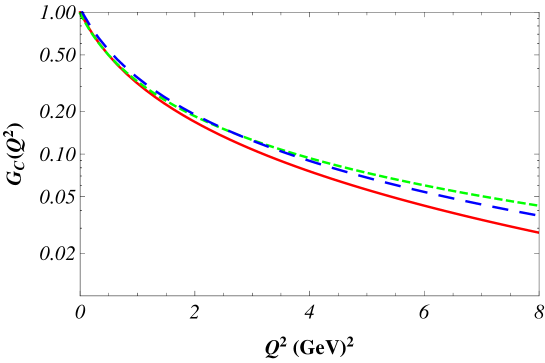
Figure 1: The results of the calculations of the $\rho$-meson charge form factor with different model wave functions. The values of the parameters are given in the Table 1. The solid line represents the relativistic calculation with the wave function (15), the short-dashed line – with (16) for $n=$ 2, the long-dashed line – with (16) for $n=$ 3.

Figure 2: The results of the calculations of the $\rho$-meson quadrupole form factor with different model wave functions, legend as in Figure 1

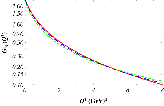
Figure 3: The results of the calculations of the $\rho$-meson magnetic form factor with different model wave functions, legend as in Figure 1.

4 Conclusion

The electromagnetic form factors, quadrupole and magnetic moments, MSR, and lepton decay constant of the $\rho$-meson were calculated in the framework of the instant form of relativistic quantum mechanic (RQM).

The special method of construction of the electromagnetic current matrix elements for the relativistic two–particle composite systems with nonzero total angular momentum is used to obtain the integral representation for the electromagnetic form factors and lepton decay constant.

The modified impulse approximation (MIA) is formulated in terms of reduced matrix elements on Poincaré group. MIA conserves Lorentz covariance of electroweak current and the electromagnetic current conservation law.

A reasonable description of the electromagnetic static moments and form factors and lepton decay constant of $\rho$-meson is obtained in the developed formalism. Our approach gives the nonzero quadrupole moment due to the relativistic Wigner spin rotation in the $S$-state of the two quarks in $\rho$-meson.

So, it is shown that developed variant of the the instant form of RQM can be used to obtain an adequate description of the electroweak properties of composite systems with nonzero total angular momentum.

References

• [1] K.A.Olive et.al. (Particlre Data Group), Chin. Phys. C 38, 090001 (2014).
• [2] Ho-Meoyng Choi, Chueng-Ryong Ji, Phys.Rev.D 70, 053015 (2004).
• [3] M.S. Bhagwat and P. Maris, Phys. Rev. C 77, 025203 (2008).
• [4] T.M. Aliver, A. Ozpineci, M. Saviei, Phys. lett. B 678, 470–476 (2009).
• [5] H.L.L. Roberts, A. Bashir, L.X. Gutierrez-Guerrero, C.D. Roberts and D.J. Wilson, Phys. Rev. C 83, 065206 (2011).
• [6] A.M. Badalin, Y. Simonov, Phys. Rev. D 87, 074012 (2013).
• [7] E.P. Bierrat, W. Schweiger, Phys. Rev. C 89, 055205 (2014).
• [8] C.S. Mello, A.N. da Silva, J.P.B.C. de Melo, T. Frederico, arXiv:1503.03398v2 [hep-ph], 1–6 (2015).
• [9] B.D. Keister and W. Polyzou, Adv. Nucl. Phys. 20, 225–479 (1991).
• [10] A.F. Krutov and V.E. Troitsky, Phys.Rev.C 65, 045501 (2002).
• [11] A.F. Krutov and V.E. Troitsky, Phys.Rev.C 68, 018501 (2003).
• [12] A.A. Cheshkov and Yu.M. Shirokov, Zh. Eksp. Teor. Fiz. 44, 1982–1992 (1963).
• [13] R.G. Arnold, C.E. Carlson, and F. Gross, Phys. Rev. C 21, 1426–1451 (1980).
• [14] A.F. Krutov, V.E. Troitsky, arXiv:0403046v1 [hep-ph], 1–16 (2003).
• [15] A.F. Krutov, R.G. Polezhaev, V.E. Troitsky, Theor. Math. Phys. 184:2, 1148–1162 (2015).
• [16] V.V. Andreev, arXiv:9912286v1[hep-ph], 1–6 (1999).
• [17] W. Jaus, Phys.Rev.D 67, 094010 (2003); arXiv:0212098v3[hep-ph](2003).
• [18] F. Coester and W.N. Polyzou, Phys. Rev. C 71, 028202 (2005).
• [19] A.F. Krutov and V.E. Troitsky, Teor. Mat. Fiz. 116, 215–224 (1998)[Theor. Math. Phys. 116:2, 907–913 (1998)].
• [20] V.A. Matveev, R.M. Muradyan, and A.N. Tavkhelidze, Lett. Nuovo Cim. 7, 719–723 (1973); S. Brodsky and G. Farrar, Phys. Rev. Lett. 31, 1153–1156 (1973).
• [21] A.F. Krutov and V.E. Troitsky, Eur. Phys. J. C 20, 71–76 (2001).
• [22] F. Cardarelli, I.L. Grach, I.M. Narodetskii, E. Pace, G. Salmé, and S. Simula, Phys. Rev. D 53, 6682–6685 (1996).
• [23] U. Vogl, M. Lutz, S. Klimt, and W. Weise, Nucl. Phys. A516, 469–495 (1990); B. Povh and J. Hüfner, Phys. Lett. B 245, 653–657 (1990); S.M. Troshin and N.E. Tyurin, Phys. Rev. D 49, 4427–4433 (1994).