Complete intersection for equivariant models

Abstract

Phylogenetic varieties related to equivariant substitution models have been studied largely in the last years. One of the main objectives has been finding a set of generators of the ideal of these varieties, but this has not yet been achieved in some cases (for example, for the general Markov model this involves the open “salmon conjecture”, see [2]) and it is not clear how to use all generators in practice. Motivated by applications in biology, we tackle the problem from another point of view. The elements of the ideal that could be useful for applications in phylogenetics only need to describe the variety around certain points of no evolution (see [13]). We produce a collection of explicit equations that describe the variety on a Zariski open neighborhood of these points (see Theorem 5.4). Namely, for any tree $T$ on any number of leaves (and any degrees at the interior nodes) and for any equivariant model on any set of states $\kappa$, we compute the codimension of the corresponding phylogenetic variety. We prove that this variety is smooth at general points of no evolution, and provide an algorithm to produce a complete intersection that describes the variety around these points.

1 Introduction

In the recent years there has been a huge amount of work done on phylogenetic varieties – we advise the reader to consult e.g. [4, 7, 12, 27, 39, 44] and references therein. These algebraic varieties contain the set of joint distributions at the leaves of a tree evolving under a Markov model of molecular evolution. From the biological point of view, these varieties are interesting because they provide new tools of non-parametric inference of phylogenetic trees. At present, the algebraic/geometric framework of phylogenetic varieties has allowed proving the identifiability of parameters of certain evolutionary models widely used by biologists [8, 3], proposing new methods of model selection [34], and producing new phylogenetic reconstruction methods [28, 15].

From the mathematical point of view, there has been a great effort in finding a whole description of the ideal of these phylogenetic varieties [6, 44, 24, 23]. Still, for some models, many questions remain open for trees on an arbitrary number of leaves $n$. Indeed, if one is interested in using these algebraic tools with real data, one would need a small set of generators of the ideal (rather than a description of the whole ideal); it would also be desirable to know the degree at which the ideal is generated [25, 40, 44]; and as the codimension of the variety is exponential in $n$, it is necessary to distinguish between generators that only account for the underlying evolutionary model, those that account for the tree topology, and those that could be useful for inferring the numerical parameters (see [7] for a good introduction to this topic).

For instance, the authors of [44] and [7] raised the question whether knowing complete intersection containing the phylogenetic variety and of the same dimension would be enough. Eminently, for biological applications it is only relevant to know the description of the variety around the points that make sense biologically speaking. If these points are smooth, then a complete intersection can define the variety on a neighborhood of these points.

This is the approach that was considered in [13, 32, 41] for the particular model of Kimura 3-parameter and is the same goal that we pursued in [18] for abelian group-based models. In the present paper we address this problem for the more general class of G-equivariant models, which contains more general algebraic models of interest to biologists (for example the strand-symmetric and the general Markov models). We give an explicit algorithm to construct a complete intersection that describes the variety on a dense open subset around a generic point of no evolution. Points of no evolution represent molecular sequences that remain invariant from the common ancestor to the leaves of the tree. Points in the phylogenetic variety that arise from biologically meaningful parameters are supposed to be near these points of no evolution (otherwise phylogenetic inference could not be made), and therefore it is important to study the variety around these points. Also, as we describe the variety at a dense open subset containing these points, we cover most (actually, all but possibly a subset of smaller dimension) of the biologically meaningful points of the variety. Also, in the same papers mentioned above, it is argued that a complete intersection can contain points in other irreducible components that can mislead the results in practice. However, the complete intersection we give contains a regular sequence of the edge invariants, which are known to be phylogenetic invariants [14]. Therefore, the other irreducible components of the complete intersection do not contain other phylogenetic varieties.

We prove first that these points are non-singular and therefore the variety can be described locally at these points by the smallest possible number of equations, the codimension of the variety. A system of generators of the local complete intersection can be explicitly computed. The degree of these generators is low and depends on a local description of claw trees related to the interior nodes of the tree and of the multiplicities of the permutation representation of the group $G\subset\mathfrak{S}_{\kappa}$. For example, for the biologically interesting models mentioned above, the complete intersection we provide has generators of degree at most 13. One should contrast this to the generators of the complete intersection given in [43] for the Kimura 3-parameter model, which had exponential degree in the number of leaves. Our approach is also useful in case one wants to use differential geometry for this variety (for example to compute the distance of a point to this variety, [26]).

The description of the ideal of phylogenetic invariants for $G$-equivariant models was provided by Draisma and Kuttler [24]. There are two ways to obtain the whole ideal of phylogenetic invariants for a given tree, assuming the ideals for star trees are known. The first description relies on the ideals of star trees associated to inner vertices of a given tree - so-called flattenings. The second description is inductive, where we regard a big tree as a join of two smaller trees.

Our approach is based on the second method. We start by inducing phylogenetic invariants from smaller trees. The induced phylogenetic invariants are of course not enough to provide a description for the larger tree. We complement them by so-called thin flattenings [14]. They are very explicit, however still numerous. It turns out that the choice of leaves in smaller trees distinguishes specific thin flattenings. Combining those with induced invariants yields our main result: under a minor assumption on claw trees (see 5.2) which is satisfied by the tripod on the most popular equivariant models (Jukes-Cantor, Kimura 3ST, strand symmetric) and also by the general Markov model, we provide an explicit local description of the variety associated to a model and a tree (see Theorem 5.4). Moreover, both in the starting point and in the induction process, the choices we make are almost canonical so that the complete intersection we produce is a natural one and could be reasonably used in practice.

The methods used in this paper rely on basic algebraic geometry and group representation theory. It is important to note that the results of the paper hold for any $G$-equivariant model, $G\subset\mathfrak{S}_{\kappa}$, for any $\kappa$, and therefore representation theory has been the necessary tool to deal with all these models at the same time. On the other hand, our results also hold for trees with any number of leaves and any degrees at the interior nodes.

The approach adopted to prove the main result 5.4 also produces a computationally effective list of elements in the ideal of the phylogenetic variety. Indeed, the list of equations provided in Theorem 5.4 for a tree $T$ with $n$ leaves is constructed from equations describing locally the phylogenetic varieties of claw trees of the interior nodes of $T$ and from certain minors of the thin flattenings mentioned above. The number of equations from the thin flattenings grows exponentially with $n$, but the number of equations corresponding to claw trees does not (it grows exponentially with the maximum degree of an interior node of $T$, see Remarks 4.7 and 5.6). However, evaluating the minors of the thin flattenings is not the optimal way of evaluating the rank of a matrix and these equations could therefore be substituted by a numerical method such as the singular value decomposition (see [28]). The remaining equations form a set that can be useful in practice, for example for the estimation of the parameters that maximize the likelihood via Lagrange multipliers (see the tools used in [22] and [21]).

The structure of the paper is as follows. In the following section 2, we recall the background on linear representation theory of finite groups that is needed in the sequel. In section 3, we recall the definition of equivariant models and of phylogenetic varieties. In this section we prove as well two key results that shall allow us to provide a complete intersection as desired: first we compute the dimension of the phylogenetic varieties for any equivariant model $\mathcal{M}_{G}$, $G\subset\mathfrak{S}_{\kappa}$, and any tree $T$, and then we prove that these varieties are smooth at generic points of no evolution. Then in section 4 we describe the set of equations that shall be used to prove our main result. The setup for this description is conceived towards the induction steps that are needed in the proof of the main result. In section 5 we describe the induction step and the “claw tree hypotheses” needed to prove our main result, Theorem 5.4 in the largest generality. The proof of this theorem is constructive and provides an algorithm for obtaining the desired complete intersection assuming the claw tree hypotheses is satisfied. In section 6 we prove that this claw tree hypothesis holds for trivalent trees on the general Markov model, the strand symmetric model, and the Jukes-Cantor model (the Kimura 3-parameter case was already considered in [13]). For these models we also specify complete intersections (following the algorithm provided in section 5) that describe the variety for quartet trees around generic points of no evolution.

2 Background on representation theory

In this section we recall the basic concepts of representation theory that will be needed in the sequel. The reader is referred to [42] or [31] for details and proofs. Throughout the paper we work over the field of complex numbers $\mathbb{C}$.

Let $G$ be a finite group. A representation of $G$ is a group homomorphism $\rho:G\rightarrow GL(V)$, where $V$ is a $\mathbb{C}$-vector space of finite dimension. We will refer to $V$ as the representation itself (or also as a $G$-module) if the map $\rho$ can be understood from the context, and for $g\in G$ and $u\in V$ we shall denote by $gu$ the vector $\rho(g)(u)$. A $G$-equivariant map is a linear map $f:V\longrightarrow V^{\prime}$ between two representations of $G$ that satisfies $f\circ\rho(g)=\rho_{V^{\prime}}(g)\circ f$ for all $g\in G$. The set of all $G$-equivariant maps between $V$ and $V^{\prime}$ is denoted as $\mathrm{Hom}\,_{G}(V,V^{\prime})$. Two $G$-modules $V$ and $V^{\prime}$ are said to be isomorphic (denoted as $V\cong_{G}V^{\prime}$) if there is a $G$-equivariant isomorphism of vector spaces $f:V\rightarrow V^{\prime}$. A representation $V$ is irreducible if it does not contain any proper $G$-invariant subspace. Otherwise, $V$ is said to be reducible. We will denote by $V^{G}$ the subspace of vectors of $V$ that are $G$-invariant under the action of $G$, that is, $gu=u$ for all $g\in G$.

Lemma 2.1 (Schur)

Let $V,V^{\prime}$ be two irreducible representations of $G$. If $f:V\rightarrow V^{\prime}$ is $G$-equivariant, then either $f=0$ or $f$ is an isomorphism, in which case ${\mathrm{Hom}\,_{G}(V,V^{\prime})\cong\mathbb{C}}$.

Notation 2.2

Let $\rho_{k}:G\rightarrow GL(N_{k})$, $k=1,\ldots,t$ be the irreducible representations of $G$ (up to isomorphism). We write $\chi_{k}$ for the character corresponding to $N_{k}$: $\chi_{k}(\sigma)=\operatorname{trace}(\rho_{k}(\sigma))$. We adopt the convention that $(\rho_{1},N_{1})$ refers to the identity (or trivial) representation.

Theorem 2.3 (Maschke)

If $\rho:G\rightarrow GL(V)$ is a representation of $G$, then there exists a unique decomposition $V=\oplus_{k=1}^{t}V[\chi_{k}]$, where each $V[\chi_{k}]$ is isomorphic to $\oplus^{m_{k}(V)}N_{k}$ for some multiplicity $m_{k}(V)\geq 0$. We call $V[\chi_{k}]$ the isotypic component of $V$ associated to $N_{k}$.

Notice that $V^{G}$ is equal to the isotypic component of $V$ associated to the trivial representation of $G$: $V^{G}=V[\chi_{1}]$.

Remark 2.4

By virtue of these fundamental results, for any representation $V$ of $G$, the dimension of $\mathrm{Hom}\,_{G}(N_{k},V)$ equals the multiplicity of $N_{k}$ in $V$. Moreover, the collection of the images of a chosen vector $v_{k}\in N_{k}$ under maps in $\mathrm{Hom}\,_{G}(N_{k},V)$ form a subspace $\mathcal{F}_{k}(V)$ in $V$ of dimension equal to the multiplicity of the isotypic component, $\mathcal{F}_{k}(V)\cong\mathbb{C}^{m_{k}(V)}$. Analogously to highest weight spaces, the spaces $\mathcal{F}_{k}(V)$ will represent the whole isotypic components. In particular, for any two representations $V,V^{\prime}$ we can identify $\mathrm{Hom}\,_{G}(V,V^{\prime})$ with $\bigoplus_{k}\mathrm{Hom}\,_{\mathbb{C}}(\mathcal{F}_{k}(V),\mathcal{F}_{k}(V^{\prime}))$.

Permutation representation.

From now on we focus on the following setting. Given a finite set $\Sigma$ of cardinality $\kappa$, we define $W=\langle\Sigma\rangle_{\mathbb{C}}$ as the $\mathbb{C}$-vector space generated by the elements of $\Sigma$. In this way, the elements of $\Sigma$ play the role of the standard basis of $W$, so that an element $\mathtt{X}\in\Sigma$ and the corresponding vector of the standard basis shall be denoted in the same way. Motivated by biology, in our examples we consider $\Sigma=\{\mathtt{A},\mathtt{C},\mathtt{G},\mathtt{T}\}$ but our work holds for any finite set. We denote $\mathbf{1}:=\sum_{\mathtt{X}\in\Sigma}\mathtt{X}$. By abuse of notation, $\mathbf{1}$ will be sometimes taken as the column-vector with all its $\kappa$ coordinates equal to one. Henceforth, $G$ shall be a permutation group of $\Sigma$, that is, $G$ is a subgroup of $\mathfrak{S}_{\kappa}$. The restriction to $G$ of the permutation representation $W$, given by the permutation of the elements in $\Sigma$, induces a representation $\rho(s)$ of $G$ on any tensor power $\otimes^{s}W$ by extending linearly the action $\sigma(\mathtt{X}_{i_{1}}\otimes\ldots\otimes\mathtt{X}_{i_{s}}):=\sigma\mathtt{X}_{i_{1}}\otimes\ldots\otimes\sigma\mathtt{X}_{i_{s}}$ for $\sigma\in G,\mathtt{X}_{i_{j}}\in\Sigma$. In this paper, we will only deal with such representations $\rho(s):G\longrightarrow GL(\otimes^{s}W)$ together with the irreducible representations $N_{1},\dots,N_{t}$ of $G$.

According to Masckhe’s theorem, any tensor power $\otimes^{s}W$ will decompose into a direct sum of modules $(\otimes^{s}W)[{\chi_{k}}]$ (the isotypic components) each of them being a number of copies of one of the irreducible modules $N_{k}$. This number is the multiplicity of $N_{k}$ in $\otimes^{s}W$ and will be denoted by $m_{k}(s)$. In the particular case $G=\mathfrak{S}_{k}$, explicit formulas for $m_{k}(s)$ can be provided in terms of Kronecker coefficients. We write $\mathbf{m}(s)=(m_{1}(s),\ldots,m_{t}(s))$ for the vector of multiplicities of $\otimes^{s}W$. As the case $s=1$ will play a special role, we simplify notation and write $\mathbf{m}=(m_{1},\ldots,m_{t})$ for the vector of multiplicities of $W$.

From now on, we fix subspaces $\mathcal{F}_{k}(W)\subset W$ for $k=1,\dots t$ according to Remark 2.4 by fixing a vector $v_{k}\in N_{k}$ and taking its images by maps in $\mathrm{Hom}\,_{G}(N_{k},W)$. This vector also defines subspaces $\mathcal{F}_{k}(\otimes^{s}{W})\subset\otimes^{s}W$, which shall be considered fixed from now on.

We consider the Hermitian inner product in $W$ that makes $\Sigma$ into an orthonormal basis, and denote it by $v\cdot w$ for any $v,w\in W$. This inner product will be used to identify $W$ with $W^{*}$ by sending a vector $v$ to the linear form $v^{*}\in W^{*}$ that maps $u$ to $v\cdot u$.

The inner product in $W$ induces an inner product in $\otimes^{s}W$ defined as

$$\mathtt{X}_{1}\otimes\ldots\otimes\mathtt{X}_{n}\cdot\mathtt{Y}_{1}\otimes\ldots\otimes\mathtt{Y}_{n}:=\prod_{k=1}^{s}\mathtt{X}_{k}\cdot\mathtt{Y}_{k},$$

for $\mathtt{X}_{i},\mathtt{Y}_{j}\in\Sigma$ and extending it sesquilinearly.

Dual representation.

If $\rho:G\longrightarrow GL(V)$ is a representation of $G$ with character $\chi$, then its dual $V^{*}$ is also a representation via the homomorphism $\rho^{*}:G\longrightarrow GL(V^{*})$ that maps $g$ to ${}^{t}\rho(g^{-1})$, and $V^{*}$ has character $\chi^{*}$ (the conjugate of $\chi$).

At the level of vector spaces, the inner product above provides an isomorphism $V\cong V^{*}$. Nevertheless, if $V$ is a representation of a group $G$, then it may happen that it is not $G$-isomorphic to $V^{*}$. This will force us to distinguish between the space and its dual in the sequel. However, the permutation representations $V=\otimes^{s}W$ that we consider in this paper satisfy $V\cong_{G}V^{*}$ because they have real characters. In particular, the $G$-isomorphism $V\cong_{G}V^{*}$ induces $G$-isomorphisms $V^{*}[\chi_{k}]\cong_{G}V[\chi_{k}]$ and $\mathcal{F}_{k}(V)\cong\mathcal{F}_{k}({V}^{*})$ for all $k$.

Thus, the reader may freely ignore all the dual signs in our article. We decided to keep them, as most of the arguments we provide hold without the assumption $V\cong_{G}V^{*}$ on a representation theoretic level. There is also a natural $G$-isomorphism $V\otimes V^{\prime}\cong_{G}\mathrm{Hom}\,(V^{*},V^{\prime})$ which at the level of $G$-invariant vectors translates to $\left(V\otimes V^{\prime}\right)^{G}\cong_{G}\mathrm{Hom}\,_{G}(V^{*},V^{\prime})$.

Representation theory allows us to decompose the ambient space $(\otimes^{n}W)^{G}$ in terms of the irreducible representations of $G$ as follows. This decomposition will be fundamental for us and will play a key role in the paper.

Proposition 2.5

For any $a+b=n$, there is a natural isomorphism of vector spaces

$$\left(\otimes^{a+b}W\right)^{G}\cong\bigoplus_{k=1}^{t}\;\mathcal{F}_{k^{*}}(\otimes^{a}W)\otimes\mathcal{F}_{k}(\otimes^{b}W).$$

In particular, the dimension of $(\otimes^{a+b}W)^{G}$ is $m_{1}(a+b)=\sum_{k=1}^{t}m_{k^{*}}(a)m_{k}(b)$, where $k^{*}$ is the index of the irreducible representation dual to $N_{k}$, that is, $N_{k^{*}}=(N_{k})^{*}$. Using the language of category theory, the functors $(\otimes^{n}\cdot)^{G}$ and $\bigotimes_{k=1}^{t}\mathcal{F}_{k^{*}}(\otimes^{a}\cdot)\otimes\mathcal{F}_{k}(\otimes^{b}\cdot)$ from the category of $G$ representations to the category of vector spaces are isomorphic.

Proof. Applying Maschke’s theorem and Schur’s lemma, we infer

$$(\otimes^{n}W)^{G} \cong \left((\otimes^{a}W)\otimes(\otimes^{b}W)\right)^{G}\cong\mathrm{Hom}\,_{G}((\otimes^{a}W)^{*},\otimes^{b}W)$$

$$\cong \oplus_{i,j}\mathrm{Hom}\,_{G}((\otimes^{a}W)^{*}[\chi_{i}],(\otimes^{b}W)[\chi_{j}])\cong\oplus_{k=1}^{t}\mathrm{Hom}\,_{\mathbb{C}}(\mathcal{F}_{k}(\otimes^{a}W^{*}),\mathcal{F}_{k}(\otimes^{b}W))$$

$$\cong \oplus_{k=1}^{t}\mathrm{Hom}\,_{\mathbb{C}}\left((\mathcal{F}_{k^{*}}(\otimes^{a}W))^{*},\mathcal{F}_{k}(\otimes^{b}W)\right)\cong\bigoplus_{k=1}^{t}\;\mathcal{F}_{k^{*}}(\otimes^{a}W)\otimes\mathcal{F}_{k}(\otimes^{b}W).$$

$\square$

3 Equivariant evolutionary models and phylogenetic varieties

A tree is a connected finite graph without cycles, consisting of vertices and edges. Given a tree $T$, we write $V(T)$ and $E(T)$ for the set of vertices and edges of $T$. The degree of a vertex is the number of edges incident to it. The set $V(T)$ splits into the set of leaves $L(T)$ (vertices of degree one) and the set of interior vertices $Int(T)$ : $V(T)=L(T)\cup Int(T)$. One says that a tree is trivalent if each vertex in $Int(T)$ has degree 3. A tree topology is the topological class of a tree where every leaf has been labeled. Given a subset $A$ of $L(T)$, the subtree induced by $A$ is just the smallest tree composed of the edges and vertices of $T$ in any path connecting two leaves in $A$. A tree $T$ is rooted if a specific node $r$ is labeled as the root.

In order to model the substitution of the states in $\Sigma$ according to a Markov process on a rooted tree $T$, one has to specify a distribution $\pi$ at the root of the tree and a collection of substitution matrices $\mathbf{A}=(A^{e})_{e\in E(T)}$ [19, 16]. The set of possible root distributions and substitution matrices for a tree $T$ is called the set of parameters. In the applications to biology, one has to restrict the set of parameters to stochastic vectors and matrices, but this restriction is unnecessary for the core of this paper. Below we describe equivariant models of evolution, which include some of the most well-known models.

As above, let $\Sigma$ be a finite set of cardinal $\kappa$, $W$ be the $\mathbb{C}$-vector space $\langle\Sigma\rangle_{\mathbb{C}}$, and $G\leq\mathfrak{S}_{\kappa}$ be a permutation group of $\Sigma$. In this section we use the distinguished basis $\Sigma$ of $W$ to identify $\kappa\times\kappa$ matrices with complex entries with $\mathrm{Hom}\,(W,W)$.

Definition 3.1

(cf. [24]) A rooted tree $T$ evolves under the equivariant model $\mathcal{M}_{G}$ if a $G$-invariant vector $\pi$ is associated to the root of $T$ and substitution matrices $A^{e}$ in $\mathrm{Hom}\,_{G}(W,W)$ are associated to each edge $e$ of $T$. For the equivariant model $\mathcal{M}_{G}$, the set of parameters is

$$\mathrm{Par}\,_{G}(T)=W^{G}\times\prod_{e\in E(T)}\mathrm{Hom}\,_{G}(W,W).$$

If one wants to talk about stochastic parameters, $s\mathrm{Par}\,_{G}(T)$ one has to restrict the root distribution to $sW^{G}:=W^{G}\cap\{\pi\in W\mid\pi\cdot\mathbf{1}=1\}$, and the substitution matrices to $s\mathrm{Hom}\,_{G}(W,W):=\mathrm{Hom}\,_{G}(W,W)\cap\{A\mid A\cdot\mathbf{1}=\mathbf{1}\}$ (and then require that all entries are real, nonnegative, but this is not relevant for our purposes). As a special case, if the group $G$ is trivial, $G=\{1\}$, we will denote by $\mathrm{Par}\,(T)$ and $s\mathrm{Par}\,(T)$ the corresponding spaces of parameters. The parametrization map that assigns a distribution at the leaves of $T$ to each set of parameters is

$$\Psi_{T}:\,\mathrm{Par}\,(T)\longrightarrow\otimes^{n}W$$ (1)

defined by

$$\Psi_{T}\left(\pi,\mathbf{A}\right)=\sum_{\mathtt{X}_{i}\in\Sigma}p_{\mathtt{X}_{1}...\mathtt{X}_{n}}\mathtt{X}_{1}\otimes\dots\otimes\mathtt{X}_{n},$$

where

$$p_{\mathtt{X}_{1}\dots\mathtt{X}_{n}}=\sum_{\mathtt{X}_{v}\in\Sigma,v\in Int(T)}\pi_{\mathtt{X}_{r}}\prod_{e\in E(T)}A^{e}_{\mathtt{X}_{pa(e)},\mathtt{X}_{ch(e)}}\,,$$ (2)

$\mathtt{X}_{v}$ denotes the state at the vertex $v$, $pa(e)$ (respectively $ch(e)$) is the parent (respectively, child) node of $e$, and $(\pi_{\mathtt{X}})_{\mathtt{X}\in\Sigma}$ are the coordinates of the root distribution $\pi$. When we restrict this map to the set of parameters $\mathrm{Par}\,_{G}(T)$, we denote it as $\Psi_{T}^{G}.$ In this case the image lies in $(\otimes^{n}W)^{G}$.

When the parametrization (1) is restricted to the set of stochastic parameters, we obtain

$$\phi_{T}:s\mathrm{Par}\,(T)\longrightarrow H\cap\otimes^{n}W,$$

where $H\subset\otimes^{n}W$ is the hyperplane defined as

$$H=\left\{p\in\otimes^{n}W\mid\sum_{\mathtt{X}_{i}\in\Sigma}p_{\mathtt{X}_{1}\dots\mathtt{X}_{n}}=1\right\}.$$

The analogous restrictions to $s\mathrm{Par}\,_{G}(T)$ are denoted as $\phi_{T}^{G}$. The word “stochastic” here has a broader meaning than usually, because for our aim we only need entries summing to one and not necessarily nonnegative entries.

The phylogenetic variety associated to a tree $T$ evolving under $\mathcal{M}_{G}$ is the (affine) algebraic variety

$$CV_{G}(T):=\overline{\{\Psi_{T}^{G}(\pi,\mathbf{A})\mid(\pi,\mathbf{A})\in\mathrm{Par}\,_{G}(T)\}}\subset(\otimes^{n}W)^{G}.$$

where $\overline{S}$ represents the Zariski closure of a set $S$. Similarly, the stochastic phylogenetic variety associated to a tree $T$ is the smallest algebraic variety $V_{G}(T)$ containing the set

$$\mathrm{Im}\,\,\phi_{T}^{G}=\left\{\phi_{T}^{G}(\pi,\mathbf{A}):(\pi,\mathbf{A})\in s\mathrm{Par}\,_{G}(T)\right\}.$$

One has $V_{G}(T)=CV_{G}(T)\cap H$ (see, for example, [16]). In particular, the equations defining $V_{G}(T)$ are the same equations defining $CV_{G}(T)$ plus the equation defining $H$.

Notice that in the definition of the phylogenetic variety we have not specified the root of the tree. It is well known that different root placements give rise to the same phylogenetic variety. Indeed, it is clear that a matrix $M$ belongs to $\mathrm{Hom}\,_{G}(W,W)$ if and only if so does its transpose $M^{t}$. Now, it can be seen that if we move the root from one node to a neighboring node and we replace the matrices $A^{e}$ of the edges with inverted orientation with their transpose, the image of the new parameters will remain the same. Moreover, we may assume that $\pi=\mathbf{1}$ when parameterizing $CV_{G}(T)$ since choosing an edge $e_{0}$ attached to the root and changing $A^{e_{0}}$ by $diag(\pi)A^{e_{0}}$ gives rise to the same image point. Hence $CV_{G}(T)$ does not depend on the root. As $H$ also does not depend on the root, neither does $V_{G}(T)$.

In case we take all matrices $A^{e}$ equal to the identity, the image by $\Psi_{T}^{G}$ represents no evolution at all.

Definition 3.2

Given an equivariant model $\mathcal{M}_{G}$, a point $\pi_{n}$ in $\otimes^{n}W$ is a point of no evolution if $\pi_{n}=\sum_{\mathtt{X}\in\Sigma}\pi_{\mathtt{X}}\mathtt{X}\otimes\ldots\otimes\mathtt{X}$ and $\pi_{n}$ is invariant under $G$.

If $\pi_{n}=\sum_{\mathtt{X}\in\Sigma}\pi_{\mathtt{X}}\mathtt{X}\otimes\ldots\otimes\mathtt{X}$ is a point of no evolution, then it belongs to $CV_{G}(T)$ for any tree $T$ on $n$ leaves because $\pi_{n}=\Psi_{T}^{G}(\pi,\mathbf{I})$ where $\pi=\sum_{\mathtt{X}\in\Sigma}\pi_{\mathtt{X}}\mathtt{X}\in W^{G}$ and $\mathbf{I}$ corresponds to the identity matrix at each edge: $\mathbf{I}=(Id)_{e\in E(T)}$.

Remark 3.3

For biological applications, we are interested in real/stochastic points in $\otimes^{n}W$ that are close to points of no evolution (in the complex euclidean distance). Indeed, as $\Psi_{T}^{G}$ is a continuous map, if $p$ is close to a point of no evolution $\pi_{n}$, then there is a preimage of $p$ close to $(\pi,\mathbf{I})$. The parameters close to $(\pi,\mathbf{I})$ are precisely those that are interesting biologically speaking because they account for probabilities of no mutation greater than probabilities of mutation (that is, diagonal entries greater than off-diagonal entries in transition matrices). To this end, the main goal of this paper is to provide a local description of the phylogenetic varieties around the points of no evolution.

Example 3.4

The definition of equivariant model includes important evolutionary models used in phylogenetics for $\kappa=4$ like

1. Jukes-Cantor [33], for $G=\mathfrak{S}_{4}$ or $G=\mathfrak{A}_{4}$ (the alternating group);

2. Kimura 2-parameter [35], for $G=\langle(\mathtt{A}\mathtt{C}\mathtt{G}\mathtt{T}),(\mathtt{A}\mathtt{G})\rangle$;

3. Kimura 3-parameter [36], for $G=\langle(\mathtt{A}\mathtt{C})(\mathtt{G}\mathtt{T}),(\mathtt{A}\mathtt{G})(\mathtt{C}\mathtt{T})\rangle$;

4. strand-symmetric [17], for $G=\langle(\mathtt{A}\mathtt{T})(\mathtt{C}\mathtt{G})\rangle$;

5. general Markov (briefly GMM) [10], for $G=\{1\}$.

We say that $\mathcal{M}_{G}$ is a submodel of $\mathcal{M}_{H}$ if $H\leq G$. With this terminology, all the models above are submodels of the general Markov model and we have inclusions from top to bottom on the sets of corresponding parameters (and algebraic varieties).

3.1 Dimension of phylogenetic varieties for equivariant models

In this subsection we compute the dimension of the phylogenetic variety associated to any $G$-equivariant model on any tree $T$, $G\leq\mathfrak{S}_{\kappa}$. This dimension was already known in the particular cases of the Jukes-Cantor, Kimura 2 and 3 parameters and general Markov model. The result yields the codimension of these varieties and hence it is the first step towards providing a complete intersection containing them.

Theorem 3.5

For any group $G\leq\mathfrak{S}_{\kappa}$ and any tree $T$ without nodes of degree 2, the dimension of $V_{G}(T)$ is $|E(T)|(m_{1}(2)-m_{1})+m_{1}-1$ and the dimension of $CV_{G}(T)$ is $|E(T)|(m_{1}(2)-m_{1})+m_{1}$.

Proof. The dimension of $V_{G}(T)$ is upper bounded by the dimension of $s\mathrm{Par}\,_{G}(T)$, which we compute in the following.
Each transition matrix $M$ is an element of

$$\mathrm{Hom}\,_{G}(W,W)\cong(W^{*}\otimes W)^{G},$$

so, as in our case $W\cong W^{*}$, the number of parameters is $m_{1}(2)$. However, because of the stochastic assumption, the sum of the rows of each matrix $M$ is fixed to one. Notice that $(W^{*}\otimes W)^{G}$ surjects onto $W^{G}$ by the map $M\mapsto M\mathbf{1}$. Hence, there are $m_{1}$ independent restrictions on the parameters of $M$. This makes $|E(T)|(m_{1}(2)-m_{1})$ free parameters for the choice of the transition matrices.
On the other hand, the distribution of the root is given by a vector $\pi\in W^{G}$. The stochastic condition implies that the sum of the coordinates is equal to one. This makes $m_{1}-1$ free parameters for the choice of the root distribution.
Summing up, we have that $\dim V_{G}(T)$ is less or equal than $|E(T)|(m_{1}(2)-m_{1})+(m_{1}-1)$.

In order to prove the other inequality we use Chang’s result ([19]) and its generalization ([4]) on the “generic identifiability of parameters“ of the general Markov model $\mathcal{M}_{1}$ on trees without nodes of degree 2. This result says that the fiber of $\phi_{T}(\mathcal{P})$ is finite for parameters $\mathcal{P}=\left(\pi,(A^{e})_{e}\right)$ that satisfy: (1) no entry of $\pi$ is zero; (2) all $A^{e}$ are non-singular; and (3) $\det A^{e}\neq\pm 1$ for all $e$. These generic conditions $(1)$-$(3)$ are also generic for the parameters of any equivariant model $\mathcal{M}_{G}$. That is, if $\Sigma=\{\mathtt{X}_{1},\dots,\mathtt{X}_{\kappa}\}$, for any group $G\leq\mathfrak{S}_{\kappa}$ we have

1. $sW^{G}$ is not included in $\{\pi\in W\,\mid\pi_{\mathtt{X}_{1}}\cdot\ldots\cdot\pi_{\mathtt{X}_{\kappa}}=0\}$ (indeed, $\frac{1}{\kappa}\mathbf{1}\in sW^{G}$ for example),

2. $s\mathrm{Hom}\,_{G}(W,W)$ is not contained in the set of singular matrices (indeed, $Id\in s\mathrm{Hom}\,_{G}(W,W)$), and

3. $s\mathrm{Hom}\,_{G}(W,W)$ does not only contain matrices with determinant $1$ or $-1$ (for example, the matrix with all entries equal to $1/{\kappa}$ belongs to $s\mathrm{Hom}\,_{G}(W,W)$).

This means that for generic parameters $\mathcal{P}\in s\mathrm{Par}\,_{G}(T)$, if we set $p=\phi_{T}^{G}(\mathcal{P})$, the preimage $(\phi_{T})^{-1}(p)$ is finite. As the preimage $(\phi_{T})^{-1}(p)$ contains $(\phi_{T}^{G})^{-1}(p)$, this implies that the generic fiber of $\phi_{T}^{G}$ is finite. Therefore, the dimension of $V_{G}(T)$ is upper bounded by the dimension of the domain of $\phi_{T}^{G}$, which has been computed above.

The claim for $CV_{G}(T)$ follows because it is the closure of the cone over $V_{G}(T)$. $\square$

This result implies the generic identifiability of the stochastic parameters for trees evolving under equivariant models (see [9, Definition 1] for example).

Corollary 3.6

The stochastic parameters of a tree $T$ evolving under an equivariant model $\mathcal{M}_{G}$, $G\leq\mathfrak{S}_{\kappa}$, are generically identifiable if $T$ has no nodes of degree 2.

Remark 3.7

It can be checked easily that for the evolutionary models listed in Example 3.4, the dimension for a trivalent tree on $n$ leaves (and hence with $2n-3$ edges) $T$ is

1. $\dim_{\mathbb{C}}V_{G}(T)=2n-3$ for the Jukes-Cantor model;

2. $\dim_{\mathbb{C}}V_{G}(T)=4n-6$ for the Kimura 2-parameter model;

3. $\dim_{\mathbb{C}}V_{G}(T)=6n-9$ for the Kimura 3-parameter model;

4. $\dim_{\mathbb{C}}V_{G}(T)=12n-17$ for the strand symmetric model;

5. $\dim_{\mathbb{C}}V_{G}(T)=24n-33$ for the general Markov model.

If $T$ has $n$ leaves, we will write $\mathrm{codim}\,(T)$ for the codimension of $CV_{G}(T)$ in $(\otimes^{n}W)^{G}$ (equal to the codimension of $V_{G}(T)$ in $H$), that is, $\mathrm{codim}\,(T):=\dim(\otimes^{n}W)^{G}-\dim CV_{G}(T)$. The dimension of $(\otimes^{n}W)^{G}$ is $m_{1}(n)$, which has been computed in [16, Prop. 20] for the models listed in Example 3.4.

3.2 Smoothness at points of no evolution

Let $T_{n}$ be the claw $n$-tree, that is, the tree with one inner vertex and $n$ leaves. In what follows we prove that the variety corresponding to $T_{n}$ is smooth at generic points of no evolution. In particular, it can be locally defined by a complete intersection.

Given a permutation subgroup $G$ of $\mathfrak{S}_{\kappa}$, we denote by $GL(\kappa)^{G}$ the group of $G$-equivariant $\kappa\times\kappa$ invertible matrices. Clearly, $GL(\kappa)^{G}$ defines an action on $\mathrm{Hom}\,_{G}(W,W)$ by $(A,M)\rightarrow AM$.

Theorem 3.8

The variety $CV_{G}(T_{n})$ is the Zariski closure of the orbit of $\Psi_{T}^{G}(\mathbf{1},\mathbf{I})$ under the group action of $(GL(\kappa)^{G})^{n}$.

Proof. The conditions

• $\det A^{e}\neq 0$ for all $e\in E(T)$, and

• all coordinates $\pi$ are different from $0$

define open sets in $\mathrm{Par}\,_{G}(T)$. As $\mathbf{I}\in GL(\kappa)^{G}$ and $\mathbf{1}\in W^{G}$, the intersection of these open sets is non-empty and a generic point $(\pi,A^{e})\in\mathrm{Par}\,_{G}(T)$ satisfies both conditions. Let us fix one edge $e_{0}$. Notice that $diag(\pi)A^{e_{0}}$ is invertible (as the coordinates of $\pi$ are nonzero) and is $G$-invariant (as $\pi\in V^{G}$). This means $diag(\pi)A^{e_{0}}\in GL(\kappa)^{G}$. Notice that $\Psi_{T}^{G}(\pi,A^{e})=\Psi_{T}^{G}(\mathbf{1},\tilde{A}^{e})$, where $\tilde{A}^{e}=A^{e}$ for $e\neq e_{0}$ and $\tilde{A}^{e_{0}}=diag(\pi)A^{e_{0}}$. However, $\Psi_{T}^{G}(\mathbf{1},\tilde{A}^{e})=(\tilde{A}^{e})\cdot\Psi_{T}^{G}(\mathbf{1},\mathbf{I})$. $\square$

Corollary 3.9

If $\sum_{\mathtt{X}\in\Sigma}\pi_{\mathtt{X}}\mathtt{X}\otimes\ldots\otimes\mathtt{X}$ satisfies $\pi_{\mathtt{X}}\neq 0$ for all $\mathtt{X}$, then it is nonsingular. In particular, a generic point of no evolution of $CV_{G}(T_{n})$ and $V_{G}(T_{n})$ is nonsingular.

Proof. For $CV_{G}(T_{n})$ the statement follows directly from Theorem 3.8. Let us also notice that $CV_{G}(T_{n})$ is a cone, hence a point of $V_{G}(T_{n})$ is smooth if and only if it is smooth as a point of $CV_{G}(T_{n})$. $\square$

Remark 3.10

When $G$ acts on the basis of $V$ transitively and freely then $GL(V)^{G}$ is a torus. This is the case of so-called group-based models and, as follows from Theorem 3.8 the variety $V_{G}(T_{n})$ is toric [44].

4 Equations for the complete intersection

A bipartition $A|B$ of the set of leaves is just a decomposition $L(T)=A\cup B$, where $A$ and $B$ are disjoint sets. Throughout the paper, we write $a=|A|$, $b=|B|$ and, to avoid trivialities, we will assume that $a,b\geq 2$. A bipartition is an edge split of $T$ if it arises by removing one of the edges of $T$. If $A\subset L(T)$, we denote $\otimes_{i\in A}W_{i}$ by $W_{A}$.

Given a tree $T$, in this section we proceed to construct equations that will define a complete intersection for $CV_{G}(T)$. We choose an internal edge $e$ of $T$, which induces an edge split of the set of leaves $L(T)=A\cup B$. This allows us to view the tree $T$ as the gluing of two trees $T=T_{A}*T_{B}$ where $L(T_{A})=A\cup L_{A}$, $L(T_{B})=B\cup L_{B}$, and $L_{A}$,$L_{B}$ are the two vertices of the edge $e$, see Figure 1 and [6]. We assume that the leaves of $T$ are ordered so that those in $A$ appear in the first place, and those in $B$ appear afterwards. We call $\alpha\in L(T_{A})$ the last leaf of $A$ and $\beta\in L(T_{B})$ the first leaf of $B$.

A complete intersection for the variety $CV_{G}(T)$ will be obtained by joining equations of a complete intersection for $CV_{G}(T_{A})$, of a complete intersection for $CV_{G}(T_{B})$ and specific edge invariants. All results of this section (and the following) still hold if we replace the vector $\mathbf{1}$ by any other $G$-invariant vector of $W$.

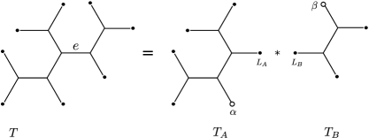
Figure 1: Decomposition of $T$ into two subtrees $T_{A}$, $T_{B}$: $T=T_{A}\ast T_{B}$.

4.1 A basis linked to an edge split

In order to provide specific equations for the varieties associated to phylogenetic trees, we proceed to construct a basis $\mathcal{B}_{A|B}$ of $(\otimes^{n}W)^{G}$ related to a given edge split $A|B$ as above. This basis shall be used to specify coordinates and provide the equations as polynomials in these specific indeterminates. The important point is that this basis must be consistent with the decomposition

$$(\otimes^{n}W)^{G}\cong\oplus_{k=1}^{t}\mathrm{Hom}\,_{\mathbb{C}}(\mathcal{F}_{k}(W_{A}^{*}),\mathcal{F}_{k}(W_{B})).$$ (3)

given by Proposition 2.5.

We construct the desired basis of $(\otimes^{n}W)^{G}$ compatible with (3) as follows.

Algorithm to construct a basis of $(\otimes^{n}W)^{G}$ linked to an edge split.

1. Choose bases $\{u^{k}_{i}\}_{i=1\div m_{k}}$ of each $\mathcal{F}_{k}(W)$, $k=1,\ldots,t$.

2. For each $k=1,\dots,t$, the vectors $u^{k}_{B,i}:=u^{k}_{i}\otimes\mathbf{1}^{b-1}$ of $\mathcal{F}_{k}(W_{B})$, $i=1\div m_{k}$, are linearly independent. Indeed, the monomorphism $W_{\beta}\stackrel{{\scriptstyle\cdot\otimes\mathbf{1}^{b-1}}}{{\longrightarrow}}W_{B}$ obtained by tensoring with a power of $\mathbf{1}$ induces a monomorphism $\mathcal{F}_{k}(W)\stackrel{{\scriptstyle\iota}}{{\hookrightarrow}}\mathcal{F}_{k}(W_{B})$. We extend them to a basis $\{u^{k}_{B,i}\}_{i=1\div m_{k}(b)}$ of $\mathcal{F}_{k}(W_{B})$.

3. We repeat step 2 for $A$ to obtain a basis $\{u^{k^{*}}_{A,i}\}_{i=1\div m_{k}(a)}$ of $\mathcal{F}_{k^{*}}(W_{A})$ for each $k$ (but now tensoring at the left, $\mathbf{1}^{a-1}\otimes u^{k^{*}}_{i}$).

4. Write $S$ for the inverse of the isomorphism of Proposition 2.5. Its restrictions induce natural isomorphisms from

   $$\mathcal{F}_{k^{*}}(W_{A})\otimes\mathcal{F}_{k}(W_{B})\cong\mathrm{Hom}\,_{\mathbb{C}}(\mathcal{F}_{k^{*}}(W_{A})^{*},\mathcal{F}_{k}(W_{B}))$$

   to

   $$\mathrm{Hom}\,_{G}(W_{A}^{*}[\chi_{k}],W_{B}[\chi_{k}])\cong(W_{A}[\chi_{k^{*}}]\otimes W_{B}[\chi_{k}])^{G}.$$

   We call $\mathcal{B}_{A|B}$ the desired basis $\{S(u^{k^{*}}_{A,i}\otimes u^{k}_{B,j})\}_{i,j,k}$ of $(\otimes^{n}W)^{G}$.

From now on, we will denote by $q^{k}_{ij}$ the coordinate corresponding to the basis vector $S(u^{k^{*}}_{A,i}\otimes u^{k}_{B,j})$.

Remark 4.1

We describe here the isomorphism $S$ mentioned above. Let $f$ be the morphism in $\mathrm{Hom}\,_{\mathbb{C}}((\mathcal{F}_{k^{*}}(W_{A})^{*},\mathcal{F}_{k}(W_{B}))$ corresponding to $u^{k^{*}}_{A,i}\otimes u^{k}_{B,j}$ (this is, $f(\omega)=\omega(u^{k^{*}}_{A,i})u^{k}_{B,j}$). To present $f$ as an element $S(f)\in\mathrm{Hom}\,_{G}(W_{A}^{*}[\chi_{k}],W_{B}[\chi_{k}])$ we proceed as follows:

1. Denote by $\{(u^{k^{*}}_{A,i})^{*}\}_{i}\subset\mathcal{F}_{k}(W_{A}^{*})$ the dual basis for $\{u^{k^{*}}_{A,i}\}_{i}$. Choose a subset $H\subset G$ such that, for any $i=1\div m_{k}(a)$, $\{h(u^{k^{*}}_{A,i})^{*}\}_{h\in H}$ is a basis of a subrepresentation in $W_{A}^{*}[\chi_{k}]$ (necessarily isomorphic to $N_{k}$).

2. Then, $\{h(u^{k^{*}}_{A,i})^{*}\}_{h\in H,i=1\div m_{k}(a)}$ is a basis of $W_{A}^{*}[\chi_{k}]$.

3. We define $S(f)(h(u^{k^{*}}_{A,i})^{*})=hu^{k}_{B,j}$ and $S(f)(h(u^{k^{*}}_{A,l})^{*})=0$ for $l\neq i$. This is the natural $G$-equivariant morphism associated to $f$.

The following statement claims that under stronger assumptions, the image of $S(u^{k^{*}}_{A,i}\otimes u^{k}_{B,j})$ under the canonical isomorphism $\mathrm{Hom}\,_{G}(W_{A}^{*}[\chi_{k}],W_{B}[\chi_{k}])\cong(W_{A}[\chi_{k^{*}}]\otimes W_{B}[\chi_{k}])^{G}$ has the particularly nice form of the averaging operator. Namely,

Lemma 4.2

If we can choose $H$ to be a subgroup of $G$, then

$$S(u^{k^{*}}_{A,i}\otimes u^{k}_{B,j})=\frac{n_{k}}{|G|}\sum_{g\in G}(gu^{k^{*}}_{A,i})\otimes(gu^{k}_{B,j}),$$

where $n_{k}$ is the cardinality of $H$ (equal to the dimension of $N_{k}$).

Proof. First we notice that the kernel of the averaging operator always contains the kernel of $S(u^{k^{*}}_{A,i}\otimes u^{k}_{B,j})$. Moreover, the result of the averaging operator is a $G$-equivariant homomorphism. It remains to evaluate it on $(u^{k^{*}}_{A,i})^{*}$. Notice that for each $h\in H$, we have $G=\{g^{-1}h:g\in G\}$. Hence we have the following equality

$$\sum_{g\in G}\left(u^{k}_{A,i}\right)^{*}\left(gu^{k^{*}}_{A,i}\right)\;gu^{k}_{B,j}=\sum_{g\in G}\left(u^{k}_{A,i}\right)^{*}\left(g^{-1}hu^{k^{*}}_{A,i}\right)\;g^{-1}hu^{k}_{B,j}.$$

Therefore, the right hand part of the equality in the lemma when evaluated at $(u^{k^{*}}_{A,i})^{*}$ is:

$$\frac{n_{k}}{|G|}\sum_{g\in G}\left(u^{k^{*}}_{A,i}\right)^{*}\left(gu^{k^{*}}_{A,i}\right)\;gu^{k}_{B,j} = \frac{1}{|G|}\sum_{g\in G,h\in H}g^{-1}\left(\;g\left(u^{k^{*}}_{A,i}\right)^{*}\left(hu^{k^{*}}_{A,i}\right)\;hu^{k}_{B,j}\;\right)=$$ (4)

$$= \frac{1}{|G|}\sum_{g\in G}g^{-1}\left(\;g\left(u^{k^{*}}_{A,i}\right)^{*}\left(hu^{k^{*}}_{A,i}\right)\;hu^{k}_{B,j}\;\right).$$

On the other hand we have

$$S\left(u^{k^{*}}_{A,i}\otimes u^{k}_{B,j}\right)\left((u^{k^{*}}_{A,i})^{*}\right)=\frac{1}{|G|}\sum_{g\in G}g^{-1}\left(\;S\left(u^{k^{*}}_{A,i}\otimes u^{k}_{B,j}\right)(g(u^{k^{*}}_{A,i})^{*})\;\right),$$ (5)

as $S(u^{k^{*}}_{A,i}\otimes u^{k}_{B,j})$ is equivariant. So far we did not use the fact that $H$ is a subgroup. However, in such case $Hu^{k^{*}}_{A,i}$ is the dual basis to $H((u^{k^{*}}_{A,i})^{*})$, i.e. $h(u^{k^{*}}_{A,i})^{*}=(hu^{k^{*}}_{A,i})^{*}$. In particular,

$$g(u^{k^{*}}_{A,i})^{*}=\sum_{h\in H}g\left(u^{k^{*}}_{A,i}\right)^{*}\left(hu^{k^{*}}_{A,i}\right)\;(hu^{k^{*}}_{A,i})^{*}=\sum_{h\in H}g\left(u^{k^{*}}_{A,i}\right)^{*}\left(hu^{k^{*}}_{A,i}\right)\;h(u^{k^{*}}_{A,i})^{*}.$$

Substituting this in (5) clearly yields the expression in (4), by point 3 in Remark 4.1. $\square$

4.1.1 Some examples

For the models of Example 3.4, we consider the Fourier basis of the space $W$, defined as $\underline{\Sigma}:=\{\underline{\mathtt{A}},\underline{\mathtt{C}},\underline{\mathtt{G}},\underline{\mathtt{T}}\}$ of $W$ where

$$\underline{\mathtt{A}}=\mathtt{A}+\mathtt{C}+\mathtt{G}+\mathtt{T};\quad\underline{\mathtt{C}}=\mathtt{A}+\mathtt{C}-\mathtt{G}-\mathtt{T};\quad\underline{\mathtt{G}}=\mathtt{A}-\mathtt{C}+\mathtt{G}-\mathtt{T};\quad\underline{\mathtt{T}}=\mathtt{A}-\mathtt{C}-\mathtt{G}+\mathtt{T}.$$

Notice that $\underline{\mathtt{A}}$ equals the vector $\mathbf{1}$ introduced above and is invariant under the action of any permutation of $\mathfrak{S}_{4}$. Notice also that the permutation groups associated to these models have only real characters; so for every irreducible representation, it holds $k^{*}=k$. Throughout this section, we adopt the following notation: given $\underline{\mathtt{X}}_{i}\in\underline{\Sigma}$, we write $\underline{\mathtt{X}}_{1}\ldots\underline{\mathtt{X}}_{m}$ for the tensor $\underline{\mathtt{X}}_{1}\otimes\ldots\otimes\underline{\mathtt{X}}_{m}\in\otimes^{m}W$.

Example 4.3

To illustrate the first step of the algorithm of the previous section, we proceed to obtain basis of each space $\mathcal{F}_{k}(W)$ when the group $G$ is chosen according to some of the models of Example 3.4. All these models satisfy the following property:

• the isotypic components of $W$ can be spanned by some elements of the Fourier basis above.

Namely,

1. $G=\{1\}$ (GMM). In this case, the only representation is the identity representation. We can take $u^{1}_{1}=\underline{\mathtt{A}}$, $u^{1}_{2}=\underline{\mathtt{C}}$, $u^{1}_{3}=\underline{\mathtt{G}}$, $u^{1}_{4}=\underline{\mathtt{T}}$, which form a basis of $\mathcal{F}_{1}(W)=W$.

2. $G=\langle(\mathtt{A}\mathtt{T})(\mathtt{C}\mathtt{G})\rangle\cong\mathbb{Z}_{2}$ (strand symmetric model). There are two irreducible representations: the identity and the sign representations. By taking $u^{1}_{1}=\underline{\mathtt{A}}$, $u^{1}_{2}=\underline{\mathtt{T}}$, $u^{2}_{1}=\underline{\mathtt{C}}$, $u^{2}_{2}=\underline{\mathtt{G}}$, we have that $\{u^{1}_{1},u^{1}_{2}\}$ and $\{u^{2}_{1},u^{2}_{2}\}$ are basis of $\mathcal{F}_{1}(W)=W[\chi_{1}]$ and $\mathcal{F}_{2}(W)=W[\chi_{2}]$, respectively.

3. $G=\langle(\mathtt{A}\mathtt{C})(\mathtt{G}\mathtt{T}),(\mathtt{A}\mathtt{G})(\mathtt{C}\mathtt{T})\rangle\cong\mathbb{Z}_{2}\times\mathbb{Z}_{2}$ (Kimura 3-parameter). There are four irreducible representations, each with dimension one (since $G$ is abelian). Then, we can take $u^{1}_{1}=\underline{\mathtt{A}}$, $u^{2}_{1}=\underline{\mathtt{C}}$, $u^{3}_{1}=\underline{\mathtt{G}}$ and $u^{4}_{1}=\underline{\mathtt{T}}$, so that each $\mathcal{F}_{k}(W)$ is spanned by the corresponding $u^{k}_{1}$.

4. $G=\langle(\mathtt{A}\mathtt{C}\mathtt{G}\mathtt{T}),(\mathtt{A}\mathtt{G})\rangle$ (Kimura 2-parameter). There are two irreducible representations for $G$ with dimension 1. Taking $u^{1}_{1}=\underline{\mathtt{A}}$, $u^{2}_{1}=\underline{\mathtt{G}}$, we obtain $\mathcal{F}_{k}(W)=\langle u^{k}_{1}\rangle$, for $k=1,2$. There is still a 2-dimensional irreducible representation; we can take $u^{3}_{1}=\underline{\mathtt{C}}$ to get a basis of the corresponding space $\mathcal{F}_{3}(W)$ (a different possibility would be to take $u^{3}_{1}=\underline{\mathtt{T}}$).

5. $G=\mathfrak{S}_{4}$ (Jukes-Cantor). There are five irreducible representation, but only two of them appear in the Maschke decomposition of $W$: the identity representation and one 3-dimensional representation with character $\chi_{4}$ in Table 1. By taking $u^{1}_{1}=\underline{\mathtt{A}}$ and $u^{4}_{1}=\underline{\mathtt{C}}$, we obtain bases for the spaces $\mathcal{F}_{1}(W)$ and $\mathcal{F}_{4}(W)$.

Remark 4.4

There exist equivariant models that do not satisfy the property (*) above. For example, if $G=\langle(\mathtt{A}\mathtt{C})\rangle\cong\mathbb{Z}_{2}$, there are two irreducible representations $\chi_{1},\chi_{2}$ and the Maschke decomposition of $W$ becomes $W=W[\chi_{1}]\oplus W[\chi_{2}]$, where $W[\chi_{1}]=\langle\underline{\mathtt{A}}\rangle\oplus\langle\underline{\mathtt{C}}\rangle\oplus\langle\underline{\mathtt{G}}+\underline{\mathtt{T}}\rangle$ and $W[\chi_{2}]=\langle\underline{\mathtt{G}}-\underline{\mathtt{T}}\rangle$.

Example 4.5

A basis linked to a bipartition for the strand symmetric model. Take $G=\langle(\mathtt{A}\mathtt{T})(\mathtt{C}\mathtt{G})\rangle\cong\mathbb{Z}_{2}$, so we deal with the strand symmetric model. The character table of $G$ is shown in Table 1.

$\Omega_{\mathfrak{S}_{4}}$	$\mathrm{id}$	$(\mathtt{A}\mathtt{C})$	$(\mathtt{A}\mathtt{C}\mathtt{G})$	$(\mathtt{A}\mathtt{C}\mathtt{G}\mathtt{T})$	$(\mathtt{A}\mathtt{C})(\mathtt{G}\mathtt{T})$
$\chi_{1}$	1	1	1	1	1
$\chi_{2}$	1	-1	1	-1	1
$\chi_{3}$	2	0	-1	0	2
$\chi_{4}$	3	1	0	-1	-1
$\chi_{5}$	3	-1	0	1	- 1
$\chi$	4	2	1	0	0

$\Omega_{\mathbb{Z}_{2}}$	$\mathrm{id}$	$(\mathtt{A}\mathtt{T})(\mathtt{C}\mathtt{G})$
$\chi_{1}$	1	1
$\chi_{2}$	1	-1
$\chi$	4	0

Table 1: Character tables of the groups $\mathfrak{S}_{4}$ and $G=\langle(\mathtt{A}\mathtt{T})(\mathtt{C}\mathtt{G})\rangle$. The character $\chi$ corresponds to the permutation representation of the group on the space $W$.

The permutation representation of $G$ decomposes as $\chi=2\chi_{1}+2\chi_{2}$, and $W=W[\chi_{1}]\oplus W[\chi_{2}]$, with $W[\chi_{1}]=\langle\underline{\mathtt{A}},\underline{\mathtt{T}}\rangle$ and $W[\chi_{2}]=\langle\underline{\mathtt{C}},\underline{\mathtt{G}}\rangle$.

On the tree $12|34$, we consider the edge split $A=\{1,2\}$, $B=\{3,4\}$, $\alpha=2$, $\beta=3$. The vectors $u^{1}_{1}=\underline{\mathtt{A}}$, $u^{1}_{2}=\underline{\mathtt{T}}$, $u^{2}_{1}=\underline{\mathtt{C}}$, $u^{2}_{2}=\underline{\mathtt{G}}$ regarded as vectors in $W_{\alpha}$ induce tensors in $\mathcal{F}_{1}(W_{A})$ and $\mathcal{F}_{2}(W_{A})$, just by tensoring with $\mathbf{1}=\underline{\mathtt{A}}$ on the left: $u^{1}_{A,1}=\underline{\mathtt{A}}\underline{\mathtt{A}}$, $u^{1}_{A,2}=\underline{\mathtt{A}}\underline{\mathtt{T}}$, $u^{2}_{A,1}=\underline{\mathtt{A}}\underline{\mathtt{C}}$ and $u^{2}_{A,2}=\underline{\mathtt{A}}\underline{\mathtt{G}}$. We extend these tensors to a basis of $\mathcal{F}_{1}(W_{A})$ and $\mathcal{F}_{2}(W_{A})$ with

$$u^{1}_{A,3}=\underline{\mathtt{T}}\underline{\mathtt{A}},\;u^{1}_{A,4}=\underline{\mathtt{T}}\underline{\mathtt{T}},\;u^{1}_{A,5}=\underline{\mathtt{C}}\underline{\mathtt{C}},\;u^{1}_{A,6}=\underline{\mathtt{C}}\underline{\mathtt{G}},\;u^{1}_{A,7}=\underline{\mathtt{G}}\underline{\mathtt{C}},\;u^{1}_{A,8}=\underline{\mathtt{G}}\underline{\mathtt{G}},$$

$$u^{2}_{A,3}=\underline{\mathtt{T}}\underline{\mathtt{C}},\;u^{2}_{A,4}=\underline{\mathtt{T}}\underline{\mathtt{G}},\;u^{2}_{A,5}=\underline{\mathtt{C}}\underline{\mathtt{A}},\;u^{2}_{A,6}=\underline{\mathtt{C}}\underline{\mathtt{T}},\;u^{2}_{A,7}=\underline{\mathtt{G}}\underline{\mathtt{A}},\;u^{2}_{A,8}=\underline{\mathtt{G}}\underline{\mathtt{T}}.$$

We proceed similarly for $B$, and then we construct the basis $\{S(u^{k}_{A,i}\otimes u^{k}_{B,j})\}_{k,i,j}$ of $(\otimes^{4}W)^{G}$. As the two irreducible representations of $G$ are $1$-dimensional, the $S$ operator has no effect and $\{u^{k}_{A,i}\otimes u^{k}_{B,j}\}_{k,i,j}$ is already a basis linked to $A|B$.

4.2 Explicit Edge invariants

Once an edge split $A|B$ of the tree topology $T$ is given, edge invariants associated to it arise as restrictions on the rank of some matrices $M_{k}$, $k=1,\ldots,t$. Our goal here is to explain how these matrices arise, and investigate how these rank restrictions look like.

The decomposition (3) allows us to understand any tensor $p\in(\otimes^{n}W)^{G}$ as a collection $(g^{1}_{p},g^{2}_{p},\ldots g^{t}_{p})$, where each $g^{k}_{p}:\mathcal{F}_{k}(W_{A}^{*})\rightarrow\mathcal{F}_{k}(W_{B})$ is a linear map.

Definition 4.6

[Thin flattening] The collection of linear maps constructed above is referred to as the thin flattening of $p$ relative to the bipartition $A|B$: $\mathrm{Tflat}\,_{A|B}(p)=(g_{p}^{1},g_{p}^{2},\ldots g_{p}^{t})$.

The main result of [14] claims that if $p$ is a (general) point in $CV_{G}(T)$, then the bipartition $A|B$ is an edge split in $T$ if and only if

$$\mathrm{rank}\,\,g_{p}^{k}\leq m_{k},\qquad\mbox{for every }k=1,\ldots,t.$$

The $(m_{k}+1)\times(m_{k}+1)$ minors of matrices representing $g_{k}$ are usually known as edge invariants.

We consider the basis $\mathcal{B}_{A|B}$ of $(\otimes^{n}W)^{G}$ linked to the edge split $A|B$ constructed in section 4.1. As we have fixed bases $\{u^{k^{*}}_{A,i}\}_{i}$ of $\mathcal{F}_{k^{*}}(W_{A})$ and $\{u^{k}_{B,j}\}_{j}$ of $\mathcal{F}_{k}(W_{B})$, each tensor in $(\otimes^{n}W)^{G}$ naturally induces matrices $M_{k}$ representing the morphisms $g^{k}_{p}\in\mathrm{Hom}\,_{\mathbb{C}}(\mathcal{F}_{k^{*}}(W_{A}),\mathcal{F}_{k}(W_{B}))$ of the thin flattening. Each rank restriction for $M_{k}$, is an equation on the coordinates $q^{k}_{i,j}$ introduced in section 4.1.

In order to obtain a complete intersection, we shall now choose specific minors of order $m_{k}+1$ in the matrices $M_{k}$. The basis we constructed for $\mathcal{F}_{k}(W_{B})$ (respectively $\mathcal{F}_{k^{*}}(W_{A})$) has a distinguished set of $m_{k}$ (respectively $m_{k^{*}}$) elements, namely the first $m_{k}$ (resp. $m_{k^{*}}$) elements. We call $M_{k}^{0}$ the submatrix of $M_{k}$ corresponding to these elements.

We choose only the $(m_{k^{*}}+1)\times(m_{k}+1)$ minors of $M_{k}$ that contain the distinguished $m_{k^{*}}\times m_{k}$-submatrix $M_{k}^{0}$. As in our setting we have $k=k^{*}$, we observe that $M_{k}^{0}$ is a square matrix.

For the purpose of the next section, we need to write these minors in terms of the determinant of $M_{k}^{0}$, $\Delta_{k}(p)=\operatorname{det}M_{k}^{0}$. Note that $M_{k}^{0}$ is the upper left $m_{k}\times m_{k}$ submatrix of $M_{k}$ so that $\operatorname{det}M_{k}^{0}$ is a polynomial in indeterminates $q^{k}_{ij}$ for $1\leq i\leq m_{k^{*}}$, $1\leq j\leq m_{k}$.

We note by $E^{k}_{i,j}$ the minor containing $M^{0}_{k}$, the row indexed by $u^{k^{*}}_{A,i}$ and the column indexed by $u^{k}_{B,j}$. Then the minors $E^{k}_{i,j}$ containing $M_{k}^{0}$, $k=1\div t$, $i=m_{k^{*}}+1\div m_{k^{*}}(a)$, $j=m_{k}+1\div m_{k}(b)$, can be written as

$$E^{k}_{ij}=q^{k}_{ij}\,\Delta_{k}(p)+\sum_{s=1}^{m_{k}}(-1)^{j+s}\,q^{k}_{sj}\,\Delta^{(s)}_{k}(p)$$ (6)

where $\Delta_{k}^{(s)}(p)$ is the determinant of the matrix obtained by removing the $s$-th row of ${M}_{k}^{0}$ and adding the first $m_{k}$ entries of the $i$-th row of $M_{k}$. The set of equations $E^{k}_{i,j}=0$ (which are a particular subset of the edge invariants for $A|B$) will be denoted by $\mathfrak{eq}_{A|B}$. There are

$$N_{A|B}:=\sum_{k}(m_{k^{*}}(a)-m_{k^{*}})(m_{k}(b)-m_{k})$$

such minors.

Remark 4.7

Notice that the cardinality $N_{A|B}$ of this set depends only on $a=|A|$ and $b=|B|$, and not of the particular choice of leaves in $A$ or $B$. Moreover, by Proposition 2.5, we have $N_{A|B}=m_{1}(n)-m_{1}(a+1)-m_{1}(b+1)+m_{1}(2)$. For the models of Example 3.4, explicit formulas for $m_{1}(s)$ are given in [16, Prop. 5]. From these formulas, it is easy to see that $N_{A|B}$ grows exponentially with $n$. Therefore, the list of local phylogenetic invariants we give in the following section has exponential cardinality in $n$, which would make it useless for practical applications when $n$ is big. However, it is well known that rank conditions do not need to be checked directly by evaluating minors; they can be checked by using the singular values of the matrix instead (this is the approach followed in [28, 15]). Thus, for the reader interested in applying the local phylogenetic invariants provided in this paper, we suggest using singular values instead of $\mathfrak{eq}_{A|B}$.

The following result, which is needed in the next section, easily follows from (6).

Lemma 4.8

For any $k$ and $m_{k^{*}}<i^{\prime},j^{\prime},i,j\leq m_{k^{*}}(a)$, we have

$$\frac{\partial\,E^{k}_{ij}}{\partial\,q^{k}_{i^{\prime}j^{\prime}}}=\left\{\begin{array}[]{cl}\Delta_{k}(p),&\mbox{ if }(i,j)=(i^{\prime},j^{\prime});\\ 0,&\mbox{ otherwise.}\end{array}\right.$$

4.3 Equations from $CV_{G}(T_{A})$ and $CV_{G}(T_{B})$

The following result is essentially well-known (see Lemma 1 of [30], or [5]). However, we prove it in our setting.

Lemma 4.9

Let $T$ be a tree and let $L$ be one of its leaves. Let $T^{\prime}$ be the subtree of $T$ that has the same vertices, apart from $L$ (Fig. 2). The following contraction map

$$\begin{array}[]{rcl}f_{L}:\otimes^{n}W=\bigotimes_{l\in L(T)}W_{l}&\rightarrow&\bigotimes_{l\in L(T^{\prime})}W_{l}\\ \otimes_{l\in L(T)}v_{l}&\mapsto&\mathbf{1}\cdot v_{L}\left(\otimes_{l\in L(T^{\prime})}v_{l}\right)\end{array}$$

satisfies $f_{L}(\mathrm{Im}\,\Psi_{T}^{G})=\mathrm{Im}\,\Psi_{T^{\prime}}^{G}$ and, as a consequence, $\overline{f_{L}(CV_{G}(T))}=CV_{G}(T^{\prime})$.

In stochastic terms, this map is called the marginalization over the random variable at $L$.

Proof. The map $f_{L}$ is induced by the multilinear map

$$\begin{array}[]{rcl}\prod_{l\in L(T)}W_{l}&\rightarrow&\bigotimes_{l\in L(T^{\prime})}W_{l}\\ \left(v_{l}\right)_{l\in L(T)}&\mapsto&\mathbf{1}\cdot v_{L}\left(\otimes_{l\in L(T^{\prime})}v_{l}\right)\end{array}$$

and therefore $f_{L}$ is well defined (by the universal property of tensor products).

Without loss of generality, we can assume that the interior node $m$ adjacent to $L$ in $T$ has degree $\geq 3$ (indeed, if it had degree two, then $CV_{G}(T)$ would be isomorphic to the variety associated to the tree with this vertex removed and two adjacent edges joined into a single edge).

We call $v_{1},\dots,v_{t}$ ($t\geq 3$) the vertices adjacent to $m$ and we set $v_{1}=L$. We root the tree $T$ at $v_{t}$ and call $e(m,i)$ the edges from $m$ to $v_{i}$, $i=1\dots,t-1$ (see figure 2).

Let $\mathcal{P}=\left(\pi,\left(A^{e}\right)_{e\in E(T)}\right)$ be a point in $\mathrm{Par}\,_{G}(T)$ (rooted at $v_{t}$). For the edge $e(m,2)$ from $m$ to $v_{2}$, we consider a new matrix $B^{e(m,2)}:=DA^{e(m,2)}$ where $D$ is the diagonal matrix $diag(A^{e(m,L)}\mathbf{1})$ formed by the entries of $A^{e(m,L)}\mathbf{1}$. Since $A^{e(m,2)}$ is $G$-equivariant, the vector $A^{e(m,2)}\mathbf{1}$ is $G$-invariant, and $D$ is $G$-equivariant again. It follows from this that the new matrix $B^{e(m,2)}$ is $G$-equivariant. For all other edges of $T^{\prime}$, take $B^{e}=A^{e}$. It is not difficult to check that

$$f_{L}\left(\Psi_{T}^{G}(\mathcal{P})\right)=\Psi_{T^{\prime}}^{G}\left(\pi,\left(B^{e}\right)_{e\in E(T^{\prime})}\right).$$

Therefore $f_{L}(\mathrm{Im}\,\Psi_{T}^{G})\subset\mathrm{Im}\,\Psi_{T^{\prime}}^{G}$. The other inclusion $f_{L}(\mathrm{Im}\,\Psi_{T}^{G})\supseteq\mathrm{Im}\,\Psi_{T^{\prime}}^{G}$ follows easily by adding the identity matrix at the edge $e(m,1).$

The equality of the parametrized part of the varieties implies equality in the closures, hence $\overline{f_{L}(CV_{G}(T))}=CV_{G}(T^{\prime})$. $\square$

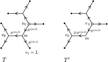
Figure 2: . Illustration of the proof of Lemma 4.9. The tree $T^{\prime}$ is obtained by taking the leaf $v_{1}=L$ off the tree $T$.

By successive applications of Lemma 4.9 to all leaves in $A\setminus\{\alpha\}\subset L(T)$ (that is, marginalizing over all leaves in $A\setminus\{\alpha\}$) we obtain a map

$$f_{A\setminus\alpha}:\bigotimes_{l\in L(T)}W_{l}\longrightarrow\bigotimes_{l\in L(T_{B})}W_{l}$$

that sends the variety $CV_{G}(T)$ to $CV_{G}(T_{B})$.

In order to induce equations from $T_{A}$, $T_{B}$ to $T$, below we translate this map in terms of the corresponding affine coordinate rings. We do not explicitly write indeterminates nor coordinates because the above map $f_{A\setminus\alpha}$ is basis independent. This fact will play an important role in the proof of the main result in the next section.

The map $f_{A\setminus\{\alpha\}}$ above is dual to the map

$$\bigotimes_{l\in L(T_{B})}W_{l}^{*}\rightarrow\bigotimes_{l\in L(T)}W_{l}^{*}$$

that maps $t$ to $\mathbf{1}^{a-1}\otimes t$ if the leaf $L_{B}$ of $T_{B}$ is identified with the leaf $\alpha$ of $T$, so $f_{A\setminus\{\alpha\}}^{*}$ is the map corresponding to $f_{A\setminus\{\alpha\}}$ in terms of coordinates. Moreover, both maps restrict to $G$-invariant vectors. Summing up we have:

Corollary 4.10

Any equation vanishing on $CV_{G}(T_{B})$ extends to an equation vanishing on $CV_{G}(T)$ via the map:

$$\begin{array}[]{ccc}f^{*}_{A\setminus\alpha}:\left(\bigotimes_{l\in L(T_{B})}W_{l}^{*}\right)^{G}&\longrightarrow&\left(\bigotimes_{l\in L(T)}W_{l}^{*}\right)^{G}\\ t&\mapsto&\mathbf{1}^{a-1}\otimes t\end{array}$$

where the leaf $L_{B}$ of $T_{B}$ is identified with the leaf $\alpha$ of $T$.

Similarly, for any subsets $R\subsetneq S\subset L(T)$ of leaves of $T$ we have $f_{S}^{*}$ is the map

$$\begin{array}[]{rcl}f_{S}^{*}:\bigotimes_{l\in R\setminus S}W_{l}^{*}&\longrightarrow&\bigotimes_{l\in R}W_{l}^{*}\\ \otimes_{l\in R\setminus S}v_{l}&\mapsto&\otimes_{l\in R}w_{l}\,,\end{array}$$

where $w_{l}=v_{l}$ if $l\in R\setminus S$ and $w_{l}=\mathbf{1}$ if $l\in S$.

Remark 4.11

It is convenient to write the equations of $T_{B}$ in the basis related to a bipartition $L_{B}|B$. In this way, the extension of a coordinate as defined in Corollary 4.10 gives rise to a coordinate that is already in the basis $\mathcal{B}_{A|B}$ of $(\otimes W^{n})^{G}$ (indeed, as $\mathbf{1}$ is $G$-invariant, the operator (4.1) does not affect it and it is easy to check that the extended basis are elements of $\mathcal{B}_{A|B}$).

5 The main result

Given a phylogenetic tree under an equivariant model $\mathcal{M}_{G}$, the goal of this section is to construct a complete intersection for $CV_{G}(T)$ on a neighborhood of a point of no evolution. This will be done by using induction on the number of leaves of the tree.

Let $T$ be a tree with at least one interior edge and leaves $L(T)=\{l_{1},\ldots,l_{n}\}$. Reordering the set of leaves (if needed) we can assume that there exists a node with children $\{l_{n-l},\dots,l_{n}\}$, $l\geq 1$. We take the edge split $A|B$ given by $A=\{l_{1},\ldots,l_{n-l-1}\}$, $B=\{l_{n-l},\dots,l_{n}\}$. Write $e$ for the interior edge of $T$ associated with this split. Keeping the notation already used throughout the paper, $T_{A}$ has leaves $A\cup\{L_{A}\}$, $T_{B}$ has leaves $B\cup\{L_{B}\}$ (where $L_{A}$, $L_{B}$ are defined as in figure 1). The variety associated to $T_{A}$ is the closure of the image of the polynomial map

$$\Psi_{T_{A}}:\mathrm{Par}_{G}(T_{A})\rightarrow\otimes^{n-l}W^{G}.$$

and the variety $CV_{G}(T_{B})\subset\otimes^{l+2}W^{G}$ is the closure of the image of

$$\Psi_{T_{B}}:\mathrm{Par}_{G}(T_{B})\rightarrow\otimes^{l+2}W^{G}.$$

Lemma 5.1

Given a leaf $L$ in $T$, the image of a point of no evolution $\pi_{n}\in\otimes^{n}W$ under the map $f_{L}$ is a point of no evolution in $\otimes^{n-1}W$.

Proof. If $\pi_{n}=\sum_{\mathtt{X}\in\Sigma}\pi_{\mathtt{X}}\mathtt{X}\otimes\ldots\otimes\mathtt{X}$, then its image under the map $f_{L}$ is

$$f_{L}(\pi_{n})=\sum_{\mathtt{X}\in\Sigma}\pi_{\mathtt{X}}(\mathbf{1}\cdot\mathtt{X})^{a}\left(\mathtt{X}\otimes\stackrel{{\scriptstyle n-a}}{{\ldots}}\otimes\mathtt{X}\right)=\sum_{\mathtt{X}\in\Sigma}\pi_{\mathtt{X}}\mathtt{X}\otimes\stackrel{{\scriptstyle n-a}}{{\ldots}}\otimes\mathtt{X}.$$

As $\pi_{n}$ was invariant by the action of $G$, so is $f_{L}(\pi_{n})$ and therefore it is a point of no evolution in $\otimes^{n-a}W$. $\square$

By successively applying the above lemma and lemma 4.9 we obtain points of no evolution in $CV_{G}(T_{A})$ and in $CV_{G}(T_{B})$ from a point of no evolution $\pi_{n}$ in $CV_{G}(T)$. This shall allow us to apply an induction argument.

Let $T_{d}$ be the claw tree with $d$ leaves (claw $d$-tree) evolving under $\mathcal{M}_{G}$ and $L(T_{d})=\{x_{0},\dots,x_{d-1}\}$, and let $\mathfrak{eq}_{T_{d}}:=\{h_{1},h_{2},\ldots,h_{\mathrm{codim}\,(CV_{G}(T_{d}))}\}$ be a set of equations of a complete intersection that defines $CV_{G}(T_{d})\subset(\otimes^{d}W)^{G}$ on an open subset containing general points of no evolution. As we already proved, general points of no evolution are smooth by Theorem 3.8. In particular, the variety is locally a complete intersection, which guaranties the existence of $\mathfrak{eq}_{T_{d}}$. Before proceeding with induction, we need the following assumption about the equivariant model $\mathcal{M}_{G}$ on the claw tree with $d$ leaves, which shall be checked for every particular equivariant model and every $d$ equal to a degree of one of the interior nodes of $T$. For the GMM, the strand symmetric model, and the Jukes-Cantor model, we prove in section 6 that this assumption holds for the tripod (and hence our result is valid for trivalent trees evolving on these models). A local complete intersection for the Kimura 3-parameter model for trivalent trees was already given in [13].

Claw $d$-tree hypothesis 5.2

We write equations $\mathfrak{eq}_{T_{d}}$ on a basis of type $\mathcal{B}_{x_{0}\mid\{x_{1},\dots,x_{d-1}\}}$ following subsection 4.2. The jacobian of these new equations $\mathfrak{eq}_{B}$ , which we denote as $\mathbf{J}_{x_{0}\mid x_{1},\cdot,x_{d-1}}(T_{d})$, has rank equal to $\mathrm{codim}\,(CV_{G}(T_{d}))$ at any general point of no evolution. We denote by $\mathbf{J}_{x_{0}\mid x_{1},\cdot,x_{d-1}}^{*}(T_{d})$ the matrix obtained from $\mathbf{J}_{x_{0}\mid x_{1},\cdot,x_{d-1}}(T_{d})$ by removing the columns corresponding to $S(u^{k}_{x_{0},i}\otimes u^{k}_{x_{1},\cdot,x_{d-1},j})$ for $k=1\div t$ and $i,j=1\div m_{k}$. We say that the equivariant model $\mathcal{M}_{G}$ satisfies the claw $d$-tree hypothesis if

$$\mathrm{rank}\,\,\mathbf{J}_{x_{0}\mid x_{1},\cdot,x_{l-d}}^{*}(T_{d})=\mathrm{codim}\,(CV_{G}(T_{d})),$$ (8)

whenever this matrix is evaluated at a generic point of no evolution.

Induction hypothesis.

We will use the following induction hypothesis:

$(\ast)$ There is a set of equations $\mathfrak{eq}_{T_{A}}=\{g_{1},g_{2},\ldots,g_{\mathrm{codim}\,(CV_{G}(T_{A}))}\}$ that defines the variety $CV_{G}(T_{A})\subset(\otimes^{n-l}W)^{G}$ scheme theoretically on an open subset containing general points of no evolution.

By Corollary 4.10, the map $\tau\mapsto\tau\otimes\mathbf{1}^{l}$ induces new equations for $CV_{G}(T)$ from $\mathfrak{eq}_{T_{A}}$. These equations shall be written in the coordinates $q^{k}_{i,j}$ corresponding to the basis $\mathcal{B}_{A|B}$ linked to the edge split $A|B$ and shall be called $\mathfrak{eq}_{A}=\{f^{A}_{1},\ldots,f^{A}_{\mathrm{codim}\,(CV_{G}(T_{A}))}\}\subset\mathbb{C}[q^{k}_{i,j}]$.

As above, by Corollary 4.10, the map $\tau\mapsto\mathbf{1}^{n-l-2}\otimes\tau$ induces new equations

$$\mathfrak{eq}_{B}=\{f^{B}_{1},\ldots,f^{B}_{\mathrm{codim}\,(CV_{G}(T_{B})}\}\subset\mathbb{C}[q^{k}_{i,j}]$$

for $CV_{G}(T)$ from the set of equations $\mathfrak{eq}_{T_{B}}$ of the underlying model assumption.

Besides, we still need to consider the set of polynomials coming from the edge split.

Edge invariants.

As in subsection 4.2, for each $k=1,\ldots,t$, write $M_{k}$ for the ${m_{k}(n-l-1)}\times{m_{k}(l+1)}$-matrix with rows indexed by the $u^{k^{*}}_{A,i}$, $i=1,\ldots,m_{k}(n-l-1)$, columns indexed by $u^{k}_{B,j}$, $j=1,\ldots,m_{k}(l+1)$, and whose $(i,j)$-entry is the coordinate $q^{k}_{i,j}$. For each of these matrices, take the set of all the $(m_{k}+1)\times(m_{k}+1)$-minors containing the sub matrix $M_{k}^{0}$ defined in Section 4.2, with rows and columns indexed by $\{u^{k^{*}}_{A,i}\}_{i=1,\ldots,m_{k}}$ and $\{u^{k}_{B,j}\}_{j=1,\ldots,m_{k}}$, respectively. We obtain $N_{A|B}$ polynomials in $\mathbb{C}[q^{k}_{i,j}]$ of the form (6).

Lemma 5.3

We have $\mathrm{codim}\,(CV_{G}(T_{A}))+\mathrm{codim}\,(CV_{G}(T_{B})+N_{A|B}=\mathrm{codim}\,(CV_{G}(T))$.

Proof.

We assume that $T$ has no vertices of degree $2$, as such nodes can be removed. By Theorem 3.5 and Remark 4.7, we have

$$\mathrm{codim}\,(CV_{G}(T_{A}))+\mathrm{codim}\,(CV_{G}(T_{B})+N_{A|B}=$$

$$\left(m_{1}(l+2)-(|E(T)|-(n-l-1))(m_{1}(2)-m_{1})-m_{1}\right)+$$

$$\left(m_{1}(n)-m_{1}(n-l)-m_{1}(l+2)+m_{1}(2)\right)+$$

$$+\left(m_{1}(n-l)-(n-l)(m_{1}(2)-m_{1})-m_{1}\right).$$

The sum above equals

$$m_{1}(n)-|E(T)|(m_{1}(2)-m_{1})-m_{1}=\mathrm{codim}\,(CV_{G}(T)).$$

$\square$

Theorem 5.4

Let $T$ be a phylogenetic tree on $n$ leaves, $n\geq 3$; let $D$ be the set of degrees of its interior nodes, and assume that $d\geq 3$ for any $d\in D$. Let $\mathcal{M}_{G}$ be an equivariant model that satisfies the claw $d$-tree hypothesis for any $d\in D$. The set of equations $\mathfrak{eq}_{T}:=\mathfrak{eq}_{A}\cup\mathfrak{eq}_{B}\cup\mathfrak{eq}_{A|B}$ defines the variety $CV_{G}(T)$ scheme theoretically on an open subset that contains general points of no evolution.

Proof. We proceed by induction on the number of leaves. The first step is $n=3$, which is covered by the claw $d$-tree assumption for $d=3$. We assume thus $n>3$ and that $T$ has at least one interior edge which splits the leaves $L(T)=\{l_{1},\ldots,l_{n}\}$ into two sets $A=\{l_{1},\ldots,l_{n-l-1}\}$ and $B=\{l_{n-l},\dots,l_{n}\}$ (reordering leaves if necessary). Consider the trees $T_{A}$ and $T_{B}$ as defined in the beginning of this section. Note that we are able to use the induction hypothesis stated above because the set of degrees for the interior nodes of the tree $T_{A}$ is included in $D$. By Lemma 5.3, we know that

$$|\mathfrak{eq}_{A}|+|\mathfrak{eq}_{B}|+|\mathfrak{eq}_{A|B}|=\mathrm{codim}\,(CV_{G}(T)),$$

that is, the number of equations equals the codimension of the variety. We already know that $\mathfrak{eq}_{T}$ are equations satisfied by all points in $CV_{G}(T)$.

Let $V^{\prime}$ be the variety defined by $\mathfrak{eq}_{T}$. Now, consider the jacobian matrix $\mathbf{J}_{A|B}(T)$ obtained by taking the partial derivatives of the polynomials in $\mathfrak{eq}_{A|B}$ with respect to the coordinates $q^{k}_{i,j}$ of $(\otimes^{n}W)^{G}$. We claim that the rank of this matrix at a generic point of no evolution $\pi_{n}$ is maximal. From this, we will deduce that $V^{\prime}$ is non-singular in a neighborhood $U$ of $\pi_{n}$. Since $V^{\prime}$ and $CV_{G}(T)$ have the same dimension, it follows that both varieties are equal in $U$.

By reordering the columns of the jacobian matrix if necessary, we may assume that columns are indexed as follows:

• the first $m_{1}(n-l)-m_{1}(2)$ columns are indexed by $q^{k}_{i,j}$ with ${i=m_{k}+1\div m_{k}(n-l-1)}$, ${j=1\div m_{k}}$, ${k=1\div t}$;

• then, $m_{1}(2)$ columns indexed by $q^{k}_{i,j}$ with $i=1\div m_{k}$, $j=1\div m_{k}$, $k=1\div t$;

• then, $m_{1}(l+2)-m_{1}(2)$ columns indexed by $q^{k}_{i,j}$ with $i=1\div m_{k}$, $j=m_{k}+1\div m_{k}(l+1)$, $k=1\div t$;

• the remaining columns correspond to $i=m_{k}+1\div m_{k}(n-l-1)$, $j=m_{k}+1\div m_{k}(l+1)$, $k=1\div t$.

Notice that the equations in $\mathfrak{eq}_{A}$ only have coordinates in the first $m_{1}(n-l)$ columns and $\mathfrak{eq}_{B}$ only in the middle $m_{1}(l+2)$ columns. With this ordering, the jacobian matrix has the form

$$\mathbf{J}_{A|B}(T)=\left(\;\begin{array}[]{ccccccc}\cline{1-4}\cr\vrule\lx@intercol\hfil\mathbf{J}_{A|L_{A}}(T_{A})\hfil\lx@intercol\vrule\lx@intercol&0&\lx@intercol\hfil\quad 0\hfil\lx@intercol\\ \cline{1-5}\cr\lx@intercol\hfil\quad*\hfil\lx@intercol&\vrule\lx@intercol\hfil\mathbf{J}_{L_{B}|B}(T_{B})\hfil\lx@intercol\vrule\lx@intercol&\lx@intercol\hfil\quad 0\hfil\lx@intercol\\ \cline{1-7}\cr\vrule\lx@intercol\hfil\frac{\partial}{\partial\,q^{k}_{i,j}}E^{k}_{i,j}\hfil\lx@intercol\vrule\lx@intercol\\ \cline{1-7}\cr\end{array}\;\right)$$

where:

1. The first block $\mathbf{J}_{A|L_{A}}(T_{A})$ has $\mathrm{codim}\,(CV_{T_{A}})$ rows, and $m_{1}(n-l)$ columns indexed by the coordinates in $(\otimes^{n-l}W)^{G}$ extended to $(\otimes^{n}W)^{G}$.

2. The second block $\mathbf{J}_{L_{B}|B}(T_{B})$ has $\mathrm{codim}\,(CV_{T_{B}})$ rows, and $m_{1}(l+2)$ columns indexed by the coordinates in $(\otimes^{l+2}W)^{G}$ extended to $(\otimes^{n}W)^{G}$.

Notice that the first two blocks share the columns indexed by the coordinates $\{q^{k}_{i,j}\}_{1\leq i,j\leq m_{k}}$.

1. The third block $\big{(}\frac{\partial}{\partial\,q^{k}_{i,j}}E^{k}_{i,j}\big{)}$ has $N_{n-l-1|l+1}$ rows, indexed by the equations of $\mathfrak{eq}^{n}_{A|B}$, and $m_{1}(n)$ columns, indexed by all the coordinates above: $\{q^{k}_{i,j}\}_{1\leq i\leq m_{k}(l+1),1\leq j\leq m_{k}(n-l-1),1\leq k\leq t}$.

From now on, these coordinates refer to a generic point of no evolution $\pi_{n}.$

We proceed by induction on the number of leaves and the induction hypothesis applied is the one explained above the statement of the theorem. By the induction hypothesis we know that the rank of $\mathbf{J}_{A\mid L_{A}}(T_{A})$ is equal to $\mathrm{codim}\,(CV_{T_{A}})$. By the claw $d$-tree hypothesis (8), we know that

$$\mathbf{J}_{L_{B}|B}(T_{B})=\left[\begin{array}[]{cc|r}*&*&\\ &*&\mathbf{J}_{L_{B}|B}^{*}(T_{B})\\ &*&\end{array}\right]$$

and the rank of $\mathbf{J}_{L_{B}|B}^{*}(T_{B})$ is equal to $\mathrm{codim}\,(CV_{T_{B}})$. This assures that the first $\mathrm{codim}\,(CV_{T_{B}})+\mathrm{codim}\,(CV_{T_{A}})$ rows in the matrix are linearly independent. For the third block and by virtue of Lemma 4.8, we have

$$\Big{[}\frac{\partial}{\partial\,q^{k}_{i,j}}E^{k}_{i,j}\Big{]}=\left[\begin{array}[]{cccc}*&\ldots&\ldots&*\\ &&&*\\ &\ldots&\ldots&*\end{array}\right|\left.\begin{array}[]{c}\\ \operatorname{Diag}(\Delta_{k}(\pi_{n}))\\ \end{array}\right]$$

where $\operatorname{Diag}(\Delta_{k}(\pi_{n}))$ is the diagonal matrix with entries $\{\Delta_{k}(\pi_{n})\}_{k}$ and columns indexed by the coordinates $q^{k}_{i,j}$ for $i,j\geq m_{k}+1$. By Lemma 5.5 below, these entries are nonzero. We conclude that the rank of $\mathbf{J}_{A|B}(T)$ is maximal and equal to $\mathrm{codim}\,(CV_{T})$. $\square$

Lemma 5.5

Let $\pi_{n}$ be a generic point of no evolution. Then, $\Delta_{k}(\pi_{n})\neq 0$ for every $k=1,\ldots,t$.

Proof. The matrix $M^{0}_{k}$ for any tensor in $p\in(\otimes^{n}W)^{G}$ represents a tensor in $\mathcal{F}_{k^{*}}(W_{\alpha})\otimes\mathcal{F}_{k}(W_{\beta})$ obtained as follows:

1. first contract $p$ with $f_{L(T)\setminus\{\alpha,\beta\}}$ to obtain a tensor $p^{\prime}$ in $(W_{\alpha}\otimes W_{\beta})^{G}$,

2. project $p^{\prime}$ according to the decomposition $(W_{\alpha}\otimes W_{\beta})^{G}\cong\bigoplus_{k}\mathcal{F}_{k^{*}}(W_{\alpha})\otimes\mathcal{F}_{k}(W_{\beta})$.

The determinant of $M_{k}^{0}$ is nonzero if and only if the associated map $\mathcal{F}_{k}(W_{\alpha}^{*})\rightarrow\mathcal{F}_{k}(W_{\beta})$ has maximal rank, i.e. is an isomorphism. However, this is the case for all $k$ if and only if $p^{\prime}$ defines a $G$-isomorphism $W_{\alpha}^{*}\rightarrow W_{\beta}$.

By lemma 5.1, the marginalization of $\pi_{n}=\sum_{\mathtt{X}\in\Sigma}\pi_{\mathtt{X}}\mathtt{X}\otimes\ldots\otimes\mathtt{X}$ over all leaves different from $\alpha$ and $\beta$ provides a tensor $p^{\prime}=\sum_{{\mathtt{X}}\in\Sigma}\pi_{\mathtt{X}}{\mathtt{X}}\otimes{\mathtt{X}}$. This tensor corresponds to the map from $W_{\alpha}^{*}$ to $W_{\beta}$ whose matrix in basis $\{X_{i}\}$ is diagonal with entries $\pi_{X_{i}}$. Therefore, if the coordinates $\pi_{X}$ of $\pi_{n}$ are all non-zero, this is an isomorphism and therefore the matrices $M^{0}_{k}$ have non-zero determinant for all $k$. This proves the claim. $\square$

Remark 5.6

The list of equations for a phylogenetic tree as in Theorem 5.4 is obtained from edge invariants and from local equations for $d$-claw trees, $d\in D$. As pointed out in 4.7, the number of edge invariants is exponential in $n$ (at least for the usual models) and can be substituted by a direct evaluation of the rank of the thin flattening. It is worth noticing that the other subset of equations, the ones coming from $d$-claw trees, are at most exponential in $d$ and therefore this subset can reasonably be used in practice.

6 Explicit equations for usual models

The aim of this section is to provide explicit examples of complete intersections of the particular models listed in Example 3.4. For the Kimura 3-parameter, this was already done in [13]; here we deal with GMM, strand symmetric and Jukes-Cantor models (the only remaining case would be Kimura 2-parameter, for which the tripod assumption could be checked using computational algebra software).

As mentioned in Example 4.3, for these models we can use the Fourier basis to span the isotypic components of $W$. In this cases, we can identify $\underline{\Sigma}$ with the group $(\mathbb{Z}_{2}\times\mathbb{Z}_{2},+)$ via

$$\underline{\mathtt{A}}\mapsto(0,0);\quad\underline{\mathtt{C}}\mapsto(1,0);\quad\underline{\mathtt{G}}\mapsto(0,1);\quad\underline{\mathtt{T}}\mapsto(1,1).$$ (12)

We denote by $\chi_{\mathtt{A}}$, $\chi_{\mathtt{C}}$, $\chi_{\mathtt{G}}$, $\chi_{\mathtt{T}}$ the characters associated to this group $(\mathbb{Z}_{2}\times\mathbb{Z}_{2},+)$ (see table 2). These characters are useful to describe the coordinates of a point of no evolution.

	$\underline{\mathtt{A}}$	$\underline{\mathtt{C}}$	$\underline{\mathtt{G}}$	$\underline{\mathtt{T}}$
$\chi_{\mathtt{A}}$	1	1	1	1
$\chi_{\mathtt{C}}$	1	1	-1	-1
$\chi_{\mathtt{G}}$	1	-1	1	-1
$\chi_{\mathtt{T}}$	1	-1	-1	1

Table 2: Description of characters $\chi_{\mathtt{A}}$, $\chi_{\mathtt{C}}$, $\chi_{\mathtt{G}}$, $\chi_{\mathtt{T}}$ for the group $(\mathbb{Z}_{2}\times\mathbb{Z}_{2},+)$.

Lemma 6.1

If $\pi_{n}$ is a point of no evolution, then $\pi_{n}=\sum_{\underline{\mathtt{Y}}_{1},\ldots,\underline{\mathtt{Y}}_{n}}q_{\underline{\mathtt{Y}}_{1},\ldots,\underline{\mathtt{Y}}_{n}}\underline{\mathtt{Y}}_{1}\ldots\underline{\mathtt{Y}}_{n}$, where

$$q_{\underline{\mathtt{Y}}_{1},\ldots,\underline{\mathtt{Y}}_{n}}=\frac{1}{4^{n}}\left(\pi_{\mathtt{A}}+\chi_{\mathtt{C}}(\underline{\mathtt{Y}})\pi_{\mathtt{C}}+\chi_{\mathtt{G}}(\underline{\mathtt{Y}})\pi_{\mathtt{G}}+\chi_{\mathtt{T}}(\underline{\mathtt{Y}})\pi_{\mathtt{T}}\right),$$

$\underline{\mathtt{Y}}:=\underline{\mathtt{Y}}_{1}+\ldots+\underline{\mathtt{Y}}_{n}$ with the operation given by the identification (12).

Proof. From the definition of the Fourier basis in 4.1.1 and using Table 2, we have $\mathtt{X}=\frac{1}{4}\sum_{\underline{\mathtt{Y}}\in\underline{\Sigma}}\chi_{\mathtt{X}}(\underline{\mathtt{Y}})\,\underline{\mathtt{Y}}$, for any $\mathtt{X}\in\Sigma$. Now, using that characters of 1-dimensional representations are multiplicative, if $\pi_{n}$ is a point of no evolution we have

$$\pi_{n} = \sum_{\mathtt{X}}\pi_{\mathtt{X}}\mathtt{X}\otimes\ldots\otimes\mathtt{X}=$$

$$= \sum_{\mathtt{X}}\;\frac{\pi_{\mathtt{X}}}{4^{n}}\;\Big{(}\sum_{\underline{\mathtt{Y}}_{1}}\chi_{\mathtt{X}}(\underline{\mathtt{Y}}_{1})\,\underline{\mathtt{Y}}_{1}\Big{)}\otimes\ldots\otimes\Big{(}\sum_{\underline{\mathtt{Y}}_{n}}\chi_{\mathtt{X}}(\underline{\mathtt{Y}}_{n})\,\underline{\mathtt{Y}}_{n}\Big{)}=$$

$$= \sum_{\mathtt{X}}\;\frac{\pi_{\mathtt{X}}}{4^{n}}\;\sum_{\underline{\mathtt{Y}}_{1},\underline{\mathtt{Y}}_{2},\ldots,\underline{\mathtt{Y}}_{n}}\chi_{\mathtt{X}}(\underline{\mathtt{Y}}_{1})\chi_{\mathtt{X}}(\underline{\mathtt{Y}}_{2})\ldots\chi_{\mathtt{X}}(\underline{\mathtt{Y}}_{n})\;\underline{\mathtt{Y}}_{1}\,\underline{\mathtt{Y}}_{2}\,\ldots\,\underline{\mathtt{Y}}_{n}=$$

$$= \sum_{\mathtt{X}}\;\frac{\pi_{\mathtt{X}}}{4^{n}}\;\sum_{\underline{\mathtt{Y}}_{1},\underline{\mathtt{Y}}_{2},\ldots,\underline{\mathtt{Y}}_{n}}\chi_{\mathtt{X}}(\underline{\mathtt{Y}}_{1}+\underline{\mathtt{Y}}_{2}+\ldots+\underline{\mathtt{Y}}_{n})\;\underline{\mathtt{Y}}_{1}\,\underline{\mathtt{Y}}_{2}\,\ldots\,\underline{\mathtt{Y}}_{n}=$$

$$= \sum_{\underline{\mathtt{Y}}_{1},\underline{\mathtt{Y}}_{2},\ldots,\underline{\mathtt{Y}}_{n}}\left(\frac{1}{4^{n}}\sum_{\mathtt{X}}\;\pi_{\mathtt{X}}\;\chi_{\mathtt{X}}(\underline{\mathtt{Y}})\right)\;\underline{\mathtt{Y}}_{1}\,\underline{\mathtt{Y}}_{2}\,\ldots\,\underline{\mathtt{Y}}_{n}.$$

From this, the claim follows. $\square$

Figure 3: .

6.1 Equations for trees evolving under the Jukes-Cantor model

Take the Jukes-Cantor model, this is, $G=\mathfrak{S}_{4}$. There are five irreducible representations of the group $G$: $N_{1},\dots,N_{5}$ (see [31] $\S$2.3). For each $i=1\div 5$, the representation $N_{i}$ has the character $\chi_{i}$ shown in Table 1. As in Example 4.3.5, we have $u^{1}_{1}=\underline{\mathtt{A}}$, $u^{4}_{1}=\underline{\mathtt{C}}$ and $\mathcal{F}_{1}(W)=\langle\underline{\mathtt{A}}\rangle$ and $\mathcal{F}_{4}(W)=\langle\underline{\mathtt{C}}\rangle$. By letting the group $G$ act, it follows that $W=W[\chi_{1}]\oplus W[\chi_{4}]$, with $W[\chi_{1}]=\langle\underline{\mathtt{A}}\rangle$ and $W[\chi_{4}]=\langle\underline{\mathtt{C}},\underline{\mathtt{G}},\underline{\mathtt{T}}\rangle$.

We take the tree $T$ with 4 leaves $12|34$ and take the bipartition $A=\{1,2\}$ and $B=\{3,4\}$. We proceed to obtain a basis for the ambient space $(\otimes^{4}W)^{G}$ of the variety $V_{T}$. Choose $\alpha=2$ and $\beta=3$ as in figure 3. Following the algorithm described, and noting that $\chi^{2}=2\chi_{1}+\chi_{3}+3\chi_{4}+\chi_{5}$, we obtain the following basis

Now, for each of the irreducible representations of $\mathfrak{S}_{4}$, we can choose a subgroup $H_{k}$ so that $\{hu^{k}_{A,i}\mid h\in H_{k}\}$ is a basis of the representation spanned by the $\mathfrak{S}_{4}$-orbit of $u^{k}_{A,i}$. Namely,

$$H_{1}=\{e\} n_{1}=1;$$

$$H_{3}=\{e,(\mathtt{A}\mathtt{C})\} n_{3}=2;$$

$$H_{4}=\{e,(\mathtt{C}\mathtt{G}\mathtt{T}),(\mathtt{C}\mathtt{T}\mathtt{G})\} n_{4}=3;$$

$$H_{5}=\{e,(\mathtt{C}\mathtt{G}\mathtt{T}),(\mathtt{C}\mathtt{T}\mathtt{G})\} n_{5}=3.$$

A basis for $(W_{A}\otimes W_{B})^{G}$ is inferred from $\bigoplus_{k}\mathcal{F}_{k}(W_{A})\otimes\mathcal{F}_{k}(W_{B})$ by taking the image of the operator $S$ specified in Remark 4.1 applied to the tensors $u^{k}_{A,i}\otimes u^{k}_{B,j}$:

$$S(u^{k}_{A,i}\otimes u^{k}_{B,j}):=\frac{n_{k}}{|G|}\sum_{g\in G}(g\cdot u^{k}_{A,i})\otimes(g\cdot u^{k}_{B_{j}}),$$

that is,

$$S(u^{1}_{A,1}\otimes u^{1}_{B,1}) = \underline{\mathtt{A}}\underline{\mathtt{A}}\underline{\mathtt{A}}\underline{\mathtt{A}},$$

$$S(u^{1}_{A,1}\otimes u^{1}_{B,2}) = \frac{1}{3}\underline{\mathtt{A}}\underline{\mathtt{A}}\otimes(\underline{\mathtt{C}}\underline{\mathtt{C}}+\underline{\mathtt{G}}\underline{\mathtt{G}}+\underline{\mathtt{T}}\underline{\mathtt{T}}),$$

$$S(u^{1}_{A,2}\otimes u^{1}_{B,1}) = \frac{1}{3}(\underline{\mathtt{C}}\underline{\mathtt{C}}+\underline{\mathtt{G}}\underline{\mathtt{G}}+\underline{\mathtt{T}}\underline{\mathtt{T}})\otimes\underline{\mathtt{A}}\underline{\mathtt{A}},$$

$$S(u^{1}_{A,2}\otimes u^{1}_{B,2}) = \frac{1}{3}(\underline{\mathtt{C}}\underline{\mathtt{C}}+\underline{\mathtt{G}}\underline{\mathtt{G}}+\underline{\mathtt{T}}\underline{\mathtt{T}})\otimes(\underline{\mathtt{C}}\underline{\mathtt{C}}+\underline{\mathtt{G}}\underline{\mathtt{G}}+\underline{\mathtt{T}}\underline{\mathtt{T}}),$$

$$S(u^{3}_{A,1}\otimes u^{3}_{B,1}) = \frac{2}{3}\big{(}(\underline{\mathtt{C}}\underline{\mathtt{C}}-\underline{\mathtt{G}}\underline{\mathtt{G}})\otimes(\underline{\mathtt{C}}\underline{\mathtt{C}}-\underline{\mathtt{G}}\underline{\mathtt{G}})+(\underline{\mathtt{G}}\underline{\mathtt{G}}-\underline{\mathtt{T}}\underline{\mathtt{T}})\otimes(\underline{\mathtt{G}}\underline{\mathtt{G}}-\underline{\mathtt{T}}\underline{\mathtt{T}})+(\underline{\mathtt{T}}\underline{\mathtt{T}}-\underline{\mathtt{C}}\underline{\mathtt{C}})\otimes(\underline{\mathtt{T}}\underline{\mathtt{T}}-\underline{\mathtt{C}}\underline{\mathtt{C}})\big{)}$$

$$S(u^{4}_{A,1}\otimes u^{4}_{B,1}) = \underline{\mathtt{A}}\underline{\mathtt{C}}\underline{\mathtt{C}}\underline{\mathtt{A}}+\underline{\mathtt{A}}\underline{\mathtt{G}}\underline{\mathtt{G}}\underline{\mathtt{A}}+\underline{\mathtt{A}}\underline{\mathtt{T}}\underline{\mathtt{T}}\underline{\mathtt{A}},$$

$$S(u^{4}_{A,1}\otimes u^{4}_{B,2}) = \underline{\mathtt{A}}\underline{\mathtt{C}}\underline{\mathtt{A}}\underline{\mathtt{C}}+\underline{\mathtt{A}}\underline{\mathtt{G}}\underline{\mathtt{A}}\underline{\mathtt{G}}+\underline{\mathtt{A}}\underline{\mathtt{T}}\underline{\mathtt{A}}\underline{\mathtt{T}},$$

$$S(u^{4}_{A,1}\otimes u^{4}_{B,3}) = \underline{\mathtt{A}}\underline{\mathtt{C}}\otimes(\underline{\mathtt{G}}\underline{\mathtt{T}}+\underline{\mathtt{T}}\underline{\mathtt{G}})+\underline{\mathtt{A}}\underline{\mathtt{G}}\otimes(\underline{\mathtt{C}}\underline{\mathtt{T}}+\underline{\mathtt{T}}\underline{\mathtt{C}})+\underline{\mathtt{A}}\underline{\mathtt{T}}\otimes(\underline{\mathtt{C}}\underline{\mathtt{G}}+\underline{\mathtt{G}}\underline{\mathtt{C}}),$$

$$S(u^{4}_{A,2}\otimes u^{4}_{B,1}) = \underline{\mathtt{C}}\underline{\mathtt{A}}\underline{\mathtt{C}}\underline{\mathtt{A}}+\underline{\mathtt{G}}\underline{\mathtt{A}}\underline{\mathtt{G}}\underline{\mathtt{A}}+\underline{\mathtt{T}}\underline{\mathtt{A}}\underline{\mathtt{T}}\underline{\mathtt{A}},$$

$$S(u^{4}_{A,2}\otimes u^{4}_{B,2}) = \underline{\mathtt{C}}\underline{\mathtt{A}}\underline{\mathtt{A}}\underline{\mathtt{C}}+\underline{\mathtt{G}}\underline{\mathtt{A}}\underline{\mathtt{A}}\underline{\mathtt{G}}+\underline{\mathtt{T}}\underline{\mathtt{A}}\underline{\mathtt{A}}\underline{\mathtt{T}},$$

$$S(u^{4}_{A,2}\otimes u^{4}_{B,3}) = \underline{\mathtt{C}}\underline{\mathtt{A}}\otimes(\underline{\mathtt{G}}\underline{\mathtt{T}}+\underline{\mathtt{T}}\underline{\mathtt{G}})+\underline{\mathtt{G}}\underline{\mathtt{A}}\otimes(\underline{\mathtt{C}}\underline{\mathtt{T}}+\underline{\mathtt{T}}\underline{\mathtt{C}})+\underline{\mathtt{T}}\underline{\mathtt{A}}\otimes(\underline{\mathtt{C}}\underline{\mathtt{G}}+\underline{\mathtt{G}}\underline{\mathtt{C}}),$$

$$S(u^{4}_{A,4}\otimes u^{4}_{B,1}) = (\underline{\mathtt{G}}\underline{\mathtt{T}}+\underline{\mathtt{T}}\underline{\mathtt{G}})\otimes\underline{\mathtt{C}}\underline{\mathtt{A}}+(\underline{\mathtt{C}}\underline{\mathtt{T}}+\underline{\mathtt{T}}\underline{\mathtt{C}})\otimes\underline{\mathtt{G}}\underline{\mathtt{A}}+(\underline{\mathtt{C}}\underline{\mathtt{G}}+\underline{\mathtt{G}}\underline{\mathtt{C}})\otimes\underline{\mathtt{T}}\underline{\mathtt{A}},$$

$$S(u^{4}_{A,3}\otimes u^{4}_{B,2}) = (\underline{\mathtt{G}}\underline{\mathtt{T}}+\underline{\mathtt{T}}\underline{\mathtt{G}})\otimes\underline{\mathtt{A}}\underline{\mathtt{C}}+(\underline{\mathtt{C}}\underline{\mathtt{T}}+\underline{\mathtt{T}}\underline{\mathtt{C}})\otimes\underline{\mathtt{A}}\underline{\mathtt{G}}+(\underline{\mathtt{C}}\underline{\mathtt{G}}+\underline{\mathtt{G}}\underline{\mathtt{C}})\otimes\underline{\mathtt{A}}\underline{\mathtt{T}},$$

$$S(u^{4}_{A,3}\otimes u^{4}_{B,3}) = (\underline{\mathtt{G}}\underline{\mathtt{T}}+\underline{\mathtt{T}}\underline{\mathtt{G}})\otimes(\underline{\mathtt{G}}\underline{\mathtt{T}}+\underline{\mathtt{T}}\underline{\mathtt{G}})+(\underline{\mathtt{C}}\underline{\mathtt{T}}+\underline{\mathtt{T}}\underline{\mathtt{C}})\otimes(\underline{\mathtt{C}}\underline{\mathtt{T}}+\underline{\mathtt{T}}\underline{\mathtt{C}})+(\underline{\mathtt{C}}\underline{\mathtt{G}}+\underline{\mathtt{G}}\underline{\mathtt{C}})\otimes(\underline{\mathtt{C}}\underline{\mathtt{G}}+\underline{\mathtt{G}}\underline{\mathtt{C}}),$$

$$S(u^{5}_{A,1}\otimes u^{5}_{B,1}) = (\underline{\mathtt{G}}\underline{\mathtt{T}}-\underline{\mathtt{T}}\underline{\mathtt{G}})\otimes(\underline{\mathtt{G}}\underline{\mathtt{T}}-\underline{\mathtt{T}}\underline{\mathtt{G}})+(\underline{\mathtt{C}}\underline{\mathtt{T}}-\underline{\mathtt{T}}\underline{\mathtt{C}})\otimes(\underline{\mathtt{C}}\underline{\mathtt{T}}-\underline{\mathtt{T}}\underline{\mathtt{C}})+(\underline{\mathtt{C}}\underline{\mathtt{G}}-\underline{\mathtt{G}}\underline{\mathtt{C}})\otimes(\underline{\mathtt{C}}\underline{\mathtt{G}}-\underline{\mathtt{G}}\underline{\mathtt{C}}).$$

As above, denote by $q^{k}_{i,j}$ the coordinates corresponding to this basis $S(u^{k}_{A,i}\otimes u^{k}_{B,j})$. We proceed to obtain a complete intersection for the tree $T$ with 4 leaves $12|34$. Take the bipartition $A=\{1,2\}$ and $B=\{3,4\}$.

First of all, we proceed to obtain the edge invariants following the section 4.2. If $\pi_{4}$ is a no evolution point, write $\pi_{4}=\sum_{k,i,j}q^{k}_{ij}\,S(u^{k}_{A,i}\otimes u^{k}_{B,j})$. Each irreducible representation $N_{k}$ of $\mathfrak{S}_{4}$ gives rise to a $m_{k}(2)\times m_{k}(2)$-matrix $M_{k}$:

$$M_{1}=\left(\begin{array}[]{cc}q^{1}_{11}&q^{1}_{12}\\ q^{1}_{21}&q^{1}_{22}\end{array}\right),\qquad M_{3}=\left(\begin{array}[]{c}q^{3}_{11}\end{array}\right),\qquad M_{4}=\left(\begin{array}[]{ccc}q^{4}_{11}&q^{4}_{12}&q^{4}_{13}\\ q^{4}_{21}&q^{4}_{22}&q^{4}_{23}\\ q^{4}_{31}&q^{4}_{32}&q^{4}_{33}\end{array}\right),\qquad M_{5}=\left(\begin{array}[]{c}q^{5}_{11}\end{array}\right)\quad$$

where the rows of each $M_{k}$ are indexed by the $\{u^{k}_{A,i}\}$ and the columns are indexed by the $\{u^{k}_{B,j}\}$. Notice that there is no $M_{2}$ as there is no isotypic component corresponding to $N_{2}$ in $\otimes^{4}W$. Moreover, from Lemma 5.5, we know that $\Delta_{1}(\pi_{4})=q^{1}_{11}\neq 0$ and $\Delta_{4}(\pi_{4})=q^{4}_{11}\neq 0$. The resulting edge invariants arise as rank restrictions for these matrices:

$\chi_{1}$ : $q^{1}_{2,2}q^{1}_{1,1}-q^{1}_{1,2}q^{1}_{2,1}=0$		$\chi_{4}$ : $q^{4}_{2,2}q^{4}_{1,1}-q^{4}_{1,2}q^{4}_{2,1}=0$
$\chi_{3}$ : $q^{3}_{1,1}=0$		$q^{4}_{2,3}q^{4}_{1,1}-q^{4}_{1,3}q^{4}_{2,1}=0$
$\chi_{5}$ : $q^{5}_{1,1}=0$		$q^{4}_{3,2}q^{4}_{1,1}-q^{4}_{1,2}q^{4}_{3,1}=0$
		$q^{4}_{3,3}q^{4}_{1,1}-q^{4}_{1,3}q^{4}_{3,1}=0$

We also need to consider the equations obtained from the tripods associated to the bipartition: $T_{A}$ with leaves $\{1,\alpha,L_{A}\}$, and $T_{B}$ with leaves $\{L_{B},\beta,4\}$ (see figure 3). Now, it can be seen that a complete intersection for the tripod $T_{3}$ with leaves $x,y,z$ is given by

$$Q^{4}_{1,1}Q^{4}_{1,2}Q^{1}_{1,2}-Q^{1}_{1,1}(Q^{4}_{1,3})^{2}=0$$

where these $Q^{k}_{ij}$ are the coordinates corresponding to the basis linked to the edge split $x|yz$:

$$S(u^{1}_{x,1}\otimes u^{1}_{yz,1}) = \underline{\mathtt{A}}\underline{\mathtt{A}}\underline{\mathtt{A}},$$

$$S(u^{1}_{x,1}\otimes u^{1}_{yz,2}) = \underline{\mathtt{A}}\underline{\mathtt{C}}\underline{\mathtt{C}}+\underline{\mathtt{A}}\underline{\mathtt{G}}\underline{\mathtt{G}}+\underline{\mathtt{A}}\underline{\mathtt{T}}\underline{\mathtt{T}},$$

$$S(u^{4}_{x,1}\otimes u^{4}_{yz,1}) = \underline{\mathtt{C}}\underline{\mathtt{A}}\underline{\mathtt{C}}+\underline{\mathtt{G}}\underline{\mathtt{A}}\underline{\mathtt{G}}+\underline{\mathtt{T}}\underline{\mathtt{A}}\underline{\mathtt{T}},$$

$$S(u^{4}_{x,1}\otimes u^{4}_{yz,2}) = \underline{\mathtt{C}}\underline{\mathtt{C}}\underline{\mathtt{A}}+\underline{\mathtt{G}}\underline{\mathtt{G}}\underline{\mathtt{A}}+\underline{\mathtt{T}}\underline{\mathtt{T}}\underline{\mathtt{A}},$$

$$S(u^{4}_{x,1}\otimes u^{4}_{yz,3}) = \underline{\mathtt{C}}\underline{\mathtt{G}}\underline{\mathtt{T}}+\underline{\mathtt{C}}\underline{\mathtt{T}}\underline{\mathtt{G}}+\underline{\mathtt{G}}\underline{\mathtt{C}}\underline{\mathtt{T}}+\underline{\mathtt{G}}\underline{\mathtt{T}}\underline{\mathtt{C}}+\underline{\mathtt{T}}\underline{\mathtt{C}}\underline{\mathtt{G}}+\underline{\mathtt{T}}\underline{\mathtt{G}}\underline{\mathtt{C}}.$$

From $V_{T_{A}}$, we take $x=L_{A},y=1,z=2$ to obtain the extended equation in the original coordinates $q^{k}_{ij}$:

$$q^{4}_{1,1}\,q^{4}_{2,1}\,q^{1}_{1,2}-q^{1}_{1,1}\,(q^{4}_{3,1})^{2}=0.$$

Analogously, from $V_{T_{B}}$, we take $x=L_{B},y=3,z=4$ to obtain the extended equation:

$$q^{4}_{1,1}\,q^{4}_{1,2}\,q^{1}_{1,2}-q^{1}_{1,1}\,(q^{4}_{1,3})^{2}=0.$$

These 9 equations define a local complete intersection around generic points of no evolution for the variety $CV_{G}(T)$ in $(\otimes^{4}W)^{G}$ .

6.2 Equations for the tripod evolving under the general Markov model

The aim of this subsection is to explicitly provide codimension many equations of the variety $X$ for the tripod for GMM that cut $X$ out in a neighborhood of no evolution points. As the salmon conjecture is well-studied and answered on the set theoretic level [37, 11, 29, 45] many of the equations of $X$ are known. However, it turns out that the simplest equations, going back to Strassen, are enough to obtain a description of the local complete intersection. As we will see not only are they enough - also their choice is astonishingly natural.

Recall that when $\Sigma$ has $\kappa$ elements, $X$ is the $\kappa$-th secant variety of the Segre product $\mathbb{P}(A)\times\mathbb{P}(B)\times\mathbb{P}(C)$, i.e. the closure of the locus of rank $\kappa$ tensors in the space $\mathbb{P}(A\otimes B\otimes C)$, where $\dim A=\dim B=\dim C=\kappa$.

For the sake of completeness let us recall Landsberg-Ottaviani’s interpretation of Strassen equations [38]. Each tensor $\tau\in A\otimes B\otimes C$ is naturally identified with a map $\tau:A^{*}\rightarrow B\otimes C$. Let us tensor this map with the identity on $C$ obtaining a map $A^{*}\otimes C\rightarrow B\otimes C\otimes C$. Using the natural map $C\otimes C\rightarrow C\wedge C$ we obtain $f(\tau):A^{*}\otimes C\rightarrow B\otimes(C\wedge C)$.

When $\tau$ has rank one, i.e. $\tau=a\otimes b\otimes c$, then the rank of $f(\tau)$ (as a matrix) is at most $\kappa-1$ because the image of $f(\tau)$ is the subspace $b\otimes(c\wedge C)$. Hence, if $\tau$ is of rank $\kappa$, then $f(\tau)$ has rank at most $\kappa(\kappa-1)$. Using the matrix representation of $f(\tau)$ all $\kappa(\kappa-1)+1$ minors provide equations of the $\kappa$-th secant variety.

In coordinates, if $\tau=\sum a_{ijk}X_{i}\otimes X_{j}\otimes X_{k}$, in a certain basis $X_{1},\dots,X_{\kappa}$ of $W$, then the entry of the column $X_{i}^{*}\otimes X_{j}$ and row $X_{s}\otimes(X_{r}\wedge X_{t})$ equals (we assume $r<t$):

• $0$, if $r$ and $t$ are different from $j$;

• $-a_{ist}$, if $r=j$;

• $a_{isr}$, if $t=j$;

because $f(\tau)(X_{i}^{*}\otimes X_{j})=\sum_{p,q}a_{ipq}X_{p}\otimes(X_{q}\wedge X_{j})$. A display of this matrix is shown in the Table 3.

Definition 6.2

In the matrix representation of $f(\tau)$ exactly $\kappa(\kappa-1)$ columns contain an entry $a_{iii}$ or $-a_{iii}$ for some $i$. Namely, these are the columns indexed by $X_{i}^{*}\otimes X_{j}$, where $i\neq j$. Each such column contains exactly one such entry. Moreover, these entries are contained in $\kappa(\kappa-1)$ different rows: those indexed by $X_{i}\otimes(X_{j}\wedge X_{i})$ (for $j<i$) or $X_{i}\otimes(X_{i}\wedge X_{j})$ (for $j>i$). These precise rows and columns will be called distinguished. In table 3 distinguished rows and columns are marked with $*$ and depicted in gray.

Consider any minor $M$ of $f(\tau)$ of order $\kappa(\kappa-1)+1$. If it does not contain all the distinguished rows and columns, then all its derivatives vanish on any point of no evolution. Indeed, each monomial in $M$ will contain at least a degree two factor in variables different from $a_{iii}$, hence any derivative of such monomial (if nonzero) will contain such a variable and will vanish on the no evolution point.

Thus from now on we will be interested only in those minors $M$ that contain all the distinguished rows and columns. Such minors are of course specified by choosing a non-distinguished row $r$ and column $c$. By the same argument as above, only the derivative of $M$ with respect to the $(r,c)$ entry can be nonzero at a point of no evolution: this derivative equals the determinant of the submatrix given by distinguished rows and columns, i.e. it equals

$$c:=\pm\left(\prod_{i}a_{iii}\right)^{\kappa-1}.$$ (15)

Let us consider a nondistinguished row indexed by $X_{s}\otimes(X_{r}\wedge X_{t})$, $r<t$, $r\neq s$, $t\neq s$. It contains exactly two nonzero variables in the nondistinguished columns: -$a_{rst}$ and $a_{tsr}$. In particular, there are $2(\kappa{\kappa\choose 2}-\kappa(\kappa-1))=\kappa(\kappa-1)(\kappa-2)$ variables in the submatrix indexed by nondistinguished rows and columns, and they are all different. Hence, the corresponding minors have independent differentials at a generic point of no evolution (which does not have any coordinate equal to zero). Notice however that $\kappa(\kappa-1)(\kappa-2)=\kappa^{3}-1-(3\kappa(\kappa-1)+\kappa-1)$ is the codimension of the variety by Terracini’s lemma [20, 1]. Thus we can conclude that the given minors provide locally a description of the variety as a complete intersection at the generic points of no evolution.

For $r,s,t$ in $\{1,\dots,\kappa\}$, with $s\neq r$, $t\neq r,s$, we call $\mathrm{eq}_{X_{r},X_{s},X_{t}}$ the equation given by the minor formed by the distinguished rows and columns, plus row $X_{s}\otimes(X_{r}\wedge X_{t})$, and column $X_{r}^{*}\otimes X_{r}$ if $r<t$ or $X_{t}^{*}\otimes X_{t}$ if $t<r$. We have proven the following:

Lemma 6.3

The equations $\mathrm{eq}_{X_{r},X_{s},X_{t}}$ for $s\neq r$, $t\neq r,s$ describe the variety $CV_{GMM}(T_{3})$ as a complete intersection locally at a generic point of no evolution.

Next, we proceed to prove that Assumption 5.2 is also satisfied. Consider $\kappa=4$ and let $\{\underline{\mathtt{A}},\underline{\mathtt{C}},\underline{\mathtt{G}},\underline{\mathtt{T}}\}$ be the Fourier basis. We have $24$ equations $\mathrm{eq}_{\mathtt{X},\mathtt{Y},\mathtt{Z}}$ which are indexed by 3-element subsets of $\{\mathtt{A},\mathtt{C},\mathtt{G},\mathtt{T}\}$. By the previous discussion, each equation $eq_{\mathtt{X},\mathtt{Y},\mathtt{Z}}$ has only one nonzero directional derivative (after evaluated at a generic point of no evolution) in the standard basis, namely with respect to $\mathtt{X}\otimes\mathtt{Y}\otimes\mathtt{Z}$. Notice that if we removed all the columns of the Jacobian matrix indexed by variables of type $\mathtt{A}\otimes\mathtt{Y}\otimes\mathtt{Z}$ the matrix would drop rank: all rows indexed by equations $\mathrm{eq}_{\mathtt{A},\mathtt{Y},\mathtt{Z}}$ would be zero.

Let us consider the basis $\underline{\mathtt{X}}\otimes\mathtt{Y}\otimes\mathtt{Z}$, where $\underline{\mathtt{X}}\in\{\underline{\mathtt{A}},\underline{\mathtt{C}},\underline{\mathtt{G}},\underline{\mathtt{T}}\}$, but $\mathtt{Y},\mathtt{Z}\in\{\mathtt{A},\mathtt{C},\mathtt{G},\mathtt{T}\}$. Let us call $J$ the Jacobian matrix with $24$ rows indexed by the above equations written in this new basis and $64$ columns indexed by basis elements $\underline{\mathtt{X}}\otimes\mathtt{Y}\otimes\mathtt{Z}$. Let $\tilde{J}$ be the submatrix of $J$ obtained by removing all the columns indexed by a variable of type $\underline{\mathtt{A}}\otimes\mathtt{Y}\otimes\mathtt{Z}$ for any $\mathtt{Y},\mathtt{Z}$.

Lemma 6.4

The rank of the matrix $\tilde{J}$ is maximal, i.e. equal to $24$.

Proof. Let us fix distinct $\mathtt{Y},\mathtt{Z}\in\{\mathtt{A},\mathtt{C},\mathtt{G},\mathtt{T}\}$. There are precisely two equations $\mathrm{eq}_{\mathtt{X}_{1},\mathtt{Y},\mathtt{Z}},\mathrm{eq}_{\mathtt{X}_{2},\mathtt{Y},\mathtt{Z}}$ as described above. The evaluation at a generic point of no evolution of the directional derivatives of these equations with respect to $\underline{\mathtt{S}}\mathtt{V}\mathtt{W}$ equals zero unless $\mathtt{V}=\mathtt{Y}$ and $\mathtt{W}=\mathtt{Z}$. These give us $3$ variables that can give nonzero derivatives (as we assume $\underline{\mathtt{S}}\neq\underline{\mathtt{A}}$). Actually, the directional derivative of $\mathrm{eq}_{\mathtt{X}\mathtt{Y}\mathtt{Z}}$ with respect to $\underline{\mathtt{S}}\otimes\mathtt{V}\otimes\mathtt{W}$ is equal to

$$\frac{d\,\mathrm{eq}_{\mathtt{X}\mathtt{Y}\mathtt{Z}}}{d\,\underline{\mathtt{S}}\otimes\mathtt{V}\otimes\mathtt{W}}=\left\{\begin{array}[]{cc}\varepsilon c&\mbox{ if }\mathtt{V}=\mathtt{Y},\mathtt{W}=\mathtt{Z}\\ 0&\mbox{otherwise.}\end{array}\right.$$

where $c$ is the amount defined in (15) and $\varepsilon$ represents the sign of $\mathtt{X}$ in $\underline{\mathtt{S}}$: $\varepsilon=1$ if $\mathtt{X}=\mathtt{A}$ or $\mathtt{X}=\mathtt{S}$, and $\varepsilon=-1$ otherwise.

On the other hand, at a generic point of no evolution, the evaluation of the derivatives with respect to any variable $\underline{\mathtt{S}}\otimes\mathtt{Y}\otimes\mathtt{Z}$ gives a nonzero value only when applied to the equations $eq_{\mathtt{X}_{1},\mathtt{Y},\mathtt{Z}}$ or $eq_{\mathtt{X}_{2},\mathtt{Y},\mathtt{Z}}$. Hence the nonzero entries of the $24\times 48$ matrix $\tilde{J}$ are contained in $12$ rectangles of shape $2\times 3$, not sharing rows or columns. To finish the proof it remains to show a $2\times 2$ submatrix with nonzero determinant in each rectangle.

If $\mathtt{Y}=\mathtt{A}$ or $\mathtt{Z}=\mathtt{A}$, then $\mathtt{X}_{1},\mathtt{X}_{2}\neq\mathtt{A}$. Without loss of generality, we may assume that $\mathtt{Y}=\mathtt{A}$. Then, we choose the derivatives with respect to $\underline{\mathtt{X}}_{1}\mathtt{Y}\mathtt{Z}$, and $\underline{\mathtt{Z}}\mathtt{Y}\mathtt{Z}$. The submatrix obtained has the form:

$$\left(\begin{array}[]{cc}c&-c\\ -c&-c\end{array}\right).$$

If $\mathtt{Y},\mathtt{Z}\neq\mathtt{A}$, then $\mathtt{A}\in\{\mathtt{X}_{1},\mathtt{X}_{2}\}$ and we can take $\mathtt{X}_{1}=\mathtt{A}$. We choose the derivatives with respect to $\underline{\mathtt{X}}_{2}\mathtt{Y}\mathtt{Z}$ and $\underline{\mathtt{Y}}\mathtt{Y}\mathtt{Z}$. The obtained submatrix is of the form:

$$\left(\begin{array}[]{cc}c&c\\ c&-c\end{array}\right).$$

In any case, the determinant is $-2c^{2}\neq 0$ and we are done. $\square$

6.3 Equations for trees evolving under the strand symmetric model

Take $G=\langle(\mathtt{A}\mathtt{T})(\mathtt{C}\mathtt{G})\rangle\cong\mathbb{Z}_{2}$, corresponding to the strand symmetric model as in Example 3.4.

In order to deduce equations for the tripod, we construct first a convenient basis for the space $(\otimes^{3}W)^{G}$. We take $\mathcal{F}_{1}(W_{\alpha})=\langle\underline{\mathtt{A}},\underline{\mathtt{T}}\rangle$ and $\mathcal{F}_{2}(W_{\alpha})=\langle\underline{\mathtt{C}},\underline{\mathtt{G}}\rangle$. Take $A=\{1,2\}$ and keep the notation used in Example 4.5. A basis for $(W_{A}\otimes W)^{G}$ would be inferred from $\bigoplus_{k}\mathcal{F}_{k}(W_{A})\otimes\mathcal{F}_{k}(W)$ by taking the image of the operator $S$ specified in Remark 4.1 applied to the tensors $u^{k}_{A,i}\otimes u^{k}_{j}$ (as the irreducible representations have dimension 1, Remark 4.1 trivially applies):

$$\begin{array}[]{c}S(u^{1}_{A,1}\otimes u^{1}_{1})=\underline{\mathtt{A}}\underline{\mathtt{A}}\underline{\mathtt{A}}\\ S(u^{1}_{A,2}\otimes u^{1}_{1})=\underline{\mathtt{A}}\underline{\mathtt{T}}\underline{\mathtt{A}}\\ S(u^{1}_{A,3}\otimes u^{1}_{1})=\underline{\mathtt{T}}\underline{\mathtt{A}}\underline{\mathtt{A}}\\ S(u^{1}_{A,4}\otimes u^{1}_{1})=\underline{\mathtt{T}}\underline{\mathtt{T}}\underline{\mathtt{A}}\end{array}\qquad\begin{array}[]{c}S(u^{1}_{A,5}\otimes u^{1}_{1})=\underline{\mathtt{C}}\underline{\mathtt{C}}\underline{\mathtt{A}}\\ S(u^{1}_{A,6}\otimes u^{1}_{1})=\underline{\mathtt{C}}\underline{\mathtt{G}}\underline{\mathtt{A}}\\ S(u^{1}_{A,7}\otimes u^{1}_{1})=\underline{\mathtt{G}}\underline{\mathtt{C}}\underline{\mathtt{A}}\\ S(u^{1}_{A,8}\otimes u^{1}_{1})=\underline{\mathtt{G}}\underline{\mathtt{G}}\underline{\mathtt{A}}\end{array}\qquad\begin{array}[]{c}S(u^{1}_{A,1}\otimes u^{1}_{2})=\underline{\mathtt{A}}\underline{\mathtt{A}}\underline{\mathtt{T}}\\ S(u^{1}_{A,2}\otimes u^{1}_{2})=\underline{\mathtt{A}}\underline{\mathtt{T}}\underline{\mathtt{T}}\\ S(u^{1}_{A,3}\otimes u^{1}_{2})=\underline{\mathtt{T}}\underline{\mathtt{A}}\underline{\mathtt{T}}\\ S(u^{1}_{A,4}\otimes u^{1}_{2})=\underline{\mathtt{T}}\underline{\mathtt{T}}\underline{\mathtt{T}}\end{array}\qquad\begin{array}[]{c}S(u^{1}_{A,5}\otimes u^{1}_{2})=\underline{\mathtt{C}}\underline{\mathtt{C}}\underline{\mathtt{T}}\\ S(u^{1}_{A,6}\otimes u^{1}_{2})=\underline{\mathtt{C}}\underline{\mathtt{G}}\underline{\mathtt{T}}\\ S(u^{1}_{A,7}\otimes u^{1}_{2})=\underline{\mathtt{G}}\underline{\mathtt{C}}\underline{\mathtt{T}}\\ S(u^{1}_{A,8}\otimes u^{1}_{2})=\underline{\mathtt{G}}\underline{\mathtt{G}}\underline{\mathtt{T}}\end{array}$$

$$\begin{array}[]{c}S(u^{2}_{A,1}\otimes u^{2}_{1})=\underline{\mathtt{A}}\underline{\mathtt{C}}\underline{\mathtt{C}}\\ S(u^{2}_{A,2}\otimes u^{2}_{1})=\underline{\mathtt{A}}\underline{\mathtt{G}}\underline{\mathtt{C}}\\ S(u^{2}_{A,3}\otimes u^{2}_{1})=\underline{\mathtt{T}}\underline{\mathtt{C}}\underline{\mathtt{C}}\\ S(u^{2}_{A,4}\otimes u^{2}_{1})=\underline{\mathtt{T}}\underline{\mathtt{G}}\underline{\mathtt{C}}\end{array}\qquad\begin{array}[]{c}S(u^{2}_{A,5}\otimes u^{2}_{1})=\underline{\mathtt{C}}\underline{\mathtt{A}}\underline{\mathtt{C}}\\ S(u^{2}_{A,6}\otimes u^{2}_{1})=\underline{\mathtt{C}}\underline{\mathtt{T}}\underline{\mathtt{C}}\\ S(u^{2}_{A,7}\otimes u^{2}_{1})=\underline{\mathtt{G}}\underline{\mathtt{A}}\underline{\mathtt{C}}\\ S(u^{2}_{A,8}\otimes u^{2}_{1})=\underline{\mathtt{G}}\underline{\mathtt{T}}\underline{\mathtt{C}}\end{array}\qquad\begin{array}[]{c}S(u^{2}_{A,1}\otimes u^{2}_{2})=\underline{\mathtt{A}}\underline{\mathtt{C}}\underline{\mathtt{G}}\\ S(u^{2}_{A,2}\otimes u^{2}_{2})=\underline{\mathtt{A}}\underline{\mathtt{G}}\underline{\mathtt{G}}\\ S(u^{2}_{A,3}\otimes u^{2}_{2})=\underline{\mathtt{T}}\underline{\mathtt{C}}\underline{\mathtt{G}}\\ S(u^{2}_{A,4}\otimes u^{2}_{2})=\underline{\mathtt{T}}\underline{\mathtt{G}}\underline{\mathtt{G}}\end{array}\qquad\begin{array}[]{c}S(u^{2}_{A,5}\otimes u^{2}_{2})=\underline{\mathtt{C}}\underline{\mathtt{A}}\underline{\mathtt{G}}\\ S(u^{2}_{A,6}\otimes u^{2}_{2})=\underline{\mathtt{C}}\underline{\mathtt{T}}\underline{\mathtt{G}}\\ S(u^{2}_{A,7}\otimes u^{2}_{2})=\underline{\mathtt{G}}\underline{\mathtt{A}}\underline{\mathtt{G}}\\ S(u^{2}_{A,8}\otimes u^{2}_{2})=\underline{\mathtt{G}}\underline{\mathtt{T}}\underline{\mathtt{G}}\end{array}.$$

In other words, the Fourier basis for SSM is the subbasis of the usual Fourier basis for $\otimes^{3}W$ formed by triplets that contain an even number of elements in $\{\underline{\mathtt{C}},\underline{\mathtt{G}}\}$. Thus we denote its coordinates as the usual Fourier coordinates $q_{\underline{\mathtt{X}}\underline{\mathtt{Y}}\underline{\mathtt{Z}}}$ (corresponding to the basis vector $\underline{\mathtt{X}}\underline{\mathtt{Y}}\underline{\mathtt{Z}}$). If $\pi_{3}=\sum_{\mathtt{X}}\pi_{\mathtt{X}}\mathtt{X}\mathtt{X}\mathtt{X}$ is a no evolution point, then its Fourier coordinates are given by

$$q_{\underline{\mathtt{X}}\underline{\mathtt{Y}}\underline{\mathtt{Z}}}=\left\{\begin{array}[]{cc}2\pi^{+},&\mbox{ if }\underline{\mathtt{X}}+\underline{\mathtt{Y}}+\underline{\mathtt{Z}}=\underline{\mathtt{A}}\\ 2\pi^{-},&\mbox{ if }\underline{\mathtt{X}}+\underline{\mathtt{Y}}+\underline{\mathtt{Z}}=\underline{\mathtt{T}}\end{array}\right.$$

where $\pi^{+}:=\pi_{\mathtt{A}}+\pi_{\mathtt{C}}$ and $\pi^{-}:=\pi_{\mathtt{A}}-\pi_{\mathtt{C}}$ (see Lemma 6.1) and the sum of nucleotides is done according to (12).

A complete intersection for the variety corresponding to the tripod (which has codimension 12 in $(\otimes^{3}W)^{G}$ ) is defined by 12 equations and can be obtained from the 24 equations we described for the tripod evolving under GMM as follows. As in Section 6.2 we consider the tensor $T$ and write the matrix $f(T)$ in the Fourier coordinates. As $q_{\underline{\mathtt{X}}\underline{\mathtt{Y}}\underline{\mathtt{Z}}}$ is 0 if $\underline{\mathtt{X}}\underline{\mathtt{Y}}\underline{\mathtt{Z}}$ contains an odd number of elements in $\{\underline{\mathtt{C}},\underline{\mathtt{G}}\}$, the matrix $f(T)$ reduces to the matrix presented in Table 4. The subindices $1,2,3,4$ refer now to $\underline{\mathtt{A}},\underline{\mathtt{C}},\underline{\mathtt{G}},\underline{\mathtt{T}}$ respectively. When we consider the same equations as in the previous section we observe that out of the 12 nondistinghuished rows, only 6 contain nonzero entries at the nondistinguished columns (and they contain exactly 2 nonzero entries). These rows are those labelled by $\underline{\mathtt{X}}_{r}\otimes(\underline{\mathtt{X}}_{s}\wedge\underline{\mathtt{X}}_{t})$ such that $s<t$ and $\{\underline{\mathtt{X}}_{r},\underline{\mathtt{X}}_{s},\underline{\mathtt{X}}_{t}\}$ contains an even number of $\underline{\mathtt{C}},\underline{\mathtt{G}}^{\prime}s.$ The same argument used for the general Markov model proves that these twelve $13\times 13$ minors define a local complete intersection at the generic points of evolution and that they satisfy assumption 5.2.

Now out of these equations we provide a local complete intersection for trees with four leaves. Take $T$ the tree with 4 leaves and choose $\alpha=2$ and $\beta=3$ as in the previous example (see figure 3). We proceed to obtain a basis for the ambient space $(\otimes^{4}W)^{G}$ of the variety $V_{T}$. Similar computations as above show that

$$\mathcal{F}_{1}(W_{B})=\langle\underline{\mathtt{A}}\underline{\mathtt{A}},\underline{\mathtt{T}}\underline{\mathtt{A}},\underline{\mathtt{A}}\underline{\mathtt{T}},\underline{\mathtt{T}}\underline{\mathtt{T}},\underline{\mathtt{C}}\underline{\mathtt{C}},\underline{\mathtt{C}}\underline{\mathtt{G}},\underline{\mathtt{G}}\underline{\mathtt{C}},\underline{\mathtt{G}}\underline{\mathtt{G}}\rangle;$$

$$\mathcal{F}_{2}(W_{B})=\langle\underline{\mathtt{C}}\underline{\mathtt{A}},\underline{\mathtt{G}}\underline{\mathtt{A}},\underline{\mathtt{C}}\underline{\mathtt{T}},\underline{\mathtt{G}}\underline{\mathtt{T}},\underline{\mathtt{A}}\underline{\mathtt{C}},\underline{\mathtt{T}}\underline{\mathtt{C}},\underline{\mathtt{A}}\underline{\mathtt{G}},\underline{\mathtt{T}}\underline{\mathtt{G}}\rangle.$$

So, a basis for $(W_{A}\otimes W_{B})^{G}$ is given by all tensors of the form $\omega^{k}_{i,j}:=u^{k}_{i}\otimes u^{k}_{j}$ (as the irreducible representations have dimension 1, Remark 4.1 trivially applies).

Now, if $\pi_{4}\in(\otimes^{n}W)^{G}$ is a no evolution point, and we write $\pi_{4}=\sum_{k,i,j}q^{k}_{ij}\,\omega^{k}_{ij}$, then each irreducible representation gives rise to a $m_{k}(2)\times m_{k}(2)$-matrix $M_{k}$, $k=1,2$:

$$M_{k}=\left(\begin{array}[]{cccccccc}q^{k}_{11}&q^{k}_{12}&q^{k}_{13}&q^{k}_{14}&q^{k}_{15}&q^{k}_{16}&q^{k}_{17}&q^{k}_{18}\\ q^{k}_{21}&q^{k}_{22}&q^{k}_{23}&q^{k}_{24}&q^{k}_{25}&q^{k}_{26}&q^{k}_{27}&q^{k}_{28}\\ q^{k}_{31}&q^{k}_{32}&q^{k}_{33}&q^{k}_{34}&q^{k}_{35}&q^{k}_{36}&q^{k}_{37}&q^{k}_{38}\\ q^{k}_{41}&q^{k}_{42}&q^{k}_{43}&q^{k}_{44}&q^{k}_{45}&q^{k}_{46}&q^{k}_{47}&q^{k}_{48}\\ q^{k}_{51}&q^{k}_{52}&q^{k}_{53}&q^{k}_{54}&q^{k}_{55}&q^{k}_{56}&q^{k}_{57}&q^{k}_{58}\\ q^{k}_{61}&q^{k}_{62}&q^{k}_{63}&q^{k}_{64}&q^{k}_{65}&q^{k}_{66}&q^{k}_{67}&q^{k}_{68}\\ q^{k}_{71}&q^{k}_{72}&q^{k}_{73}&q^{k}_{74}&q^{k}_{75}&q^{k}_{76}&q^{k}_{77}&q^{k}_{78}\\ q^{k}_{81}&q^{k}_{82}&q^{k}_{83}&q^{k}_{84}&q^{k}_{85}&q^{k}_{86}&q^{k}_{87}&q^{k}_{88}\end{array}\right)$$

where rows are indexed by the $\{u^{k}_{A,i}\}$ and columns are indexed by the $\{u^{k}_{B,j}\}$. As above, from Lemma 5.5, we know that

$$\Delta_{1}(\pi_{4})=\left|\begin{array}[]{cc}q^{1}_{11}&q^{1}_{12}\\ q^{1}_{21}&q^{1}_{22}\end{array}\right|\neq 0,\qquad\mbox{ and }\qquad\Delta_{2}(\pi_{4})=\left|\begin{array}[]{cc}q^{2}_{11}&q^{2}_{12}\\ q^{2}_{21}&q^{2}_{22}\end{array}\right|\neq 0.$$

The resulting edge invariants arise from each $M_{k}$ as rank restrictions for the 3-minors containing $\Delta_{k}(\pi_{4})$, namely:

$$q^{k}_{ij}\Delta_{k}(\pi_{4})-q^{k}_{2j}(q^{k}_{11}q^{k}_{i2}-q^{k}_{12}q^{k}_{i1})+q^{k}_{1j}(q^{k}_{21}q^{k}_{i2}-q^{k}_{22}q^{k}_{i1})=0,\quad\mbox{ for }i,j\geq 3,\;k=1,2.$$

These invariants together with the 12 equations obtained from $T_{A}$ and the 12 equations obtained from $T_{B}$ define a complete intersection for the variety of $T$ locally near the points of no evolution.

$$\begin{array}[]{l|cccccccc|cccccccc}&&(*)&(*)&(*)&(*)&&(*)&(*)&(*)&(*)&&(*)&(*)&(*)&(*)&\\ &\mathtt{A}^{*}\otimes\mathtt{A}&\mathtt{A}^{*}\otimes\mathtt{C}&\mathtt{A}^{*}\otimes\mathtt{G}&\mathtt{A}^{*}\otimes\mathtt{T}&\mathtt{C}^{*}\otimes\mathtt{A}&\mathtt{C}^{*}\otimes\mathtt{C}&\mathtt{C}^{*}\otimes\mathtt{G}&\mathtt{C}^{*}\otimes\mathtt{T}&\mathtt{G}^{*}\otimes\mathtt{A}&\mathtt{G}^{*}\otimes\mathtt{C}&\mathtt{G}^{*}\otimes\mathtt{G}&\mathtt{G}^{*}\otimes\mathtt{T}&\mathtt{T}^{*}\otimes\mathtt{A}&\mathtt{T}^{*}\otimes\mathtt{C}&\mathtt{T}^{*}\otimes\mathtt{G}&\mathtt{T}^{*}\otimes\mathtt{T}\\ \hline\cr\mathtt{A}\otimes(\mathtt{A}\wedge\mathtt{C})(*)&-a112&\pagecolor{lightgray}a111&\pagecolor{lightgray}0&\pagecolor{lightgray}0&\pagecolor{lightgray}-a212&a211&\pagecolor{lightgray}0&\pagecolor{lightgray}0&\pagecolor{lightgray}-a312&\pagecolor{lightgray}a311&0&\pagecolor{lightgray}0&\pagecolor{lightgray}-a412&\pagecolor{lightgray}a411&\pagecolor{lightgray}0&0\\ \mathtt{A}\otimes(\mathtt{A}\wedge\mathtt{G})(*)&-a113&\pagecolor{lightgray}0&\pagecolor{lightgray}a111&\pagecolor{lightgray}0&\pagecolor{lightgray}-a213&0&\pagecolor{lightgray}a211&\pagecolor{lightgray}0&\pagecolor{lightgray}-a313&\pagecolor{lightgray}0&a311&\pagecolor{lightgray}0&\pagecolor{lightgray}-a413&\pagecolor{lightgray}0&\pagecolor{lightgray}a411&0\\ \mathtt{A}\otimes(\mathtt{A}\wedge\mathtt{T})(*)&-a114&\pagecolor{lightgray}0&\pagecolor{lightgray}0&\pagecolor{lightgray}a111&\pagecolor{lightgray}-a214&0&\pagecolor{lightgray}0&\pagecolor{lightgray}a211&\pagecolor{lightgray}-a314&\pagecolor{lightgray}0&0&\pagecolor{lightgray}a311&\pagecolor{lightgray}-a414&\pagecolor{lightgray}0&\pagecolor{lightgray}0&a411\\ \mathtt{A}\otimes(\mathtt{C}\wedge\mathtt{G})&0&-a113&a112&0&0&-a213&a212&0&0&-a313&a312&0&0&-a413&a412&0\\ \mathtt{A}\otimes(\mathtt{C}\wedge\mathtt{T})&0&-a114&0&a112&0&-a214&0&a212&0&-a314&0&a312&0&-a414&0&a412\\ \mathtt{A}\otimes(\mathtt{G}\wedge\mathtt{T})&0&0&-a114&a113&0&0&-a214&a213&0&0&-a314&a313&0&0&-a414&a413\\ \mathtt{C}\otimes(\mathtt{A}\wedge\mathtt{C})(*)&-a122&\pagecolor{lightgray}a121&\pagecolor{lightgray}0&\pagecolor{lightgray}0&\pagecolor{lightgray}-a222&a221&\pagecolor{lightgray}0&\pagecolor{lightgray}0&\pagecolor{lightgray}-a322&\pagecolor{lightgray}a321&0&\pagecolor{lightgray}0&\pagecolor{lightgray}-a422&\pagecolor{lightgray}a421&\pagecolor{lightgray}0&0\\ \mathtt{C}\otimes(\mathtt{A}\wedge\mathtt{G})&-a123&0&a121&0&-a223&0&a221&0&-a323&0&a321&0&-a423&0&a421&0\\ \mathtt{C}\otimes(\mathtt{A}\wedge\mathtt{T})&-a124&0&0&a121&-a224&0&0&a221&-a324&0&0&a321&-a424&0&0&a421\\ \mathtt{C}\otimes(\mathtt{C}\wedge\mathtt{G})(*)&0&\pagecolor{lightgray}-a123&\pagecolor{lightgray}a122&\pagecolor{lightgray}0&\pagecolor{lightgray}0&-a223&\pagecolor{lightgray}a222&\pagecolor{lightgray}0&\pagecolor{lightgray}0&\pagecolor{lightgray}-a323&a322&\pagecolor{lightgray}0&\pagecolor{lightgray}0&\pagecolor{lightgray}-a423&\pagecolor{lightgray}a422&0\\ \mathtt{C}\otimes(\mathtt{C}\wedge\mathtt{T})(*)&0&\pagecolor{lightgray}-a124&\pagecolor{lightgray}0&\pagecolor{lightgray}a122&\pagecolor{lightgray}0&-a224&\pagecolor{lightgray}0&\pagecolor{lightgray}a222&\pagecolor{lightgray}0&\pagecolor{lightgray}-a324&0&\pagecolor{lightgray}a322&\pagecolor{lightgray}0&\pagecolor{lightgray}-a424&\pagecolor{lightgray}0&a422\\ \mathtt{C}\otimes(\mathtt{G}\wedge\mathtt{T})&0&0&-a124&a123&0&0&-a224&a223&0&0&-a324&a323&0&0&-a424&a423\\ \hline\cr\mathtt{G}\otimes(\mathtt{A}\wedge\mathtt{C})&-a132&a131&0&0&-a232&a231&0&0&-a332&a331&0&0&-a432&a431&0&0\\ \mathtt{G}\otimes(\mathtt{A}\wedge\mathtt{G})(*)&-a133&\pagecolor{lightgray}0&\pagecolor{lightgray}a131&\pagecolor{lightgray}0&\pagecolor{lightgray}-a233&0&\pagecolor{lightgray}a231&\pagecolor{lightgray}0&\pagecolor{lightgray}-a333&\pagecolor{lightgray}0&a331&\pagecolor{lightgray}0&\pagecolor{lightgray}-a433&\pagecolor{lightgray}0&\pagecolor{lightgray}a431&0\\ \mathtt{G}\otimes(\mathtt{A}\wedge\mathtt{T})&-a134&0&0&a131&-a234&0&0&a231&-a334&0&0&a331&-a434&0&0&a431\\ \mathtt{G}\otimes(\mathtt{C}\wedge\mathtt{G})(*)&0&\pagecolor{lightgray}-a133&\pagecolor{lightgray}a132&\pagecolor{lightgray}0&\pagecolor{lightgray}0&-a233&\pagecolor{lightgray}a232&\pagecolor{lightgray}0&\pagecolor{lightgray}0&\pagecolor{lightgray}-a333&a332&\pagecolor{lightgray}0&\pagecolor{lightgray}0&\pagecolor{lightgray}-a433&\pagecolor{lightgray}a432&0\\ \mathtt{G}\otimes(\mathtt{C}\wedge\mathtt{T})&0&-a134&0&a132&0&-a234&0&a232&0&-a334&0&a332&0&-a434&0&a432\\ \mathtt{G}\otimes(\mathtt{G}\wedge\mathtt{T})(*)&0&\pagecolor{lightgray}0&\pagecolor{lightgray}-a134&\pagecolor{lightgray}a133&\pagecolor{lightgray}0&0&-\pagecolor{lightgray}a234&\pagecolor{lightgray}a233&\pagecolor{lightgray}0&\pagecolor{lightgray}0&-a334&\pagecolor{lightgray}a333&\pagecolor{lightgray}0&\pagecolor{lightgray}0&\pagecolor{lightgray}-a434&a433\\ \mathtt{T}\otimes(\mathtt{A}\wedge\mathtt{C})&-a142&a141&0&0&-a242&a241&0&0&-a342&a341&0&0&-a442&a441&0&0\\ \mathtt{T}\otimes(\mathtt{A}\wedge\mathtt{G})&-a143&0&a141&0&-a243&0&a241&0&-a343&0&a341&0&-a443&0&a441&0\\ \mathtt{T}\otimes(\mathtt{A}\wedge\mathtt{T})(*)&-a144&\pagecolor{lightgray}0&\pagecolor{lightgray}0&\pagecolor{lightgray}a141&\pagecolor{lightgray}-a244&0&\pagecolor{lightgray}0&\pagecolor{lightgray}a241&\pagecolor{lightgray}-a344&\pagecolor{lightgray}0&0&\pagecolor{lightgray}a341&\pagecolor{lightgray}-a444&\pagecolor{lightgray}0&\pagecolor{lightgray}0&a441\\ \mathtt{T}\otimes(\mathtt{C}\wedge\mathtt{G})&0&-a143&a142&0&0&-a243&a242&0&0&-a343&a342&0&0&-a443&a442&0\\ \mathtt{T}\otimes(\mathtt{C}\wedge\mathtt{T})(*)&0&\pagecolor{lightgray}-a144&\pagecolor{lightgray}0&\pagecolor{lightgray}a142&\pagecolor{lightgray}0&-a244&\pagecolor{lightgray}0&\pagecolor{lightgray}a242&\pagecolor{lightgray}0&\pagecolor{lightgray}-a344&0&\pagecolor{lightgray}a342&\pagecolor{lightgray}0&\pagecolor{lightgray}-a444&\pagecolor{lightgray}0&a442\\ \mathtt{T}\otimes(\mathtt{G}\wedge\mathtt{T})(*)&0&\pagecolor{lightgray}0&\pagecolor{lightgray}-a144&\pagecolor{lightgray}a143&\pagecolor{lightgray}0&0&\pagecolor{lightgray}-a244&\pagecolor{lightgray}a243&\pagecolor{lightgray}0&\pagecolor{lightgray}0&-a344&\pagecolor{lightgray}a343&\pagecolor{lightgray}0&\pagecolor{lightgray}0&\pagecolor{lightgray}-a444&a443\end{array}$$

Table 3: Matrix representation of $f(\tau)$ for the GMM used in section 6.2. Light gray cells represent the entries lying in distinguished rows and columns.

$$\begin{array}[]{l|cccccccc|cccccccc}&&(*)&(*)&(*)&(*)&&(*)&(*)&(*)&(*)&&(*)&(*)&(*)&(*)&\\ &\underline{\mathtt{A}}^{*}\otimes\underline{\mathtt{A}}&\underline{\mathtt{A}}^{*}\otimes\underline{\mathtt{C}}&\underline{\mathtt{A}}^{*}\otimes\underline{\mathtt{G}}&\underline{\mathtt{A}}^{*}\otimes\underline{\mathtt{T}}&\underline{\mathtt{C}}^{*}\otimes\underline{\mathtt{A}}&\underline{\mathtt{C}}^{*}\otimes\underline{\mathtt{C}}&\underline{\mathtt{C}}^{*}\otimes\underline{\mathtt{G}}&\underline{\mathtt{C}}^{*}\otimes\underline{\mathtt{T}}&\underline{\mathtt{G}}^{*}\otimes\underline{\mathtt{A}}&\underline{\mathtt{G}}^{*}\otimes\underline{\mathtt{C}}&\underline{\mathtt{G}}^{*}\otimes\underline{\mathtt{G}}&\underline{\mathtt{G}}^{*}\otimes\underline{\mathtt{T}}&\underline{\mathtt{T}}^{*}\otimes\underline{\mathtt{A}}&\underline{\mathtt{T}}^{*}\otimes\underline{\mathtt{C}}&\underline{\mathtt{T}}^{*}\otimes\underline{\mathtt{G}}&\underline{\mathtt{T}}^{*}\otimes\underline{\mathtt{T}}\\ \hline\cr\underline{\mathtt{A}}\otimes(\underline{\mathtt{A}}\wedge\underline{\mathtt{C}})(*)&0&\pagecolor{lightgray}q111&\pagecolor{lightgray}0&\pagecolor{lightgray}0&\pagecolor{lightgray}-q212&0&\pagecolor{lightgray}0&\pagecolor{lightgray}0&\pagecolor{lightgray}-q312&\pagecolor{lightgray}0&0&\pagecolor{lightgray}0&\pagecolor{lightgray}0&\pagecolor{lightgray}q411&\pagecolor{lightgray}0&0\\ \underline{\mathtt{A}}\otimes(\underline{\mathtt{A}}\wedge\underline{\mathtt{G}})(*)&0&\pagecolor{lightgray}0&\pagecolor{lightgray}q111&\pagecolor{lightgray}0&\pagecolor{lightgray}-q213&0&\pagecolor{lightgray}0&\pagecolor{lightgray}0&\pagecolor{lightgray}-q313&\pagecolor{lightgray}0&0&\pagecolor{lightgray}0&\pagecolor{lightgray}0&\pagecolor{lightgray}0&\pagecolor{lightgray}q411&0\\ \underline{\mathtt{A}}\otimes(\underline{\mathtt{A}}\wedge\underline{\mathtt{T}})(*)&-q114&\pagecolor{lightgray}0&\pagecolor{lightgray}0&\pagecolor{lightgray}q111&\pagecolor{lightgray}0&0&\pagecolor{lightgray}0&\pagecolor{lightgray}0&\pagecolor{lightgray}0&\pagecolor{lightgray}0&0&\pagecolor{lightgray}0&\pagecolor{lightgray}-q414&\pagecolor{lightgray}0&\pagecolor{lightgray}0&q411\\ \underline{\mathtt{A}}\otimes(\underline{\mathtt{C}}\wedge\underline{\mathtt{G}})&0&0&0&0&0&-q213&q212&0&0&-q313&q312&0&0&0&0&0\\ \underline{\mathtt{A}}\otimes(\underline{\mathtt{C}}\wedge\underline{\mathtt{T}})&0&-q114&0&0&0&0&0&q212&0&0&0&q312&0&-q414&0&0\\ \underline{\mathtt{A}}\otimes(\underline{\mathtt{G}}\wedge\underline{\mathtt{T}})&0&0&-q114&0&0&0&0&q213&0&0&0&q313&0&0&-q414&0\\ \underline{\mathtt{C}}\otimes(\underline{\mathtt{A}}\wedge\underline{\mathtt{C}})(*)&-q122&\pagecolor{lightgray}0&\pagecolor{lightgray}0&\pagecolor{lightgray}0&\pagecolor{lightgray}0&q221&\pagecolor{lightgray}0&\pagecolor{lightgray}0&\pagecolor{lightgray}0&\pagecolor{lightgray}q321&0&\pagecolor{lightgray}0&\pagecolor{lightgray}-q422&\pagecolor{lightgray}0&\pagecolor{lightgray}0&0\\ \underline{\mathtt{C}}\otimes(\underline{\mathtt{A}}\wedge\underline{\mathtt{G}})&-q123&0&0&0&0&0&q221&0&0&0&q321&0&-q423&0&0&0\\ \underline{\mathtt{C}}\otimes(\underline{\mathtt{A}}\wedge\underline{\mathtt{T}})&0&0&0&0&-q224&0&0&q221&-q324&0&0&q321&0&0&0&0\\ \underline{\mathtt{C}}\otimes(\underline{\mathtt{C}}\wedge\underline{\mathtt{G}})(*)&0&\pagecolor{lightgray}-q123&\pagecolor{lightgray}q122&\pagecolor{lightgray}0&\pagecolor{lightgray}0&0&\pagecolor{lightgray}0&\pagecolor{lightgray}0&\pagecolor{lightgray}0&\pagecolor{lightgray}0&0&\pagecolor{lightgray}0&\pagecolor{lightgray}0&\pagecolor{lightgray}-q423&\pagecolor{lightgray}q422&0\\ \underline{\mathtt{C}}\otimes(\underline{\mathtt{C}}\wedge\underline{\mathtt{T}})(*)&0&\pagecolor{lightgray}0&\pagecolor{lightgray}0&\pagecolor{lightgray}q122&\pagecolor{lightgray}0&-q224&\pagecolor{lightgray}0&\pagecolor{lightgray}0&\pagecolor{lightgray}0&\pagecolor{lightgray}-q324&0&\pagecolor{lightgray}0&\pagecolor{lightgray}0&\pagecolor{lightgray}0&\pagecolor{lightgray}0&q422\\ \underline{\mathtt{C}}\otimes(\underline{\mathtt{G}}\wedge\underline{\mathtt{T}})&0&0&0&q123&0&0&-q224&0&0&0&-q324&0&0&0&0&q423\\ \hline\cr\underline{\mathtt{G}}\otimes(\underline{\mathtt{A}}\wedge\underline{\mathtt{C}})&-q132&0&0&0&0&q231&0&0&0&q331&0&0&-q432&0&0&0\\ \underline{\mathtt{G}}\otimes(\underline{\mathtt{A}}\wedge\underline{\mathtt{G}})(*)&-q133&\pagecolor{lightgray}0&\pagecolor{lightgray}0&\pagecolor{lightgray}0&\pagecolor{lightgray}0&0&\pagecolor{lightgray}q231&\pagecolor{lightgray}0&\pagecolor{lightgray}0&\pagecolor{lightgray}0&q331&\pagecolor{lightgray}0&\pagecolor{lightgray}-q433&\pagecolor{lightgray}0&\pagecolor{lightgray}0&0\\ \underline{\mathtt{G}}\otimes(\underline{\mathtt{A}}\wedge\underline{\mathtt{T}})&0&0&0&0&-q234&0&0&q230&-q334&0&0&q330&0&0&0&0\\ \underline{\mathtt{G}}\otimes(\underline{\mathtt{C}}\wedge\underline{\mathtt{G}})(*)&0&\pagecolor{lightgray}-q133&\pagecolor{lightgray}q132&\pagecolor{lightgray}0&\pagecolor{lightgray}0&0&\pagecolor{lightgray}0&\pagecolor{lightgray}0&\pagecolor{lightgray}0&\pagecolor{lightgray}0&0&\pagecolor{lightgray}0&\pagecolor{lightgray}0&\pagecolor{lightgray}-q433&\pagecolor{lightgray}q432&0\\ \underline{\mathtt{G}}\otimes(\underline{\mathtt{C}}\wedge\underline{\mathtt{T}})&0&0&0&q132&0&-q234&0&0&0&-q334&0&0&0&0&0&q432\\ \underline{\mathtt{G}}\otimes(\underline{\mathtt{G}}\wedge\underline{\mathtt{T}})(*)&0&\pagecolor{lightgray}0&\pagecolor{lightgray}0&\pagecolor{lightgray}q133&\pagecolor{lightgray}0&0&\pagecolor{lightgray}-q234&\pagecolor{lightgray}0&\pagecolor{lightgray}0&\pagecolor{lightgray}0&-q334&\pagecolor{lightgray}0&\pagecolor{lightgray}0&\pagecolor{lightgray}0&\pagecolor{lightgray}0&q433\\ \underline{\mathtt{T}}\otimes(\underline{\mathtt{A}}\wedge\underline{\mathtt{C}})&0&q141&0&0&-q242&0&0&0&-q342&0&0&0&0&q441&0&0\\ \underline{\mathtt{T}}\otimes(\underline{\mathtt{A}}\wedge\underline{\mathtt{G}})&0&0&q141&0&-q243&0&0&0&-q343&0&0&0&0&0&q441&0\\ \underline{\mathtt{T}}\otimes(\underline{\mathtt{A}}\wedge\underline{\mathtt{T}})(*)&-q144&\pagecolor{lightgray}0&\pagecolor{lightgray}0&\pagecolor{lightgray}q141&\pagecolor{lightgray}0&0&\pagecolor{lightgray}0&\pagecolor{lightgray}0&\pagecolor{lightgray}0&\pagecolor{lightgray}0&0&\pagecolor{lightgray}0&\pagecolor{lightgray}-q444&\pagecolor{lightgray}0&\pagecolor{lightgray}0&q441\\ \underline{\mathtt{T}}\otimes(\underline{\mathtt{C}}\wedge\underline{\mathtt{G}})&0&0&0&0&0&-q243&q242&0&0&-q343&q342&0&0&0&0&0\\ \underline{\mathtt{T}}\otimes(\underline{\mathtt{C}}\wedge\underline{\mathtt{T}})(*)&0&\pagecolor{lightgray}-q144&\pagecolor{lightgray}0&\pagecolor{lightgray}0&\pagecolor{lightgray}0&0&\pagecolor{lightgray}0&\pagecolor{lightgray}q242&\pagecolor{lightgray}0&\pagecolor{lightgray}0&0&\pagecolor{lightgray}q342&\pagecolor{lightgray}0&\pagecolor{lightgray}-q444&\pagecolor{lightgray}0&0\\ \underline{\mathtt{T}}\otimes(\underline{\mathtt{G}}\wedge\underline{\mathtt{T}})(*)&0&\pagecolor{lightgray}0&\pagecolor{lightgray}-q144&\pagecolor{lightgray}0&\pagecolor{lightgray}0&0&\pagecolor{lightgray}0&\pagecolor{lightgray}q243&\pagecolor{lightgray}0&\pagecolor{lightgray}0&0&\pagecolor{lightgray}q343&\pagecolor{lightgray}0&\pagecolor{lightgray}0&\pagecolor{lightgray}-q444&0\\ \end{array}$$

Table 4: Matrix representation of $f(\tau)$ in the Fourier basis for SSM used in section 6.3. Light gray cells represent the entries lying in distinguished rows and columns.

References

- [1] Hirotachi Abo and Maria Chiara Brambilla. On the dimensions of secant varieties of Segre-Veronese varieties. Ann. Mat. Pura Appl. (4), 192(1):61–92, 2013.
- [2] E. A. Allman. Open problem: Determine the ideal defining . http://www.dms.uaf.edu/ẽallman/.
- [3] E. S. Allman, C. Ane, and J. A. Rhodes. Identifiability of a Markovian model of molecular evolution with gamma-distributed rates. Advances in Applied Probability, 40, 2008.
- [4] E. S. Allman and J. A. Rhodes. Phylogenetic invariants of the general Markov model of sequence mutation. Math. Biosci., 186:113–144, 2003.
- [5] E. S. Allman and J. A. Rhodes. Quartets and parameter recovery for the general Markov model of sequence mutation. Applied Mathematics Research Express, 2004:107–132, 2004.
- [6] E. S. Allman and J. A. Rhodes. Phylogenetic ideals and varieties for the general Markov model. Adv. Appl. Math., to appear, 2007.
- [7] E S Allman and J A Rhodes. Phylogenetic invariants. In O Gascuel and M A Steel, editors, Reconstructing Evolution. Oxford University Press, 2007.
- [8] Elizabeth S. Allman and John A. Rhodes. The identifiability of tree topology for phylogenetic models, including covarion and mixture models. J. Comput. Biol., 13:1101–1113, 2006.
- [9] Elizabeth S Allman and John A Rhodes. Identifying evolutionary trees and substitution parameters for the general markov model with invariable sites. Math Biosci, 211(1):18–33, Jan 2008.
- [10] D. Barry and J. A. Hartigan. Asynchronous distance between homologous DNA sequences. Biometrics, 43:261–276, 1987.
- [11] Daniel J. Bates and Luke Oeding. Toward a salmon conjecture. Exp. Math., 20(3):358–370, 2011.
- [12] Weronika Buczyńska and Jarosław A. Wiśniewski. On geometry of binary symmetric models of phylogenetic trees. J. Eur. Math. Soc. (JEMS), 9(3):609–635, 2007.
- [13] M. Casanellas and J. Fernandez-Sanchez. Geometry of the Kimura 3-parameter model. Advances in Applied Mathematics, 41(3):265–292, 2008.
- [14] M. Casanellas and J. Fernández-Sánchez. Relevant phylogenetic invariants of evolutionary models. J. Math. Pure. Appl., 96:207–229, 2010.
- [15] M. Casanellas and J. Fernández-Sánchez. Invariant versus classical quartet inference when evolution is heterogeneous across sites and lineages. http://arxiv.org/abs/1405.6546, 2015.
- [16] M. Casanellas, J. Fernández-Sánchez, and Anna Kedzierska. The space of phylogenetic mixtures for equivariant models. Algorithms for Molecular Biology, 7(33), 2012.
- [17] M. Casanellas and S. Sullivant. The strand symmetric model. In Algebraic statistics for computational biology, pages 305–321. Cambridge Univ. Press, New York, 2005.
- [18] Marta Casanellas, Jesus Fernandez-Sanchez, and Mateusz Michalek. Low degree equations for phylogenetic group-based models. Collectanea Mathematica, 66(2):203–225, 2015.
- [19] J. T. Chang. Full reconstruction of Markov models on evolutionary trees: identifiability and consistency. Math. Biosci., 137(1):51–73, 1996.
- [20] Luca Chiantini and Ciro Ciliberto. On the dimension of secant varieties. J. Eur. Math. Soc. (JEMS), 12(5):1267–1291, 2010.
- [21] Benny Chor, Michael D. Hendy, Barbara R. Holland, and David Penny. Multiple maxima of likelihood in phylogenetic trees: An analytic approach. Molecular Biology and Evolution, 17(10):1529–1541, 2000.
- [22] Benny Chor, Michael D. Hendy, and Sagi Snir. Maximum likelihood jukes-cantor triplets: Analytic solutions. Molecular Biology and Evolution, 23(3):626–632, 2006.
- [23] Maria Donten-Bury and Mateusz Michałek. Phylogenetic invariants for group-based models. J. Algebr. Stat., 3(1):44–63, 2012.
- [24] J. Draisma and J. Kuttler. On the ideals of equivariant tree models. Math. Ann., 344:619–644, 2008.
- [25] Jan Draisma and Rob H. Eggermont. Finiteness results for Abelian tree models. J. Eur. Math. Soc. (JEMS), 17(4):711–738, 2015.
- [26] Jan Draisma, Emil Horobet, Giorgio Ottaviani, Bernd Sturmfels, and RekhaR. Thomas. The euclidean distance degree of an algebraic variety. Foundations of Computational Mathematics, pages 1–51, 2015.
- [27] N. Eriksson, K. Ranestad, B. Sturmfels, and S. Sullivant. Phylogenetic algebraic geometry. In ”Projective Varieties with Unexpected Properties” (Eds: C. Ciliberto, A. Geramita, B. Harbourne, R-M. Roig and K. Ranestad), De Gruyter, Berlin, 2005.
- [28] Nicholas Eriksson. Tree construction using singular value decomposition. In Algebraic statistics for computational biology, pages 347–358. Cambridge Univ. Press, New York, 2005.
- [29] Shmuel Friedland and Elizabeth Gross. A proof of the set-theoretic version of the salmon conjecture. J. Algebra, 356:374–379, 2012.
- [30] Yun-Xin Fu and Wen-Hsiung Li. Construction of linear invariants in phylogenetic inference. Mathematical Biosciences, 109(2):201 – 228, 1992.
- [31] W. Fulton and J. Harris. Representation Theory. Graduate Text in Mathematics. Springer-Verlag, 1991.
- [32] T. R. Hagedorn. Determining the number and structure of phylogenetic invariants. Adv. Appl. Math., 24(1):1–21, 2000.
- [33] TH Jukes and CR Cantor. Evolution of protein molecules. In Mammalian Protein Metabolism, pages 21–132, 1969.
- [34] A. M. Kedzierska, M. Drton, R. Guigo, and M. Casanellas. SPIn: Model Selection for Phylogenetic Mixtures via Linear Invariants. Mol. Biol. Evol., 29(3):929–937, 2012.
- [35] M Kimura. A simple method for estimating evolutionary rates of base substitution through comparative studies of nucleotide sequences. J. Mol. Evol., 16:111–120, 1980.
- [36] M. Kimura. Estimation of evolutionary distances between homologous nucleotide sequences. Proc. Natl. Acad. Sci., 78:1454 –1458, 1981.
- [37] J. M. Landsberg and L. Manivel. On the ideals of secant varieties of Segre varieties. Found. Comput. Math., 4(4):397–422, 2004.
- [38] Joseph M. Landsberg and Giorgio Ottaviani. New lower bounds for the border rank of matrix multiplication. Theory Comput., 11:285–298, 2015.
- [39] Mateusz Michałek. Geometry of phylogenetic group-based models. J. Algebra, 339:339–356, 2011.
- [40] Mateusz Michałek. Constructive degree bounds for group-based models. J. Combin. Theory Ser. A, 120(7):1672–1694, 2013.
- [41] Mateusz Michałek. Toric geometry of the 3-Kimura model for any tree. Adv. Geom., 14(1):11–30, 2014.
- [42] J.P Serre. Linear Representations of Finite Groups, volume 42 of Graduate Text in Mathematics. Springer New York, 1977.
- [43] M. A. Steel, L. Szekely, P. L. Erdos, and P. Waddell. A complete family of phylogenetic invariants for any number of taxa under Kimura’s 3ST model. N.Z. J. Bot., 31:289–296, 1993.
- [44] B. Sturmfels and S. Sullivant. Toric ideals of phylogenetic invariants. J. Comput. Biol., 12:204–228, 2005.
- [45] Bernd Sturmfels. Open problems in algebraic statistics. In Emerging applications of algebraic geometry, volume 149 of IMA Vol. Math. Appl., pages 351–363. Springer, New York, 2009.