Risk Sensitive, Nonlinear Optimal Control: Iterative Linear Exponential-Quadratic Optimal Control with Gaussian Noise

Abstract

In this contribution, we derive ILEG, an iterative algorithm to find risk sensitive solutions to nonlinear, stochastic optimal control problems. The algorithm is based on a linear quadratic approximation of an exponential risk sensitive nonlinear control problem. ILEG allows to find risk sensitive policies and thus generalizes previous algorithms to solve nonlinear optimal control based on iterative linear-quadratic methods. Depending on the setting of the parameter controlling the risk sensitivity, two different strategies on how to cope with the risk emerge. For positive-value parameters, the control policy uses high feedback gains whereas for negative-value parameters, it uses a robust feedforward control strategy (a robust plan) with low gains. These results are illustrated with a simple example. This note should be considered as a preliminary report.

I Introduction

The advent of cheap and fast processors and the increasing application of complex embedded systems, like robots, has made computational methods for controller design very appealing. Optimal control theory provides a set of tools to establish this connection between numerical computation and control. Among the wealth of numerical methods proposed in the optimal control framework, the Sequential, Linear, Quadratic (SLQ) algorithms are of a significant importance because of their computational efficiency. The main idea behind SLQ is to approximate the original nonlinear optimal control problem by a series of local Linear-Quadratic (LQ) problems. Based on the solutions of this local problems we can iteratively improve the solution to the original nonlinear problem. Algorithms with this spirit are reported in [1, 2, 3, 4].

One of the main drawbacks of standard SLQ formulation is that the resulting controller for a stochastic problem with additive process noise is identical to the one which is obtained by neglecting noise. In other words, the derived SLQ controller is independent of the process noise statistics. This is known as the certainty equivalence principle and it stems from the fact that the cost function in an LQ problem only considers the mean of the given performance index.

In order to deal with this issue, it is necessary to include higher order statistics of the performance index into the cost function. However a naïve implementation of this idea only increases the nonlinearity of the problem. One interesting approach to incorporate the higher order statistics is proposed by Jacobson [5]. In his risk sensitive control scheme which uses the expectation of the exponential transformation of the performance index, he showed that the optimal controller is sensitive to the noise statistics. More importantly the computational difficulty of calculating this risk sensitive controller is the same as the original LQ problem for the expectation of the performance index.

In this paper, we will use the SLQ idea to sequentially approximate the nonlinear problem with local LQ subproblems. However, instead of the conventional approach, we will use the risk sensitive method to design the local controllers for the LQ subproblems. Therefore, the proposed algorithm in this paper will iteratively approximate the nonlinear problem with a risk sensitive LQ problem. The rest of this paper is organized as follows; First, we show the relationship between the solution of the risk sensitive optimal control problem to the one with the conventional cost function. Then we will derive the theory behind our algorithm. Finally, we will illustrate its performance on a continuous cliff world problem.

II Motivation

Consider the following general stochastic nonlinear optimal control problem.

$$d\mathbf{x}_{t}=\left(\mathbf{f}(t,\mathbf{x}_{t})+\mathbf{G}(t,\mathbf{x}_{t})\mathbf{u}_{t}\right)dt+\mathbf{C}(t,\mathbf{x}_{t})d\mathbf{w}_{t}\quad\mathbf{x}(0)=\mathbf{x}_{0}$$ (1)

where $d\mathbf{w}_{t}$ is a Brownian motion with zero mean and covariance $\Sigma dt$ and the cost function is defined as

$$J=\min_{\pi}\mathbb{E}\left\{\mathcal{J(\pi)}\right\}$$ (2)

$\mathcal{J(\pi)}$ is the performance index which is in general a random variable and a functional of the control policy, $\pi$. $\mathbb{E}$ represents the expectation with respect to this random variable.

This general optimal control problem does not have an analytical solution, except for a few special cases. One of these cases is a linear system with a quadratic cost function. However, as uncertainty equivalence principle states the solution to this LQ problem does not consider the stochastic characteristic of the problem, i.e. the designed control policy is indifferent to the stochasticity of the problem. The reason is that the LQ problem only considers the mean of the cost and ignores the higher order momenta. A possible solution could be to add a measure of variance to the regular cost function. Unfortunately, the resulting problem is not anymore an LQ problem and there is no efficient algorithm to find the solution.

Following the idea of incorporating higher order momenta of the cost function, we can consider the following family of exponential functions:

$$J=\min_{\pi}\mathbb{E}\left\{\exp\left[\sigma\mathcal{J(\pi)}\right]\right\}$$ (3)

where $\sigma$ is a real valued parameter.

Corollary 1: The logarithm of the cost function in Equation (3) can be expanded as

$$\frac{1}{\sigma}\log[J]=\mathbb{E}[\mathcal{J}^{*}]+\frac{\sigma}{2}\mathbb{\mu}_{2}[\mathcal{J}^{*}]+\frac{\sigma^{2}}{6}\mathbb{\mu}_{3}[\mathcal{J}^{*}]+...$$ (4)

where $\mathbb{\mu}_{2}$ and $\mathbb{\mu}_{3}$ are the variance and the skewness of $\mathcal{J^{*}}$ (the cost of the optimal policy) respectively.
Proof: see Appendix A.

Corollary 1 shows that by using the exponential cost function family, we can incorporate the momenta of higher orders of the original cost function momentum in the optimal control problem. Fortunately, like for the LQ problem, we can find an analytical solution for the optimal control problem with linear dynamics and a cost function defined as the exponential of a quadratic cost. In this paper we will investigate this class of optimal control problems in more detail. We will call this problem the Linear (linear dynamics), Exponential-quadratic (Exponential-quadratic cost) problem with Gaussian process noise or in short “LEG” optimal control problem.

In the next section, we will devise a dynamic programming approach to find the optimal controller for the general problem with exponential cost. Furthermore, we will show that this family of problems includes the common (i.e. with respect to the mean) optimal control problem as a special case for a specific choice of a parameter.

III Problem formulation

First, assume a general optimal control problem with the following exponential cost function:

$$J=\min\limits_{\mathbf{u}_{0}\to\mathbf{u}_{t_{f}}}\mathbb{E}\left\{\exp\left[\sigma\left(\Phi_{f}(\mathbf{x}_{t_{f}})+\int_{0}^{t_{f}}{L(t,\mathbf{x}_{t},\mathbf{u}_{t})dt}\right)\right]\right\}$$ (5)

where $L(t,\mathbf{x}_{t},\mathbf{u}_{t})$ is defined as

$$L(t,\mathbf{x},\mathbf{u})=\Phi(t,\mathbf{x})+\frac{1}{2}\mathbf{u}^{T}\mathbf{R}(t,\mathbf{x})\mathbf{u}+\mathbf{u}^{T}\mathbf{r}(t,\mathbf{x})$$ (6)

$\Phi(t,\mathbf{x})$ is a general nonlinear function and the state trajectories are generated through the stochastic system defined by Equation (1).

Theorem 1: The solution to the optimal control problem defined in Equations (1) and (5) is

$$J=\exp\left[\sigma\Psi(0,\mathbf{x}_{0})\right]$$ (7)

$$\mathbf{u}^{*}(t,\mathbf{x})=\mathbf{R}(t,\mathbf{x})^{-1}\left(\mathbf{r}(t,x)+\mathbf{G}^{T}(t,\mathbf{x})\nabla_{\mathbf{x}}\Psi(t,\mathbf{x})\right)$$ (8)

where $\Psi(t,\mathbf{x})$ is the solution to the following partial differential equation (PDE)

$$-\partial_{t}\Psi =\Phi-\frac{1}{2}\mathbf{r}^{T}\mathbf{R}^{-1}\mathbf{r}+\nabla_{\mathbf{x}}\Psi^{T}\left(\mathbf{f}-\mathbf{G}\mathbf{R}^{-1}\mathbf{r}\right)-$$

$$\frac{1}{2}\nabla_{\mathbf{x}}\Psi^{T}\big{(}GR^{-1}G^{T}-\sigma\mathbf{C}\Sigma\mathbf{C}^{T}\big{)}\nabla_{\mathbf{x}}\Psi+\frac{1}{2}Tr[\nabla_{\mathbf{x}\mathbf{x}}\Psi\mathbf{C}\Sigma\mathbf{C}^{T}]$$ (9)

with boundary condition $\Psi(t_{f},\mathbf{x})=\Phi_{f}(x)$ (in the interest of compact notation, we dropped the functionality with respect to $t$ and $\mathbf{x}$).
Proof: see Appendix B.

We call the PDE in Equation (III) the extended Hamilton-Jacobi-Bellman Equation or in short extended HJB Equation. This equation forms the basis for deriving our algorithm which iteratively approximates a general nonlinear exponential optimal control problem by LEG optimal control in order to approximate the solution in an efficient manner. Before continuing to the next section, we will take a look at the relationship between the exponential and the common optimal control problem.

Note: If $\sigma$ approaches zero, the optimal control policy in Equation (8) and the value function in Equation (III) are the solution to the common optimal control problem with the following cost function.

$$J=\min\limits_{\mathbf{u}_{0}\to t_{f}}\mathbb{E}\left\{\Phi_{f}(\mathbf{x}_{t_{f}})+\int_{0}^{t_{f}}{L(t,\mathbf{x}_{t},\mathbf{u}_{t})dt}\right\}$$ (10)

Proof: This can be easily verified by putting $\sigma=0$ and comparing it with the common HJB equation.

This shows that the exponential optimal control problem converts to the regular optimal control problem for $\sigma$ equal to zero.

IV Iterative Linear Exponential-quadratic Optimal Control under Gaussian Process Noise: ILeg

ILEG (Iterative, Linear, Exponential-quadratic optimal control under Gaussian process noise) is an iterative optimization method for solving the optimal control problem for a general nonlinear system with an exponential cost function which is affected by Gaussian process noise. ILEG designs locally-optimal feedback control for nonlinear, stochastic, continuous-time systems. Given an initial, feasible sequence of control inputs, we iteratively obtain a local linear approximation of the system dynamics and a exponential-quadratic approximation of the cost function, and then incrementally improve the control law, until we converge to a local minimum. In that sense it is closely related to previous approaches to solve nonlinear optimal control algorithms with iterative LQ methods [3, 4] with the key difference that ILEG is risk sensitive and generalizes previous algorithms.

Lets assume we are in iteration $n$ of the algorithm and $\mathbf{x}^{n}(t)$ and $\mathbf{u}^{n}(t)$ are respectively the state and control input trajectories generated through implementation the latest optimized controller. Then we approximate system dynamics with a time varying linear system along these trajectories and the cost function with the exponential quadratic function as follows

$$d(\delta\mathbf{x}_{t})=\left(\mathbf{A}_{t}\delta\mathbf{x}_{t}+\mathbf{B}_{t}\delta\mathbf{u}_{t}\right)dt+\mathbf{C}_{t}d\mathbf{w}_{t}$$ (11)

$$\mathbf{A}_{t}=\frac{\partial\mathbf{f}(t,\mathbf{x}^{n}(t))}{\partial\mathbf{x}(t)}+\frac{\partial\mathbf{G}(t,\mathbf{x}^{n}(t))}{\partial\mathbf{x}(t)}\mathbf{u}^{n}(t)$$ (12)

$$\mathbf{B}_{t}=\mathbf{G}(t,\mathbf{x}^{n}(t))$$ (13)

$$\mathbf{C}_{t}=\mathbf{C}(t,\mathbf{x}^{n}(t))$$ (14)

and the quadratic approximation of the cost function

$$J\approxeq\min\limits_{\mathbf{u}_{0\to t_{f}}}\mathbb{E}\left\{\exp\left[\sigma\left(\tilde{\Phi}_{f}(\mathbf{x}_{t_{f}})+\int_{0}^{t_{f}}{\tilde{L}(t,\mathbf{x}_{t},\mathbf{u}_{t})dt}\right)\right]\right\}$$ (15)

with

$$\tilde{\Phi}_{f}(\mathbf{x})=\ q_{f}+\mathbf{q}_{f}^{T}\delta\mathbf{x}+\frac{1}{2}\delta\mathbf{x}^{T}\mathbf{Q}_{f}\delta\mathbf{x}$$ (16)

$$\tilde{L}(t,\mathbf{x},\mathbf{u})=q_{t}+\mathbf{q}_{t}^{T}\delta\mathbf{x}_{t}+\mathbf{r}_{t}^{T}\delta\mathbf{u}_{t}+\frac{1}{2}\delta\mathbf{x}_{t}^{T}\mathbf{Q}_{t}\delta\mathbf{x}_{t}+\delta\mathbf{x}_{t}^{T}\mathbf{P}_{t}\delta\mathbf{u}_{t}$$

$$\hskip 42.67912pt+\frac{1}{2}\delta\mathbf{u}_{t}^{T}\mathbf{R}_{t}\delta\mathbf{u}_{t}$$ (17)

where $\delta\mathbf{x}_{t}=\mathbf{x}(t)-\mathbf{x}^{n}(t)$ and $\delta\mathbf{u}_{t}=\mathbf{u}(t)-\mathbf{u}^{n}(t)$ and $q_{t}$, $\mathbf{q}_{t}$, $\mathbf{r}_{t}$, $\mathbf{Q}_{t}$, $\mathbf{P}_{t}$, and $\mathbf{R}_{t}$ are the coefficients of the Taylor expansion of the cost function over the nominal trajectory.

Theorem 2: The solution to the optimal control problem defined in Equations​ (11-17) exists if $\left(\mathbf{B}_{t}\mathbf{R}_{t}^{-1}\mathbf{B}_{t}^{T}-\sigma\mathbf{C}_{t}\Sigma\mathbf{C}_{t}^{T}\right)$ is positive semidefinite for all t and the solution can be found as follows

$$-\dot{\mathbf{S}}_{t}= \mathbf{Q}_{t}+\mathbf{A}_{t}^{T}\mathbf{S}_{t}+\mathbf{S}_{t}^{T}\mathbf{A}_{t}-\left(\mathbf{P}_{t}^{T}+\mathbf{B}_{t}^{T}\mathbf{S}_{t}\right)^{T}\mathbf{R}_{t}^{-1}\left(\mathbf{P}_{t}^{T}+\mathbf{B}_{t}^{T}\mathbf{S}_{t}\right)$$

$$+\sigma\mathbf{S}_{t}^{T}\mathbf{C}_{t}\Sigma\mathbf{C}_{t}^{T}\mathbf{S}_{t}$$ (18)

$$-\dot{\mathbf{s}}_{t}= \mathbf{q}_{t}+\mathbf{A}_{t}^{T}\mathbf{s}_{t}-\left(\mathbf{P}_{t}^{T}+\mathbf{B}_{t}^{T}\mathbf{S}_{t}\right)^{T}\mathbf{R}_{t}^{-1}\left(\mathbf{r}_{t}+\mathbf{B}_{t}^{T}\mathbf{s}_{t}\right)$$

$$+\sigma\mathbf{S}_{t}^{T}\mathbf{C}_{t}\Sigma\mathbf{C}_{t}^{T}\mathbf{s}_{t}$$ (19)

$$-\dot{s}_{t}= q_{t}-\frac{1}{2}\left(\mathbf{r}_{t}+\mathbf{B}_{t}^{T}\mathbf{s}_{t}\right)^{T}\mathbf{R}_{t}^{-1}\left(\mathbf{r}_{t}+\mathbf{B}_{t}^{T}\mathbf{s}_{t}\right)+\frac{1}{2}Tr\left[\mathbf{S}_{t}\mathbf{C}_{t}\Sigma\mathbf{C}_{t}^{T}\right]$$

$$+\frac{\sigma}{2}\mathbf{s}_{t}^{T}\mathbf{C}_{t}\Sigma\mathbf{C}_{t}^{T}\mathbf{s}_{t}$$ (20)

with the final values $\mathbf{S}_{t_{f}}=\mathbf{Q}_{f}$, $\mathbf{s}_{t_{f}}=\mathbf{q}_{f}$, and $s_{t_{f}}=q_{f}$. The optimal control is

$$\delta\mathbf{u}^{*}(t,\mathbf{x})=\mathbf{l}(t)+\mathbf{L}(t)\delta\mathbf{x}$$ (21)

$$\mathbf{l}(t)=-\mathbf{R}_{t}^{-1}\left(\mathbf{r}_{t}+\mathbf{B}_{t}^{T}\mathbf{s}_{t}\right)$$ (22)

$$\mathbf{L}(t)=-\mathbf{R}_{t}^{-1}\left(\mathbf{P}_{t}^{T}+\mathbf{B}_{t}^{T}\mathbf{S}_{t}\right)$$ (23)

Proof: see Appendix C.

V Summary of the ILEG Algorithm

Algorithm 1 summarizes the ILEG algorithm described in the previous section. This algorithm assumes the system dynamics and the exponential cost function as given. It also requires to define a parameter named $\sigma$. As we stated in the Theorem 2, the matrix expression $\left(\mathbf{B}_{t}\mathbf{R}_{t}^{-1}\mathbf{B}_{t}^{T}-\sigma\mathbf{C}_{t}\Sigma\mathbf{C}_{t}^{T}\right)$ should be always positive semi-define which imposes an upper bound over $\sigma$. In the next section we will discuss the effect of this parameter in more details.

In each iteration of this algorithm, we need to forward integrate the noise-free system dynamics using the latest update of the controller. Then we approximate the system dynamics and the cost function along the forward-integrated trajectories. The algorithm use a linear approximation for the system dynamics and an exponential-quadratic approximation for the cost function.

In the next step, we solve the approximated LEG problem using the results from Theorem 2. This solution gives us an update to the optimal control policy. Finally we should iterate this process until a termination condition is fulfilled.

Algorithm 1 ILEG Algorithm

  Given

  - System dynamics in Equation (1)

  - Cost function in Equation (5)

  - Choose $\sigma$ in the allowed range

  Initialization

  - Initialize the controller with a stable control law, $\mathbf{\pi}(t,\mathbf{x})$

  repeat

     - Forward integrate the system dynamics:

     $\tau:\mathbf{x}^{n}(0),\mathbf{u}^{n}(0),\mathbf{x}^{n}(1),\mathbf{u}^{n}(1),\dots,\mathbf{x}^{n}(t_{f}-1),\mathbf{u}^{n}(t_{f}-1),\mathbf{x}^{n}(t_{f})$

     - Compute the linear approximation of the system dynamics along the nominal trajectory $\tau$, Equations​ (12-14)

     - Compute the quadratic approximation of the cost function along the nominal trajectory $\tau$, Equations​ (16-17)

     - Solve the final value differential Equations​ (18-20)

     - Update the control law: $\mathbf{\pi}(t,\mathbf{x})=\mathbf{u}^{n}(t)+\mathbf{l}(t)+\mathbf{L}(t)\left(\mathbf{x}(t)-\mathbf{x}^{n}(t)\right)$

  until a termination condition is matched

VI Numerical Example

In this section, we will show some preliminary results of the ILEG implementation on a continuous cliff world problem. In this problem a point mass (1kg) should be navigated from one corner of a rectangle area to the other while at the border of the area there is a cliff (Figure 1). The mass point motion is influenced by a Brownian motion on both the X and the Y directions. However the noise standard deviation (SD) in the Y directions is 10 times higher which increases the chances of falling off the cliff. The goal of this problem is to design a controller which can navigate the point mass form the start point to the goal point with minimum control effort without falling.

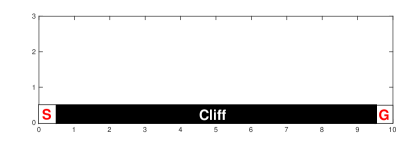
Figure 1: A continuous cliff world. S and G indicate the start and goal position respectively. Moving through the white region induces low cost, while “falling” over the cliff induces very high cost.

In order to formulate this problem as an optimal control problem as defined by Equations (1) and (5), we should replace the hard constraint of the cliff by a soft constraint which penalizes the distance of the mass from the cliff. Thus, we define the following cost function for this problem

$$\Phi_{f}(\mathbf{x})=100(x-10)^{2}+100y^{2}+10(\dot{x}^{2}+\dot{y}^{2})$$ (24)

$$L(t,\mathbf{x},\mathbf{u})=\frac{0.1}{(0.1y+1)^{10}}+u_{x}^{2}+0.01u_{y}^{2}$$ (25)

Equation (24) is the terminal cost at $t_{f}=3$ which puts a high penalty for deviating from the goal state, $[10,0]^{T}$, at time 3[sec]. It also penalizes the point mass speed at the final time. Therefore, the final cost encourages the point mass to reach and stop at the goal state within 3 seconds. In Equation (25), the first term is a penalty term for falling off the cliff. Finally, the last two terms add cost for the exerted control forces in each motion directions. Notice that since the noise in Y direction has higher standard deviation, we penalize the controller less for the effort to confront the noise.

Although the point mass in this problem has linear system dynamics, the defined cost function is nonlinear. Consequently the optimal control problem defined by this cost function is nonlinear. We use ILEG on this problem to find the optimal policy. The algorithm converges after few iterations. The resulting control policy shows different characteristics depending on the chosen parameter $\sigma$. In general, $\sigma$ has an upper limit beyond which the designed policy will be unstable. In this cliff world problem, this limit is 50. Here, we implemented the ILEG algorithm for 5 different choices of $\sigma$.

Figure 2 demonstrates the changes of the feedback gains over time in the Y direction. As expected, by decreasing $\sigma$ from $\sigma=+45$ to $\sigma=-100$ the absolute value of the gains decreases monotonically. For $\sigma=0$, the value of $\sigma$ which the controller does not take the stochasticity of the problem into account (it is the solution to the non exponential cost function). As Figure 2 shows by increasing $\sigma$ to positive values the controller uses higher gains to reduce the variance of the generated motions. However, if we decrease $\sigma$ to negative values, the controller uses lower gains and therefore the motion generated under this controller will have higher variations. In order to compensate for these higher variations which can cause the point mass to fall off the cliff, whereas the $\sigma$-negative controller will choose a more conservative path. In other words, to deal with the uncertainty, the controller prefers a safer plan over a stiffer controller. Figure 3 illustrates this for three different $\sigma$ values.

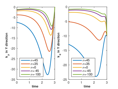
Figure 2: Y direction controller gains for 5 different $\sigma$ values, namely 45, 35, 0, -45, and -100. The left plot illustrates the changes of the proportional gains in the course of time and the right plot shows the derivative gains.

As in Figure 3, the positive $\sigma$ takes a shorter path than the negative one while the negative $\sigma$ chooses a safer path. In this figure the shaded error–bands are a measure of the path variations under the system noise. We see that, since the negative $\sigma$ has lower gains, it has a wider error–band than the positive one.

VII CONCLUSIONS AND FUTURE WORK

In this preliminary work, we have introduced an iterative optimal control algorithm named as ILEG. ILEG iteratively approximates the system dynamics and the cost function by a linear system and an exponential-quadratic cost respectively. Then it efficiently solves the approximated LEG subproblems. We showed that the advantages of using exponential cost function instead of a regular one is that the higher order momenta of the performance index are also considered during the optimization.

An interesting aspect of the ILEG algorithm is that it introduces an algorithmic parameter which can control the behavior of the optimal control. By setting this parameter to zero, ILEG basically reduces to the well-known SLQ. However by setting this parameter to a positive or a negative value, we can obtain two different types of policies. For the positive-value parameter the control policy mostly relies on the error feedback signal, using high gains (’stiff controls’) while in the negative-value parameter the control policy contains a robust plan (forward controls), using lower gains.

VII-A Future Work

This work is currently in its early stage. The effect of the $\sigma$ parameter should be studied through more analytical methods rather than a numerical example. Furthermore, even though Algorithm 1 imposes an upper bound on $\sigma$, it is not totally clear that this is the only restriction over $\sigma$. Questions like the stability of the designed controller under different values of $\sigma$ should be also addressed. Last but not least, the proposed algorithm should be implemented on more practical examples.

VIII ACKNOWLEDGMENTS

This research has been supported in part by a Swiss National Science Foundation Professorship Award to Jonas Buchli, the NCCR Robotics and a Max-Planck ETH Center for Learning Systems Ph.D. fellowship to Farbod Farshidian.

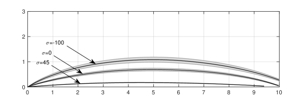
Figure 3: The traversed path of the point mass using controllers with 3 different $\sigma$ values, namely 45, 0, and -100. The shaded area is 15 percent SD of the trajectories

IX Appendix A

Corollary 1: The cost function in Equation (3) can be expanded as

$$\frac{1}{\sigma}\log[J]=\mathbb{E}[\mathcal{J}^{*}]+\frac{\sigma}{2}\mathbb{\mu}_{2}[\mathcal{J}^{*}]+\frac{\sigma^{2}}{6}\mathbb{\mu}_{3}[\mathcal{J}^{*}]+...$$ (26)

where $\mathbb{\mu}_{2}$ and $\mathbb{\mu}_{3}$ are the variance and the skewness of $\mathcal{J^{*}}$ respectively.

Proof: Assuming that the cost associated with one execution of the optimal policy is $\mathcal{J}^{*}$. We can show $J$ as

$$J=\mathbb{E}\left\{\exp[\sigma\mathcal{J}^{*}]\right\}$$ (27)

Therefore we will have

$$\frac{1}{\sigma}\log[J]=\frac{1}{\sigma}\log\mathbb{E}\left\{\exp[\sigma\mathcal{J}^{*}]\right\}$$ (28)

$\log\mathbb{E}\left\{\exp[\sigma\mathcal{J}^{*}]\right\}$ is the cumulant generating function of the random variable $\mathcal{J}^{*}$. By writing the Taylor series expansion of $\log[J]$, we will have

$$\frac{1}{\sigma}\log[J]==\sum_{i=1}^{\infty}{\kappa_{i}\frac{\sigma^{i-1}}{i!}}$$ (29)

where $\kappa_{i}$ is the ith cumulant of $\mathcal{J}$. Using the fact that the first three cumulants are mean, variance, and skewness will conclude the proof.

X Appendix B

Theorem 1: The solution to the optimal control problem defined in Equations (1) and (5) is

$$J=\exp\left[\sigma\Psi(0,\mathbf{x}_{0})\right]$$ (30)

$$\mathbf{u}^{*}(t,\mathbf{x})=\mathbf{R}(t,\mathbf{x})^{-1}\left(\mathbf{r}(t,x)+\mathbf{G}^{T}(t,\mathbf{x})\nabla_{\mathbf{x}}\Psi(t,\mathbf{x})\right)$$ (31)

where $\Psi(t,\mathbf{x})$ is the solution to the following partial differential equation (PDE)

$$-\partial_{t}\Psi=\Phi-\frac{1}{2}\mathbf{r}^{T}\mathbf{R}^{-1}\mathbf{r}+\nabla_{\mathbf{x}}\Psi^{T}\left(\mathbf{f}-\mathbf{G}\mathbf{R}^{-1}\mathbf{r}\right)-\frac{1}{2}\nabla_{\mathbf{x}}\Psi^{T}\big{(}GR^{-1}G^{T}-\sigma\mathbf{C}\Sigma\mathbf{C}^{T}\big{)}\nabla_{\mathbf{x}}\Psi+\frac{1}{2}Tr[\nabla_{\mathbf{x}\mathbf{x}}\Psi\mathbf{C}\Sigma\mathbf{C}^{T}]$$ (32)

with boundary condition $\Psi(t_{f},\mathbf{x})=\Phi_{f}(x)$ (to make the equation shorter, we have dropped the functionality with respect to $t$ and $\mathbf{x}$).

Proof: In order to solve this optimal control problem, we chose a dynamic programming approach. First consider a discrete time problem with the system dynamics described by Equation (33)

$$\mathbf{x}_{n+1}=\mathbf{f}(n,\mathbf{x}_{n})+\mathbf{G}(n,\mathbf{x}_{n})\mathbf{u}_{n}+\mathbf{C}(n,\mathbf{x}_{n})\mathbf{w}_{n}$$ (33)

where $\mathbf{w}_{n}$ is a Gaussian random process with zero mean and covariance $\mathbb{C}ov(\mathbf{w}_{n},\mathbf{w}_{m})=\Sigma\delta_{n,m}$. The discrete cost function is also defined as the following

$$J=\min\limits_{\mathbf{u}_{0}\dots\mathbf{u}_{N-1}}\mathbb{E}\left\{\exp\left[\sigma\left(\Phi(x_{N})+\sum_{n=0}^{N-1}{L(n,\mathbf{x}_{n},\mathbf{u}_{n})}\right)\right]\right\}$$ (34)

It can be easily shown that the solution to this discrete optimal control problem can be obtained using Equation (35).

$$V(n,\mathbf{x})=\min\limits_{\mathbf{u}_{n}}\Big{\{}\exp\left(\sigma L(t,\mathbf{x},\mathbf{u}_{n})\right)\mathbb{E}\left[V(n+1,\mathbf{x}_{n+1})\right]\Big{\}},\qquad V(N,\mathbf{x})=\Phi(\mathbf{x})$$ (35)

This equation is called the extended Bellman equation.

In order to find the solution of the continuous time optimal control problem defined in Equations (1) and (5), we should find the equivalent dynamic programming formula. This can be achieved by discretizing the continuous time equation and using the extended Bellman equation to find the optimality equation. Then by the use of the Ito lemma, we can derive the following optimality equation called extended HJB equation.

$$-\partial_{t}V(t,\mathbf{x})=\min\limits_{\mathbf{u}_{t}}\left\{\sigma V(t,\mathbf{x})L(t,\mathbf{x},\mathbf{u}_{t})+\nabla_{\mathbf{x}}V^{T}(t,\mathbf{x})\left(\mathbf{f}(t,\mathbf{x})+\mathbf{G}(t,\mathbf{x})\mathbf{u}_{t}\right)+\frac{1}{2}Tr[\nabla_{\mathbf{x}\mathbf{x}}V(t,\mathbf{x})\mathbf{C}(t,\mathbf{x}_{t})\Sigma\mathbf{C}^{T}(t,\mathbf{x}_{t})]\right\},\hskip 2.84526ptV(t_{f},\mathbf{x})=\Phi(\mathbf{x})$$ (36)

Using the exponential transformation $V(t,\mathbf{x})=\exp(\sigma\Psi(t,\mathbf{x}))$ in (36) we get

$$V(t,\mathbf{x})=\exp(\sigma\Psi(t,\mathbf{x}))$$ (37)

$$\partial_{t}V(t,\mathbf{x})=\sigma V(t,\mathbf{x})\partial_{t}\Psi(t,\mathbf{x})$$ (38)

$$\nabla_{\mathbf{x}}V(t,\mathbf{x})=\sigma V(t,\mathbf{x})\nabla_{\mathbf{x}}\Psi(t,\mathbf{x})$$ (39)

$$\nabla_{\mathbf{x}\mathbf{x}}V(t,\mathbf{x})=V(t,\mathbf{x})\left(\sigma^{2}\nabla_{\mathbf{x}}\Psi(t,\mathbf{x})\nabla_{\mathbf{x}}\Psi^{T}(t,\mathbf{x})+\sigma\nabla_{\mathbf{x}\mathbf{x}}\Psi(t,\mathbf{x})\right)$$ (40)

Substituting these equations in the extended HJB equation (for the simplicity we will drop all of the subscripts)

$$-\sigma V(t,\mathbf{x})\partial_{t}\Psi(t,\mathbf{x})= \min\limits_{\mathbf{u}_{t}}\Big{\{}\sigma V(t,\mathbf{x})L(t,\mathbf{x},\mathbf{u}_{t})+\sigma V(t,\mathbf{x})\nabla_{\mathbf{x}}\Psi^{T}(t,\mathbf{x})\left(\mathbf{f}(t,\mathbf{x})+\mathbf{G}(t,\mathbf{x})\mathbf{u}_{t}\right)+$$

$$\frac{1}{2}Tr[V(t,\mathbf{x})\left(\sigma^{2}\nabla_{\mathbf{x}}\Psi(t,\mathbf{x})\nabla_{\mathbf{x}}\Psi^{T}(t,\mathbf{x})+\sigma\nabla_{\mathbf{x}\mathbf{x}}\Psi(t,\mathbf{x})\right)\mathbf{C}(t,\mathbf{x}_{t})\Sigma\mathbf{C}^{T}(t,\mathbf{x}_{t})]\Big{\}}$$ (41)

by further simplification we get

$$-\partial_{t}\Psi(t,\mathbf{x})= \min\limits_{\mathbf{u}_{t}}\Big{\{}L(t,\mathbf{x},\mathbf{u}_{t})+\nabla_{\mathbf{x}}\Psi^{T}(t,\mathbf{x})\left(\mathbf{f}(t,\mathbf{x})+\mathbf{G}(t,\mathbf{x})\mathbf{u}_{t}\right)$$

$$+\frac{\sigma}{2}\nabla_{\mathbf{x}}\Psi^{T}(t,\mathbf{x})\mathbf{C}(t,\mathbf{x}_{t})\Sigma\mathbf{C}^{T}(t,\mathbf{x}_{t})\nabla_{\mathbf{x}}\Psi(t,\mathbf{x})+\frac{1}{2}Tr[\nabla_{\mathbf{x}\mathbf{x}}\Psi(t,\mathbf{x})\mathbf{C}(t,\mathbf{x}_{t})\Sigma\mathbf{C}^{T}(t,\mathbf{x}_{t})]\Big{\}}$$ (42)

If we assume that the cost function is quadratic with respect to control input $\mathbf{u}_{t}$ as

$$L(t,\mathbf{x},\mathbf{u}_{t})=\phi(t,\mathbf{x})+\frac{1}{2}\mathbf{u}_{t}^{T}\mathbf{R}(t)\mathbf{u}_{t}+\mathbf{u}_{t}^{T}\mathbf{r}(t,x)$$ (43)

the optimal control input will be

$$\mathbf{u}^{*}(t,\mathbf{x})=-\mathbf{R}(t)^{-1}\left(\mathbf{r}(t,x)+\mathbf{G}^{T}(t,\mathbf{x})\nabla_{\mathbf{x}}\Psi(t,\mathbf{x})\right)$$ (44)

and the HJB equation will be

$$-\partial_{t}\Psi=\phi-\frac{1}{2}\mathbf{r}^{T}\mathbf{R}^{-1}\mathbf{r}+\nabla_{\mathbf{x}}\Psi^{T}\left(\mathbf{f}-\mathbf{G}\mathbf{R}^{-1}\mathbf{r}\right)-\frac{1}{2}\nabla_{\mathbf{x}}\Psi^{T}\left(GR^{-1}G^{T}-\sigma\mathbf{C}\Sigma\mathbf{C}^{T}\right)\nabla_{\mathbf{x}}\Psi+\frac{1}{2}Tr[\nabla_{\mathbf{x}\mathbf{x}}\Psi\mathbf{C}\Sigma\mathbf{C}^{T}]$$ (45)

XI Appendix C

Theorem 2: The solution to the optimal control problem defined in Equations​ (11-17) exists if $\left(\mathbf{B}_{t}\mathbf{R}_{t}^{-1}\mathbf{B}_{t}^{T}-\sigma\mathbf{C}_{t}\Sigma\mathbf{C}_{t}^{T}\right)$ is positive semidefinite for all the ts and the solution can be found as it follows

$$-\dot{\mathbf{S}}_{t}= \mathbf{Q}_{t}+\mathbf{A}_{t}^{T}\mathbf{S}_{t}+\mathbf{S}_{t}^{T}\mathbf{A}_{t}-\left(\mathbf{P}_{t}^{T}+\mathbf{B}_{t}^{T}\mathbf{S}_{t}\right)^{T}\mathbf{R}_{t}^{-1}\left(\mathbf{P}_{t}^{T}+\mathbf{B}_{t}^{T}\mathbf{S}_{t}\right)$$

$$+\sigma\mathbf{S}_{t}^{T}\mathbf{C}_{t}\Sigma\mathbf{C}_{t}^{T}\mathbf{S}_{t}$$ (46)

$$-\dot{\mathbf{s}}_{t}= \mathbf{q}_{t}+\mathbf{A}_{t}^{T}\mathbf{s}_{t}-\left(\mathbf{P}_{t}^{T}+\mathbf{B}_{t}^{T}\mathbf{S}_{t}\right)^{T}\mathbf{R}_{t}^{-1}\left(\mathbf{r}_{t}+\mathbf{B}_{t}^{T}\mathbf{s}_{t}\right)$$

$$+\sigma\mathbf{S}_{t}^{T}\mathbf{C}_{t}\Sigma\mathbf{C}_{t}^{T}\mathbf{s}_{t}$$ (47)

$$-\dot{s}_{t}= q_{t}-\frac{1}{2}\left(\mathbf{r}_{t}+\mathbf{B}_{t}^{T}\mathbf{s}_{t}\right)^{T}\mathbf{R}_{t}^{-1}\left(\mathbf{r}_{t}+\mathbf{B}_{t}^{T}\mathbf{s}_{t}\right)+\frac{1}{2}Tr\left[\mathbf{S}(t)\mathbf{C}_{t}\Sigma\mathbf{C}_{t}^{T}\right]$$

$$+\frac{\sigma}{2}\mathbf{s}_{t}^{T}\mathbf{C}_{t}\Sigma\mathbf{C}_{t}^{T}\mathbf{s}_{t}$$ (48)

with the final values $\mathbf{S}_{t_{f}}=\mathbf{Q}_{f}$, $\mathbf{s}_{t_{f}}=\mathbf{q}_{f}$, and $s_{t_{f}}=q_{f}$. The optimal control is

$$\delta\mathbf{u}^{*}(t,\mathbf{x})=\mathbf{l}(t)+\mathbf{L}(t)\delta\mathbf{x}$$ (49)

$$\mathbf{l}(t)=-\mathbf{R}_{t}^{-1}\left(\mathbf{r}_{t}+\mathbf{B}_{t}^{T}\mathbf{s}_{t}\right)$$ (50)

$$\mathbf{L}(t)=-\mathbf{R}_{t}^{-1}\left(\mathbf{P}_{t}^{T}+\mathbf{B}_{t}^{T}\mathbf{S}_{t}\right)$$ (51)

Proof: The approximate optimal control problem defined in Equations​ (11-17) can be solved by the use of Equation (32). We will make the following Ansatz for $\Psi(t,\delta\mathbf{x})$ to solve PDE

$$\Psi(t,\delta\mathbf{x})=s(t)+\mathbf{s}(t)^{T}\delta\mathbf{x}+\frac{1}{2}\delta\mathbf{x}^{T}\mathbf{S}(t)\delta\mathbf{x}$$ (52)

$$\partial_{t}\Psi(t,\delta\mathbf{x})=\dot{s}(t)+\dot{\mathbf{s}}(t)^{T}\delta\mathbf{x}+\frac{1}{2}\delta\mathbf{x}^{T}\dot{\mathbf{S}}(t)\delta\mathbf{x}$$ (53)

$$\nabla_{\mathbf{x}}\Psi_{\delta x}(t,\delta\mathbf{x})=\mathbf{s}(t)+\mathbf{S}(t)\delta\mathbf{x}$$ (54)

$$\nabla_{\mathbf{x}\mathbf{x}}\Psi_{\delta x\delta x}(t,\delta\mathbf{x})=\mathbf{S}(t)$$ (55)

Then we will have

$$-\dot{s}_{t}-\dot{\mathbf{s}}_{t}^{T}\delta\mathbf{x}-\frac{1}{2}\delta\mathbf{x}^{T}\dot{\mathbf{S}}_{t}\delta\mathbf{x}=q_{t}-\frac{1}{2}\mathbf{r}_{t}^{T}\mathbf{R}_{t}^{-1}\mathbf{r}_{t}+\delta\mathbf{x}^{T}\left(\mathbf{q}_{t}-\mathbf{P}_{t}\mathbf{R}_{t}^{-1}\mathbf{r}_{t}\right)+\frac{1}{2}\delta\mathbf{x}^{T}\left(\mathbf{Q}_{t}-\mathbf{P}_{t}\mathbf{R}_{t}^{-1}\mathbf{P}_{t}^{T}\right)\delta\mathbf{x}$$

$$+\left(\mathbf{s}_{t}+\mathbf{S}_{t}\delta\mathbf{x}\right)^{T}\left(\mathbf{A}_{t}\delta\mathbf{x}-\mathbf{B}_{t}\mathbf{R}_{t}^{-1}\mathbf{r}_{t}-\mathbf{B}_{t}\mathbf{R}_{t}^{-1}\mathbf{P}_{t}^{T}\delta\mathbf{x}\right)-\frac{1}{2}\left(\mathbf{s}_{t}+\mathbf{S}_{t}\delta\mathbf{x}\right)^{T}\left(\mathbf{B}_{t}\mathbf{R}_{t}^{-1}\mathbf{B}_{t}^{T}-\sigma\mathbf{C}_{t}\Sigma\mathbf{C}_{t}^{T}\right)\left(\mathbf{s}_{t}+\mathbf{S}_{t}\delta\mathbf{x}\right)+\frac{1}{2}Tr\left[\mathbf{S}(t)\mathbf{C}_{t}\Sigma\mathbf{C}_{t}^{T}\right]$$ (56)

we can rearrange the above equation as

$$-\dot{s}_{t}-\dot{\mathbf{s}}_{t}^{T}\delta\mathbf{x}-\frac{1}{2}\delta\mathbf{x}^{T}\dot{\mathbf{S}}_{t}\delta\mathbf{x}=$$

$$q_{t}-\frac{1}{2}\mathbf{r}_{t}^{T}\mathbf{R}_{t}^{-1}\mathbf{r}_{t}-\mathbf{s}_{t}^{T}\mathbf{B}_{t}\mathbf{R}_{t}^{-1}\mathbf{r}_{t}-\frac{1}{2}\mathbf{s}_{t}^{T}\left(\mathbf{B}_{t}\mathbf{R}_{t}^{-1}\mathbf{B}_{t}^{T}-\sigma\mathbf{C}_{t}\Sigma\mathbf{C}_{t}^{T}\right)\mathbf{s}_{t}+\frac{1}{2}Tr\left[\mathbf{S}(t)\mathbf{C}_{t}\Sigma\mathbf{C}_{t}^{T}\right]$$

$$+\left(\mathbf{q}_{t}-\mathbf{P}_{t}\mathbf{R}_{t}^{-1}\mathbf{r}_{t}\right)^{T}\delta\mathbf{x}+\mathbf{s}_{t}^{T}\left(\mathbf{A}_{t}-\mathbf{B}_{t}\mathbf{R}_{t}^{-1}\mathbf{P}_{t}^{T}\right)\delta\mathbf{x}-\mathbf{r}_{t}^{T}\mathbf{R}_{t}^{-1}\mathbf{B}_{t}^{T}\mathbf{S}_{t}\delta\mathbf{x}-\mathbf{s}_{t}^{T}\left(\mathbf{B}_{t}\mathbf{R}_{t}^{-1}\mathbf{B}_{t}^{T}-\sigma\mathbf{C}_{t}\Sigma\mathbf{C}_{t}^{T}\right)\mathbf{S}_{t}\delta\mathbf{x}$$

$$+\frac{1}{2}\delta\mathbf{x}^{T}\left(\mathbf{Q}_{t}-\mathbf{P}_{t}\mathbf{R}_{t}^{-1}\mathbf{P}_{t}^{T}\right)\delta\mathbf{x}+\delta\mathbf{x}^{T}\mathbf{S}_{t}^{T}\left(\mathbf{A}_{t}-\mathbf{B}_{t}\mathbf{R}_{t}^{-1}\mathbf{P}_{t}\right)\delta\mathbf{x}-\frac{1}{2}\delta\mathbf{x}^{T}\mathbf{S}_{t}^{T}\left(\mathbf{B}_{t}\mathbf{R}_{t}^{-1}\mathbf{B}_{t}^{T}-\sigma\mathbf{C}_{t}\Sigma\mathbf{C}_{t}^{T}\right)\mathbf{S}_{t}\delta\mathbf{x}$$ (57)

By equating the coefficient of $\delta\mathbf{x}$, we will have the following equations.

$$-\dot{\mathbf{S}}_{t}= \mathbf{Q}_{t}-\mathbf{P}_{t}\mathbf{R}_{t}^{-1}\mathbf{P}_{t}^{T}+\left(\mathbf{A}_{t}-\mathbf{B}_{t}\mathbf{R}_{t}^{-1}\mathbf{P}_{t}^{T}\right)^{T}\mathbf{S}_{t}+\mathbf{S}_{t}^{T}\left(\mathbf{A}_{t}-\mathbf{B}_{t}\mathbf{R}_{t}^{-1}\mathbf{P}_{t}^{T}\right)-\mathbf{S}_{t}^{T}\left(\mathbf{B}_{t}\mathbf{R}_{t}^{-1}\mathbf{B}_{t}^{T}-\sigma\mathbf{C}_{t}\Sigma\mathbf{C}_{t}^{T}\right)\mathbf{S}_{t}$$ (58)

$$-\dot{\mathbf{s}}_{t}= \mathbf{q}_{t}-\mathbf{P}_{t}\mathbf{R}_{t}^{-1}\mathbf{r}_{t}+\left(\mathbf{A}_{t}-\mathbf{B}_{t}\mathbf{R}_{t}^{-1}\mathbf{P}^{T}_{t}\right)^{T}\mathbf{s}_{t}-\mathbf{S}_{t}^{T}\mathbf{B}_{t}\mathbf{R}_{t}^{-1}\mathbf{r}_{t}-\mathbf{S}_{t}^{T}\left(\mathbf{B}_{t}\mathbf{R}_{t}^{-1}\mathbf{B}_{t}^{T}-\sigma\mathbf{C}_{t}\Sigma\mathbf{C}_{t}^{T}\right)\mathbf{s}_{t}$$ (59)

$$-\dot{s}_{t}= q_{t}-\frac{1}{2}\mathbf{r}_{t}^{T}\mathbf{R}_{t}^{-1}\mathbf{r}_{t}-\mathbf{s}_{t}^{T}\mathbf{B}_{t}\mathbf{R}_{t}^{-1}\mathbf{r}_{t}-\frac{1}{2}\mathbf{s}_{t}^{T}\left(\mathbf{B}_{t}\mathbf{R}_{t}^{-1}\mathbf{B}_{t}^{T}-\sigma\mathbf{C}_{t}\Sigma\mathbf{C}_{t}^{T}\right)\mathbf{s}_{t}+\frac{1}{2}Tr\left[\mathbf{S}(t)\mathbf{C}_{t}\Sigma\mathbf{C}_{t}^{T}\right]$$ (60)

with final values

$$\mathbf{S}_{t_{f}}=\mathbf{Q}_{t_{f}},\quad\mathbf{s}_{t_{f}}=\mathbf{q}_{t_{f}},\quad s_{t_{f}}=q_{t_{f}}.$$ (61)

and the optimal control

$$\delta\mathbf{u}^{*}(t,\mathbf{x})=-\mathbf{R}_{t}^{-1}\left(\mathbf{r}_{t}+\mathbf{B}_{t}^{T}\mathbf{s}_{t}\right)-\mathbf{R}_{t}^{-1}\left(\mathbf{P}_{t}^{T}+\mathbf{B}_{t}^{T}\mathbf{S}_{t}\right)\delta\mathbf{x}$$ (62)

These equations will have solutions if $\left(\mathbf{B}_{t}\mathbf{R}_{t}^{-1}\mathbf{B}_{t}^{T}-\sigma\mathbf{C}_{t}\Sigma\mathbf{C}_{t}^{T}\right)$ is positive semidefinite for all t. We can further simplify these equations by regrouping them as

$$-\dot{\mathbf{S}}_{t}= \mathbf{Q}_{t}+\mathbf{A}_{t}^{T}\mathbf{S}_{t}+\mathbf{S}_{t}^{T}\mathbf{A}_{t}-\left(\mathbf{P}_{t}^{T}+\mathbf{B}^{T}\mathbf{S}_{t}\right)^{T}\mathbf{R}_{t}^{-1}\left(\mathbf{P}_{t}^{T}+\mathbf{B}^{T}\mathbf{S}_{t}\right)+\sigma\mathbf{S}_{t}^{T}\mathbf{C}_{t}\Sigma\mathbf{C}_{t}^{T}\mathbf{S}_{t}$$ (63)

$$-\dot{\mathbf{s}}_{t}= \mathbf{q}_{t}+\mathbf{A}_{t}^{T}\mathbf{s}_{t}-\left(\mathbf{P}_{t}^{T}+\mathbf{B}_{t}^{T}\mathbf{S}_{t}\right)^{T}\mathbf{R}_{t}^{-1}\left(\mathbf{r}_{t}+\mathbf{B}_{t}^{T}\mathbf{s}_{t}\right)+\sigma\mathbf{S}_{t}^{T}\mathbf{C}_{t}\Sigma\mathbf{C}_{t}^{T}\mathbf{s}_{t}$$ (64)

$$-\dot{s}_{t}= q_{t}-\frac{1}{2}\left(\mathbf{r}_{t}+\mathbf{B}_{t}^{T}\mathbf{s}_{t}\right)^{T}\mathbf{R}_{t}^{-1}\left(\mathbf{r}_{t}+\mathbf{B}_{t}^{T}\mathbf{s}_{t}\right)+\frac{1}{2}Tr\left[\mathbf{S}(t)\mathbf{C}_{t}\Sigma\mathbf{C}_{t}^{T}\right]+\frac{\sigma}{2}\mathbf{s}_{t}^{T}\mathbf{C}_{t}\Sigma\mathbf{C}_{t}^{T}\mathbf{s}_{t}$$ (65)

References

[1]
D. Mayne, “A second-order gradient method for determining optimal trajectories
of non-linear discrete-time systems,” International Journal of
Control, vol. 3, no. 1, 1966.
[2]
J. Dunn and D. Bertsekas, “Efficient dynamic programming implementations of
newton’s method for unconstrained optimal control problems,” Journal
of Optimization Theory and Applications, vol. 63, no. 1, pp. 23–38, 1989.
[3]
A. Sideris and J. Bobrow, “An efficient sequential linear quadratic algorithm
for solving nonlinear optimal control problems,” Automatic Control,
IEEE Transactions on, vol. 50, no. 12, pp. 2043–2047, 2005.
[4]
E. Todorov and W. Li, “A generalized iterative lqg method for locally-optimal
feedback control of constrained nonlinear stochastic systems,” in
Proc. of the American Control Conference, 2005.
[5]
D. Jacobson, “Optimal stochastic linear systems with exponential performance
criteria and their relation to deterministic differential games,”
Automatic Control, IEEE Transactions on, vol. 18, no. 2, pp. 124–131,
1973.