Gain and loss enhancement in active and passive particulate composite materials

Abstract

Two active dielectric materials may be blended together to realize a homogenized composite material (HCM) which exhibits more gain than either component material. Likewise, two dissipative dielectric materials may be blended together to realize an HCM which exhibits more loss than either component material. Sufficient conditions for such gain/loss enhancement were established using the Bruggeman homogenization formalism. Gain/loss enhancement arises when (i) the imaginary parts of the relative permittivities of both component materials are similar in magnitude and (ii) the real parts of the relative permittivities of both component materials are dissimilar in magnitude.

Keywords: Bruggeman homogenization formalism; active materials; dissipative materials; gain enhancement; loss enhancement

1 Introduction

Two (or more) particulate materials may be mixed together to realize a homogenized composite material (HCM), provided that the particles making up the component materials are much smaller than the wavelengths involved [1]. To be of practical value, an HCM is generally required to exhibit a desirable blend of certain properties of its component materials. Metamaterials are HCMs whose performances exceed those of their component materials [2, 3]. Within the electromagnetic realm, many instances of such HCMs can be found. For examples: through the process of homogenization, the phenomenon of weak nonlinearity may be enhanced [4, 5, 6], and the group speed may be enhanced beyond the maximum group speed in the component materials [7, 8] or weakened below the minimum group speed in the component materials [9].

In this short article, the prospect of enhancing gain by means of homogenization is explored for HCMs arising from active component materials. The dual process of loss enhancement in HCMs arising from dissipative component materials is also considered. The well–established Bruggeman homogenization formalism [10, 11, 12] is employed, all component materials being thereby treated on the same footing. Accordingly, this formalism is applicable for all values of volume fraction of the component materials.

2 Homogenization via the Bruggeman formalism

Let us consider a composite material comprising two distinct materials labelled ‘a’ and ‘b’ that are distributed randomly as electrically small spheres. Both component materials are isotropic dielectric materials with relative permittivities $\varepsilon_{a}=\varepsilon^{r}_{a}+i\varepsilon^{i}_{a}$ and $\varepsilon_{b}=\varepsilon^{r}_{b}+i\varepsilon^{i}_{b}$, respectively, wherein $\varepsilon^{r,i}_{a,b}\in\mathbb{R}$ and $\varepsilon_{a}\neq\varepsilon_{b}$. Physical plausibility requires the imposition of the restriction $\varepsilon^{r}_{a}\varepsilon^{r}_{b}>0$ on the Bruggeman formalism [13].

The Bruggeman estimate $\varepsilon_{Br}=\varepsilon^{r}_{Br}+i\varepsilon^{i}_{Br}$ of the HCM relative permittivity is provided implicitly by the quadratic equation [10]

$$2\varepsilon^{2}_{Br}+\varepsilon_{Br}\left[\varepsilon_{a}\left(1-3f_{a}\right)+\varepsilon_{b}\left(3f_{a}-2\right)\right]-\varepsilon_{a}\varepsilon_{b}=0\,,$$ (1)

with $f_{a}$ being the volume fraction of component material ‘a’. The limiting conditions $\varepsilon_{Br}\to\varepsilon_{b}$ as $f_{a}\to 0$, and $\varepsilon_{Br}\to\varepsilon_{a}$ as $f_{a}\to 1$ allow the correct root to be extracted from Eq. (1).

When both component materials are active (i.e., $\varepsilon^{i}_{a,b}<0$), the phenomenon of gain enhancement is signified by $\varepsilon^{i}_{Br}<\min\left\{\varepsilon^{i}_{a},\varepsilon^{i}_{b}\right\}$. When both component materials are dissipative (i.e., $\varepsilon^{i}_{a,b}>0$), the phenomenon of loss enhancement is signified by $\varepsilon^{i}_{Br}>\max\left\{\varepsilon^{i}_{a},\varepsilon^{i}_{b}\right\}$.

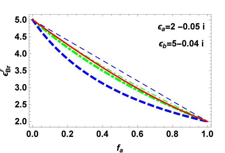
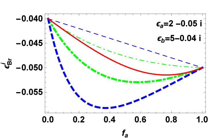
Figure 1: The real and imaginary parts of the HCM relative permittivity $\varepsilon_{Br}$ estimated by the Bruggeman formalism (red, solid curves) plotted against volume fraction $f_{a}$, when $\varepsilon_{a}=2-0.05i$ and $\varepsilon_{a}=5-0.04i$. Also plotted are the Hashin–Shtrikman bounds: $\mbox{HS}_{\alpha}$ (thin, green, broken dashed curves) and $\mbox{HS}_{\beta}$ (thick, green, broken dashed curves); and the Wiener bounds: $\mbox{W}_{\alpha}$ (thin, blue, dashed curves) and $\mbox{W}_{\beta}$ (thick, blue, dashed curves).

To illustrate the phenomenon of gain enhancement, let us consider a specific example. Suppose that the component materials are active ones, specified by $\varepsilon_{a}=2-0.05i$ and $\varepsilon_{b}=5-0.04i$. The real and imaginary parts of the Bruggeman estimate of the HCM relative permittivity are plotted against volume fraction in Fig. 1. Also plotted in this figure are two well–established bounds on the HCM relative permittivity, namely the Wiener bounds [14]

$$\left.\begin{array}[]{l}\mbox{W}_{\alpha}=f_{a}\varepsilon_{a}+f_{b}\varepsilon_{b}\vspace{8pt}\\ \mbox{W}_{\beta}=\displaystyle{\left(\frac{f_{a}}{\varepsilon_{a}}+\frac{f_{b}}{\varepsilon_{b}}\right)^{-1}}\end{array}\right\}\,$$ (2)

and the Hashin–Shtrikman bounds [15]

$$\left.\begin{array}[]{l}\displaystyle{\mbox{HS}_{\alpha}=\varepsilon_{b}+\frac{3f_{a}\varepsilon_{b}\left(\varepsilon_{a}-\varepsilon_{b}\right)}{\varepsilon_{a}+2\varepsilon_{b}-f_{a}\left(\varepsilon_{a}-\varepsilon_{b}\right)}\vspace{8pt}}\\ \displaystyle{\mbox{HS}_{\beta}=\varepsilon_{a}+\frac{3f_{b}\varepsilon_{a}\left(\varepsilon_{b}-\varepsilon_{a}\right)}{\varepsilon_{b}+2\varepsilon_{a}-f_{b}\left(\varepsilon_{b}-\varepsilon_{a}\right)}}\end{array}\right\}\,.$$ (3)

Herein, $f_{b}=1-f_{a}$ is the volume fraction of component material ‘b’. Originally, the Wiener bounds and the Hashin–Shtrikman bounds were derived for HCMs characterized by wholly real–valued constitutive parameters, but generalizations to complex–valued constitutive parameters later emerged [16].

The Hashin–Shtrikman bound $\mbox{HS}_{\alpha}$ is equivalent to the Maxwell Garnett estimate of the HCM relative permittivity, based on the homogenization of a random dispersal of spheres of component material ‘a’ embedded in the host component material ‘b’, valid for $f_{a}\lesssim 0.3$ [17]. Similarly, $\mbox{HS}_{\beta}$ is equivalent to the Maxwell Garnett estimate of the HCM relative permittivity, based on the homogenization of a random dispersal of spheres of component material ‘b’ embedded in the host component material ‘a’, valid for $f_{b}\lesssim 0.3$.

The real part of $\varepsilon_{Br}$ is seen in Fig. 1 to decrease uniformly from $\varepsilon^{r}_{b}$ to $\varepsilon^{r}_{a}$ as $f_{a}$ increases from $0$ to $1$. Furthermore, $\varepsilon^{r}_{Br}$ is tightly bounded by $\mbox{HS}_{\alpha}$ and $\mbox{HS}_{\beta}$, and less tightly bounded by $W_{\alpha}$ and $W_{\beta}$. The imaginary part of $\varepsilon_{Br}$ follows a more interesting trajectory as $f_{a}$ increases: $\varepsilon^{i}_{Br}$ decreases from $\varepsilon^{i}_{b}$ at $f_{a}=0$, reaches a minimum value at $f_{a}\approx 0.8$, and then increases to reach $\varepsilon^{i}_{a}$ at $f_{a}=1$. Thus, according to the Bruggeman formalism, gain enhancement arises in the vicinity of $f_{a}\approx 0.8$, with the minimum value of $\varepsilon^{i}_{Br}$ ($\approx-0.0515$) being approximately $3\%$ smaller than $\min\left\{\varepsilon^{i}_{a},\varepsilon^{i}_{b}\right\}$. Furthermore, ${\rm Im}\left(\mbox{HS}_{\beta}\right)<\min\left\{\varepsilon^{i}_{a},\varepsilon^{i}_{b}\right\}$ when $0.7\lesssim f_{a}<1$. Thus, gain enhancement is also predicted by the Maxwell Garnett formalism.

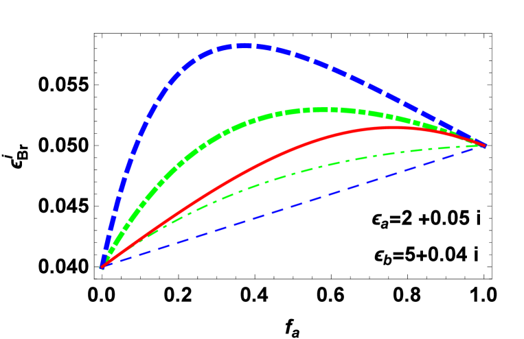
Figure 2: As Fig. 1 except that both component materials are dissipative, having the relative permittivities $\varepsilon_{a}=2+0.05i$ and $\varepsilon_{a}=5+0.04i$.

Loss enhancement mirrors gain enhancement. To support this assertion, let us consider the dissipative counterpart of the active HCM considered in Fig. 1. In Fig. 2, plots are presented which are equivalent to those presented in Fig. 1 but now the component materials are dissipative ones, specified by $\varepsilon_{a}=2+0.05i$ and $\varepsilon_{b}=5+0.04i$. As in Fig. 1, $\varepsilon_{Br}^{r}$ in Fig. 2 decreases uniformly from $\varepsilon^{r}_{b}$ to $\varepsilon^{r}_{a}$ as $f_{a}$ increases from $0$ to $1$; moreover, $\varepsilon^{r}_{Br}$ is tightly bounded by $\mbox{HS}_{\alpha}$ and $\mbox{HS}_{\beta}$, and less tightly bounded by $W_{\alpha}$ and $W_{\beta}$. The plot of $\varepsilon_{Br}^{i}$ in Fig. 2 displays loss enhancement with the maximum value of $\varepsilon^{i}_{Br}$ ($\approx 0.0515$) being approximately $3\%$ larger than $\max\left\{\varepsilon^{i}_{a},\varepsilon^{i}_{b}\right\}$. In addition, ${\rm Im}\left(\mbox{HS}_{\beta}\right)>\max\left\{\varepsilon^{i}_{a},\varepsilon^{i}_{b}\right\}$ when $0.7\lesssim f_{a}<1$. Thus, loss enhancement is predicted by both the Bruggeman formalism and the Maxwell Garnett formalism.

Since the active and dissipative scenarios effectively represent two different sides of the same coin, henceforth in this section we focus on gain enhancement. Let us now turn to the gain–enhancement index

$$\rho=\frac{\varepsilon^{i}_{Br}}{\min\left\{\varepsilon^{i}_{a},\varepsilon^{i}_{b}\right\}}$$ (4)

estimated using the Bruggeman formalism. Gain enhancement is signified by $\rho>1$. For $\varepsilon^{r}_{a}=2$, $\varepsilon^{r}_{b}=5$, and $\varepsilon^{i}_{b}=-0.04$, $\rho$ is plotted against volume fraction $f_{a}$ and the ratio $\varepsilon^{i}_{a}/\varepsilon^{i}_{b}$ in Fig. 3. Gain enhancement is evident for mid–ranges value of $f_{a}$ when $\varepsilon^{i}_{a}/\varepsilon^{i}_{b}\simeq 1$. Specifically for this particular example,

• $\rho$ is as high as about $1.05$, with its maximum value occurring for $f_{a}\approx 0.6$ and $\varepsilon^{i}_{a}/\varepsilon^{i}_{b}=1$; and

• there is no gain enhancement for $\varepsilon^{i}_{a}/\varepsilon^{i}_{b}\lesssim 0.95$ and for $\varepsilon^{i}_{a}/\varepsilon^{i}_{b}\gtrsim 1.07$, regardless of the value of $f_{a}$.

The dependency of $\rho$ upon $\varepsilon_{a}^{r}$ and $\varepsilon_{b}^{r}$ is delineated in Fig. 4, wherein $\rho$ is plotted against $f_{a}$ and $\varepsilon^{r}_{a}/\varepsilon^{r}_{b}$ for $\varepsilon^{i}_{a}=-0.05$, $\varepsilon^{i}_{b}=-0.04$, and $\varepsilon^{r}_{b}=5$. As in Fig. 3, $\rho$ is high for mid-range values of $f_{a}$ when the ratio $\varepsilon^{r}_{a}/\varepsilon^{r}_{b}$ deviates most from unity in Fig. 4. Specifically for this particular example,

• $\rho$ is as high as about $1.4$, with its maximum value occurring for $f_{a}\approx 0.7$ and $\varepsilon^{r}_{a}/\varepsilon^{r}_{b}=0.1$;

• $\rho$ is as high as about $1.2$, with its maximum value occurring for $f_{a}\approx 0.5$ and $\varepsilon^{r}_{a}/\varepsilon^{r}_{b}=10$; and

• there is no gain enhancement for $\varepsilon^{r}_{a}/\varepsilon^{r}_{b}\approx 1$, regardless of the value of $f_{a}$.

3 Conditions for gain/loss enhancement

The foregoing and similar calculations led us to conclude that gain enhancement should be expected when

• $\varepsilon^{i}_{a}<0$ and $\varepsilon^{i}_{b}<0$,

• the ratio $\varepsilon^{i}_{a}/\varepsilon^{i}_{b}$ is close to unity, and

• the ratio $\varepsilon^{r}_{a}/\varepsilon^{r}_{b}$ is either very small or very large.

Loss enhancement should be expected when $\varepsilon^{i}_{a}>0$, $\varepsilon^{i}_{b}>0$, and the conditions (ii) and (iii) are satisfied. In order to formally establish this understanding soundly, we used the Bruggeman equation (1) to obtain the gradient

$$\frac{d\varepsilon_{Br}}{df_{a}}=\frac{3\varepsilon_{Br}\left(\varepsilon_{a}-\varepsilon_{b}\right)}{4\varepsilon_{Br}+\varepsilon_{a}\left(1-3f_{a}\right)+\varepsilon_{b}\left(3f_{a}-2\right)}\,.$$ (5)

This expression underlies further analysis.

3.1 Gain enhancement

Suppose that both component materials are active, i.e., $\varepsilon^{i}_{a}<0$ and $\varepsilon^{i}_{b}<0$. If $\varepsilon^{i}_{a}\geq\varepsilon^{i}_{b}$, then a sufficient condition for gain enhancement is that the gradient

$$\lim_{f_{a}\to 0}\frac{d\varepsilon^{i}_{Br}}{df_{a}}<0\,.$$ (6)

Given that

$$\lim_{f_{a}\to 0}\varepsilon_{Br}=\varepsilon_{b}\,,$$ (7)

Eq. (5) yields

$$\lim_{f_{a}\to 0}\frac{d\varepsilon^{i}_{Br}}{df_{a}}=\frac{3\varepsilon_{b}\left(\varepsilon_{a}-\varepsilon_{b}\right)}{2\varepsilon_{b}+\varepsilon_{a}}\,,$$ (8)

and hence

$$\lim_{f_{a}\to 0}\frac{d\varepsilon^{i}_{Br}}{df_{a}}=\frac{3\left\{\left[\varepsilon^{i}_{b}\left(\varepsilon^{r}_{a}-\varepsilon^{r}_{b}\right)+\varepsilon^{r}_{b}\left(\varepsilon^{i}_{a}-\varepsilon^{i}_{b}\right)\right]\left(2\varepsilon^{r}_{b}+\varepsilon_{a}^{r}\right)-\left[\varepsilon^{r}_{b}\left(\varepsilon^{r}_{a}-\varepsilon^{r}_{b}\right)-\varepsilon^{i}_{b}\left(\varepsilon^{i}_{a}-\varepsilon^{i}_{b}\right)\right]\left(2\varepsilon^{i}_{b}+\varepsilon^{i}_{a}\right)\right\}}{\left(2\varepsilon^{r}_{b}+\varepsilon_{a}^{r}\right)^{2}+\left(2\varepsilon^{i}_{b}+\varepsilon^{i}_{a}\right)^{2}}\,.$$ (9)

The sufficient condition (6) for gain enhancement is therefore logically equivalent to

$$\left[\varepsilon^{i}_{b}\left(\varepsilon^{r}_{a}-\varepsilon^{r}_{b}\right)+\varepsilon^{r}_{b}\left(\varepsilon^{i}_{a}-\varepsilon^{i}_{b}\right)\right]\left(2\varepsilon^{r}_{b}+\varepsilon_{a}^{r}\right)<\left[\varepsilon^{r}_{b}\left(\varepsilon^{r}_{a}-\varepsilon^{r}_{b}\right)-\varepsilon^{i}_{b}\left(\varepsilon^{i}_{a}-\varepsilon^{i}_{b}\right)\right]\left(2\varepsilon^{i}_{b}+\varepsilon^{i}_{a}\right)\,.$$ (10)

If $\varepsilon^{i}_{b}\geq\varepsilon^{i}_{a}$ then a sufficient condition for gain enhancement is that the gradient

$$\lim_{f_{a}\to 1}\frac{d\varepsilon^{i}_{Br}}{df_{a}}>0\,.$$ (11)

Following the same argument as used to derive condition (10), we found that the sufficient condition (11) for gain enhancement is logically equivalent to

$$\left[\varepsilon^{i}_{a}\left(\varepsilon^{r}_{a}-\varepsilon^{r}_{b}\right)+\varepsilon^{r}_{a}\left(\varepsilon^{i}_{a}-\varepsilon^{i}_{b}\right)\right]\left(2\varepsilon^{r}_{a}+\varepsilon_{b}^{r}\right)>\left[\varepsilon^{r}_{a}\left(\varepsilon^{r}_{a}-\varepsilon^{r}_{b}\right)-\varepsilon^{i}_{a}\left(\varepsilon^{i}_{a}-\varepsilon^{i}_{b}\right)\right]\left(2\varepsilon^{i}_{a}+\varepsilon^{i}_{b}\right).$$ (12)

The special case $\varepsilon^{i}_{a}=\varepsilon^{i}_{b}$ is noteworthy. Both the conditions (10) and (12) then reduce to

$$\left(\varepsilon^{r}_{a}-\varepsilon^{r}_{b}\right)^{2}>0.$$ (13)

Since condition (13) is always satisfied because $\varepsilon_{a}\neq\varepsilon_{b}$, gain enhancement is guaranteed for all values of $\varepsilon^{r}_{a}$ and $\varepsilon^{r}_{b}$, provided that $\varepsilon^{i}_{a}=\varepsilon^{i}_{b}$.

3.2 Loss enhancement

Suppose both component materials are dissipative, i.e., $\varepsilon^{i}_{a}>0$ and $\varepsilon^{i}_{b}>0$. If $\varepsilon^{i}_{a}\leq\varepsilon^{i}_{b}$, then a sufficient condition for loss enhancement is that the gradient

$$\lim_{f_{a}\to 0}\frac{d\varepsilon^{i}}{df_{a}}>0\,,$$ (14)

which, in the manner described in §3.1, is logically equivalent to the condition

$$\left[\varepsilon^{i}_{b}\left(\varepsilon^{r}_{a}-\varepsilon^{r}_{b}\right)+\varepsilon^{r}_{b}\left(\varepsilon^{i}_{a}-\varepsilon^{i}_{b}\right)\right]\left(2\varepsilon^{r}_{b}+\varepsilon_{a}^{r}\right)>\left[\varepsilon^{r}_{b}\left(\varepsilon^{r}_{a}-\varepsilon^{r}_{b}\right)-\varepsilon^{i}_{b}\left(\varepsilon^{i}_{a}-\varepsilon^{i}_{b}\right)\right]\left(2\varepsilon^{i}_{b}+\varepsilon^{i}_{a}\right)\,.$$ (15)

If $\varepsilon^{i}_{b}\leq\varepsilon^{i}_{a}$, then a sufficient condition for loss enhancement is that the gradient

$$\lim_{f_{a}\to 1}\frac{d\varepsilon^{i}}{df_{a}}<0\,,$$ (16)

which is logically equivalent to the condition

$$\left[\varepsilon^{i}_{a}\left(\varepsilon^{r}_{a}-\varepsilon^{r}_{b}\right)+\varepsilon^{r}_{a}\left(\varepsilon^{i}_{a}-\varepsilon^{i}_{b}\right)\right]\left(2\varepsilon^{r}_{a}+\varepsilon_{b}^{r}\right)<\left[\varepsilon^{r}_{a}\left(\varepsilon^{r}_{a}-\varepsilon^{r}_{b}\right)-\varepsilon^{i}_{a}\left(\varepsilon^{i}_{a}-\varepsilon^{i}_{b}\right)\right]\left(2\varepsilon^{i}_{a}+\varepsilon^{i}_{b}\right)\,.$$ (17)

As in §3.1, both conditions (15) and (17) reduce to condition (13) for the special case $\varepsilon^{i}_{a}=\varepsilon^{i}_{b}$. Therefore, loss enhancement is guaranteed for all values of $\varepsilon^{r}_{a}$ and $\varepsilon^{r}_{b}$ when $\varepsilon^{i}_{a}=\varepsilon^{i}_{b}$.

3.3 Numerical illustration

The conditions (10) and (12) provide a convenient means of exploring the parameter space of the relative permittivities of the component materials that support gain enhancement, and conditions (15) and (17) play the same role for loss enhancement. Let us illustrate this assertion with a numerical example.

In Fig. 5, the parameter spaces that support gain enhancement are mapped for: (i) $\left(-\varepsilon^{i}_{a},-\varepsilon^{i}_{b}\right)\in\left(0,1\right)\times\left(0,1\right)$ with $\varepsilon^{r}_{a}=2$ and $\varepsilon^{r}_{b}=5$; and (ii) $\left(\varepsilon^{r}_{a},\varepsilon^{r}_{b}\right)\in\left(0.5,10\right)\times\left(0.5,10\right)$ with $\varepsilon^{i}_{a}=-0.05$ and $\varepsilon^{r}_{b}=-0.04$. For $\varepsilon^{r}_{a}=2$ and $\varepsilon^{r}_{b}=5$, the gain-enhancement subspace in the $\left(-\varepsilon^{i}_{a},-\varepsilon^{i}_{b}\right)$ space is a window that contains $\varepsilon^{i}_{a}=\varepsilon^{i}_{b}$ and becomes narrower as the magnitudes of $\varepsilon^{i}_{a}$ and $\varepsilon^{i}_{b}$ are decreased. For $\varepsilon^{i}_{a}=-0.05$ and $\varepsilon^{i}_{b}=-0.04$, two gain-enhancement subspaces in the $\left(\varepsilon^{r}_{a},\varepsilon^{R}_{b}\right)$ space exist where $\varepsilon^{r}_{a}$ and $\varepsilon^{r}_{b}$ are dissimilar in magnitude with greater scope for gain enhancement arising when the magnitudes of $\varepsilon^{r}_{a}$ and $\varepsilon^{r}_{b}$ are increased. These trends gleaned from Fig. 5 are wholly consistent with those evident in Figs. 3 and 4.

3.4 Non-dissipative and non-active component materials

In passing, let us remark on the special case when both component materials are neither dissipative nor active, i.e., $\varepsilon^{i}_{a}=\varepsilon^{i}_{b}=0$. Provided that the possibility $\varepsilon_{Br}=0$ is excluded from consideration (which is not physically plausible for the situation $\varepsilon_{a}\varepsilon_{b}>0$ considered here), we infer from Eq. (5) that $\displaystyle{{d\varepsilon_{Br}}/{df_{a}}\neq 0}$. Therefore, $\varepsilon_{Br}$ is either a uniformly increasing or a uniformly decreasing function of $f_{a}$. Hence, $\varepsilon_{Br}$ must lie between $\varepsilon_{a}$ and $\varepsilon_{b}$ for all values of $f_{a}\in[0,1]$.

4 Closing remarks

Using the Bruggeman formalism, we have established in the foregoing sections that an HCM comprising two active (resp. dissipative) component materials may exhibit more gain (resp. loss) than either of its component materials. For the range of $\varepsilon_{a}$ and $\varepsilon_{b}$ values explored in numerical examples here, gain enhancements of up to 40% were found. Furthermore, sufficient conditions for such gain enhancement and loss enhancement have been established in conditions (10) and (12), and (15) and (17), respectively. These enhancements arise when (i) the imaginary parts of the relative permittivities of both component materials are similar in magnitude and (ii) the real parts of the relative permittivities of both component materials are dissimilar in magnitude. Similar gain/loss enhancements also emerge from the Maxwell Garnett formalism for dilute composite materials.

The reported phenomenons of gain enhancement and loss enhancement are likely to be exacerbated by directional effects in anisotropic HCMs, as has been established for nonlinearity enhancement [18, 19] and group-velocity enhancement [20].

Acknowledgments: TGM acknowledges the support of EPSRC grant EP/M018075/1. AL thanks the Charles Godfrey Binder Endowment at Penn State for ongoing financial support of his research activities.

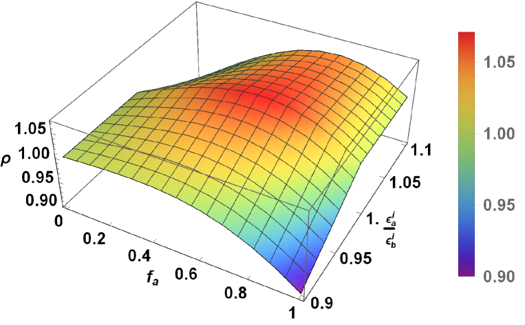
Figure 3: The gain–enhancement index $\rho$ plotted against $f_{a}\in[0,1]$ and $\varepsilon^{i}_{a}/\varepsilon^{i}_{b}\in[0.9,1.1]$, when $\varepsilon^{r}_{a}=2$, $\varepsilon^{r}_{b}=5$, and $\varepsilon^{i}_{b}=-0.04$.

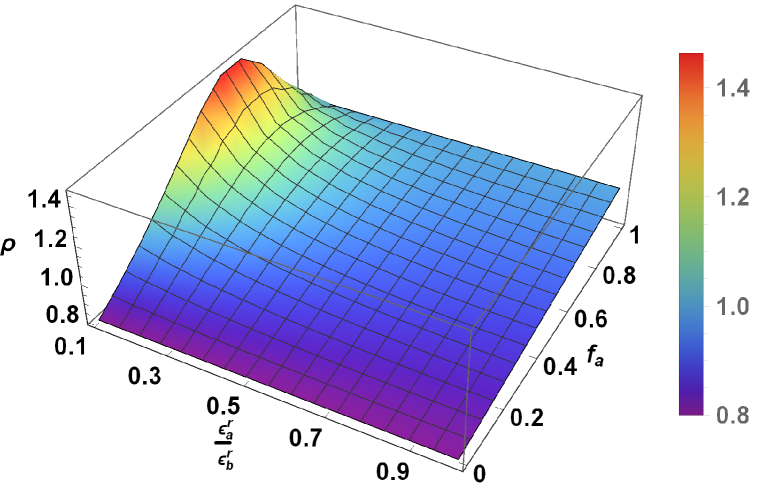
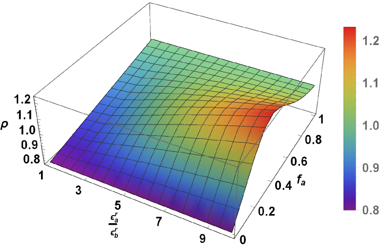
Figure 4: The gain–enhancement index $\rho$ plotted against $f_{a}\in[0,1]$ and $\varepsilon^{r}_{a}/\varepsilon^{r}_{b}\in[0.9,1]\cup[1,10]$, when $\varepsilon^{i}_{a}=-0.05$, $\varepsilon^{i}_{b}=-0.04$, and $\varepsilon^{r}_{b}=5$.

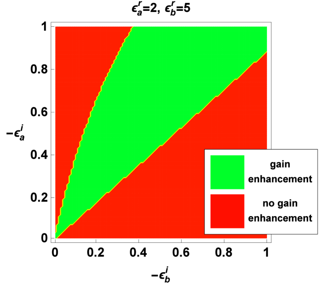
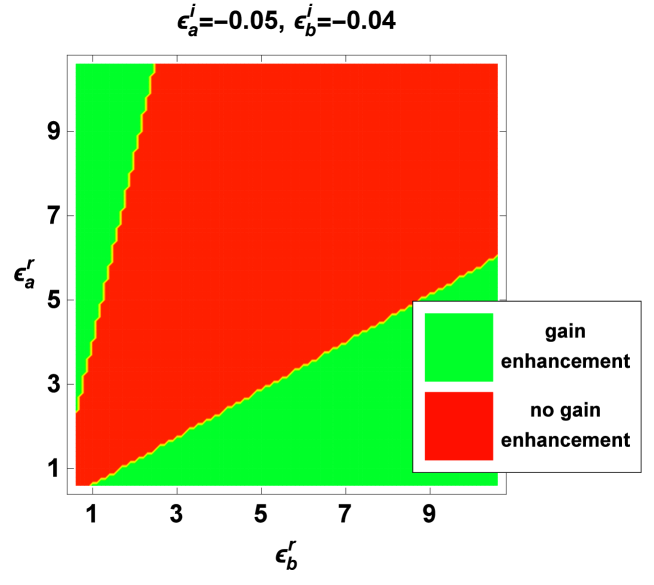
Figure 5: Top: Gain-enhancement subspace in the $\left(-\varepsilon^{i}_{a},-\varepsilon^{i}_{b}\right)$ space, when $\varepsilon^{r}_{a}=2$ and $\varepsilon^{r}_{b}=5$. Bottom: Gain-enhancement subspaces in the $\left(\varepsilon^{r}_{a},\varepsilon^{r}_{b}\right)$ space, when with $\varepsilon^{i}_{a}=-0.05$ and $\varepsilon^{r}_{b}=-0.04$.

References

- [1] Lakhtakia A (ed.). Selected papers on linear optical composite materials. Bellingham (WA): SPIE Optical Engineering Press; 1996.
- [2] Walser RM. Metamaterials: an introduction. In: Introduction to complex mediums for optics and electromagnetics. (W.S. Weiglhofer and A. Lakhtakia, eds). Bellingham (WA): SPIE Press; 2003, pp. 295–316.
- [3] Cui TJ, Smith D, and Liu R (eds.). Metamaterials: theory, design, and applications. New York (NY): Springer; 2010.
- [4] Boyd RW, Gehr RJ, Fischer GL, and Sipe JE. Nonlinear optical properties of nanocomposite materials. Pure Appl. Opt. 1996;5:505–512.
- [5] Liao HB, Xiao RF, Wang H, Wong KS, and Wong GKL. Large third–order optical nonlinearity in composite films measured on a femtosecond time scale. Appl. Phys. Lett. 1998;72:1817–1819.
- [6] Lakhtakia A. Application of strong permittivity fluctuation theory for isotropic, cubically nonlinear, composite mediums. Opt. Commun. 2001;192:145–151.
- [7] Sølna K and Milton GW. Can mixing materials make electromagnetic signals travel faster? SIAM J. Appl. Math. 2002;62:2064–2091.
- [8] Mackay TG and Lakhtakia A. Enhanced group velocity in metamaterials. J. Phys. A: Math. Gen. 2004;37:L19–L24.
- [9] Gao L. Decreased group velocity in compositionally graded films. Phys. Rev. E 2006;73:036602.
- [10] Bruggeman DAG. Berechnung verschiedener physikalischer Konstanten von heterogenen Substanzen, I. Dielektrizitätskonstanten und Leitfähigkeiten der Mischkörper aus isotropen Substanzen. Ann. Phys. Lpz. 1935;24:636–679. (Reproduced in [1]).
- [11] Aspnes DE. Local–field effects and effective–medium theory: a microscopic perspective. Am. J. Phys. 1982;50:704–709. (Reproduced in [1]).
- [12] Mackay TG and Lakhtakia A. Modern analytical electromagnetic homogenization. Bristol (UK): IOP Publishing; 2015.
- [13] Mackay TG and Lakhtakia A. A limitation of the Bruggeman formalism for homogenization. Opt. Commun. 2004;234:35–42. Erratum 2009;282:4028.
- [14] Wiener O. Die Theorie des Mischkörpers für das Feld der Stationären Strömung. Abh. Math.–Phys. Kl. Sächs. 1912;32:507–604. (Reproduced in [1], which also provides an English synopsis of [14] by B. Michel).
- [15] Hashin Z and Shtrikman S. A variational approach to the theory of the effective magnetic permeability of multiphase materials. J. Appl. Phys. 1962;33:3125–3131.
- [16] Milton GW. Bounds on the complex dielectric constant of a composite material. Appl. Phys. Lett. 1980;37:300–302.
- [17] Maxwell Garnett JC. Colours in metal glasses and in metallic films. Phil. Trans. R. Soc. Lond. A 1904;203:385–420. (Reproduced in [1]).
- [18] Lakhtakia MN and Lakhtakia A. Anisotropic composite materials with intensity–dependent permittivity tensor: the Bruggeman approach. Electromagnetics 2001;21:129–138.
- [19] Mackay TG. Geometrically derived anisotropy in cubically nonlinear dielectric composites. J. Phys. D: Appl. Phys. 2003;36:583–591.
- [20] Mackay TG and Lakhtakia A. Anisotropic enhancement of group velocity in a homogenized dielectric composite medium. J. Opt. A: Pure Appl. Opt. 2005:7;669–674.