Calibration of wavefront distortion in light modulator setup by Fourier analysis of multi-beam interference

Abstract

We present a method to calibrate wavefront distortion of the spatial light modulator setup by registering far field images of several Gaussian beams diffracted off the modulator. The Fourier transform of resulting interference images reveals phase differences between typically 5 movable points on the modulator. Repeating this measurement yields wavefront surface. Next, the amplitude efficiency is calibrated be registering near field image. As a verification we produced a superposition of 7th and 8th Bessel beams with different phase velocities and observed their interference.

I Introduction

Phase only spatial light modulator (SLM) finds numerous applications including optical tweezers tweezer ; tweezer2 ; tweezer3 , microscopy mmm ; spiral ; isotripic , or manipulation of atoms bose-einstein ; dynamic ; key-2 . Typically in addition to voltage-controlled phase delay the diffracted beam is subject to wavefront distortion due to SLM curvature, wavefront error of the illuminating beam and possibly the optics between the SLM and final plane of application. The SLM curvature can be calibrated using surface metrology interferometers twyman-green ; zernike . It is more useful however to calibrate the wavefront at the output of the entire setup. This is possible using for example Shack-Hartmann method schack-hartman which measures phase profile gradient or using iterative Gerchberg-Saxon algorithm GS-alg_vortex ; GS-alg which is unfortunately sensitive to starting data and requires rather high dynamic range. Recently methods which aim directly at achieving perfect focusing have been developed nature ; po_nature . They rely on activating two regions on the SLM and observing the interference between two light bundles produced this way. This can be done on a camera po_nature or even using fluorescent-particle nature . The entire wavefront can be reconstructed by scanning one of the regions across the whole SLM.

Here we propose an alternative method for reconstructing wavefront in a particular optical setup involving SLM. To achieve higher throughput and noise immunity we use several regions on the SLM simultaneously and analyze resulting interference images by Fourier transform to extract phase differences. By displaying a number of small phase gratings we diffract parallel beams which focus and interfere together on a far field camera. In addition we correct for nonuniform illumination of the SLM by registering the near field image of diffracted beam.

Our method works with any setup sufficient for registering both near and far field images of diffracted beams. The implementation presented here bases entirely on singlet lenses and enables diagnosing global wavefront properties with any controlled-exposure digital camera placed in the far field. We use second near field camera for an amplitude calibration but even without it full calibration can be accomplished.

This paper is organized as follow. Section II describes the calibration setup. Section III details using phase grating to diffract arbitrary beam. Section IV presents a method to retrieve wavefront distortion from interference of multiple Gaussian beams in Fourier plane. Section V details the amplitude calibration process. Finally section VI describes the way of using a calibrated SLM and presents several methods to verify the calibration.

II Experimental Setup

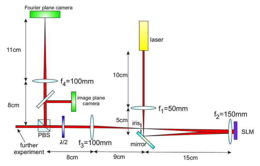
Figure 1: Setup for producing arbitrary beams and calibrating SLM. Lenses $\textnormal{f}_{1}$ and $\textnormal{f}_{2}$ form a telescope to illuminate entire SLM. Iris is used to filter out only 1st order diffracted light. $\textnormal{f}_{2}$ and $\textnormal{f}_{3}$ create SLM image on image plane camera and rely the beam to further experiment. Lens $\textnormal{f}_{4}$ focuses the beam for analyzing far field interference.

The experimental setup is shown in Fig. 1. We use reflective PLUTO SLM from Holoeye (LCOS type with $1920\times 1080$ resolution and 8 $\mu m$ pixel size) and laser with wavelength of 780 $nm$. The beam of illuminating laser is enlarged by a Keplerian telescope consisting of the lenses $\textnormal{f}_{1}$ and $\textnormal{f}_{2}$ in order to illuminate the whole SLM surface. Light reflected and diffracted from the SLM is refocused by $\textnormal{f}_{2}$ lens but only first order diffraction is passed through an iris. Lenses $\textnormal{f}_{3}$ and $\textnormal{f}_{4}$ rely far field from iris plane to the Fourier plane camera, while $\textnormal{f}_{2}$ and $\textnormal{f}_{3}$ create SLM image on image plane camera (resolution 1392 $\times$ 1040, pixel size 6.45 $\mu$m, Bassler sca1400-17fm ). The half wave plate enables adjusting the splitting ratio between diagnostic part and further experiment part.

III Depth-modulated grating

Diffraction of beam with arbitrary amplitude and phase is possible by displaying depth-modulated phase diffraction grating $\Psi(x,y)$ on the SLM. The grating is composed of tiles with depth $a$ and spatial period $d$ and can be described by a formula:

$$\Psi(x,y)=aQ_{d}(x),\quad Q_{d}(x)=2\pi\frac{x}{d}\textnormal{ mod }2\pi.$$ (1)

Let the grating be illuminated with a plane wave of amplitude $E_{0}$. Then the electric field corresponding to the first order diffraction off the grating on SLM plane is:

$$E_{1}(x,y)=E_{0}\textnormal{ sinc}(\pi(1-a))e^{-i\pi(1-a)}e^{i\frac{2\pi}{d}x}$$ (2)

By adjusting the grating depth $a$ and shifting it laterally the amplitude and phase of the diffracted beam can be changed at will. By composing many short fragments of varying depths next to one another, as illustrated in Fig. 2 beam with arbitrary amplitude distribution can be diffracted grating1 ; grating2 . It is necessary for the amplitude of desired diffracted beam to change slowly compared to spatial period of the grating $d$ so that various orders of diffraction can be separated by spatial filtering.

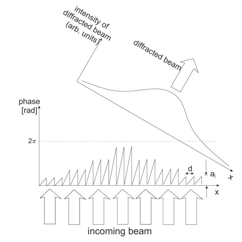
Figure 2: Cross section through a variable-depth phase grating $\Psi(x,y)$ used to diffract beam with arbitrary amplitude. It consists of many fragments with different depths $a_{i}$.

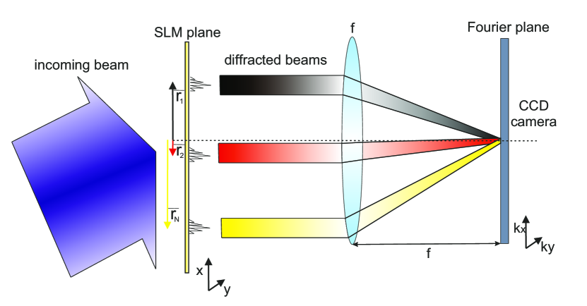
Figure 3: Concept of measurement used to retrieve the wavefront distortion. Several parallel beams diffracted off the SLM around points $\vec{r}_{i}$ are focused together and interfere on the camera placed in the Fourier plane.

IV Phase calibration

To create a map of SLM phase distortion $\phi(\vec{r})$ we measure relative phases between several parallel beams diffracted off the SLM by interfering them on a Fourier plane camera as shown in Fig. 3.

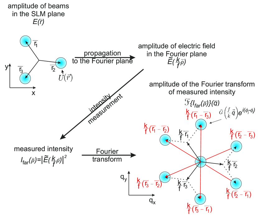
(a)

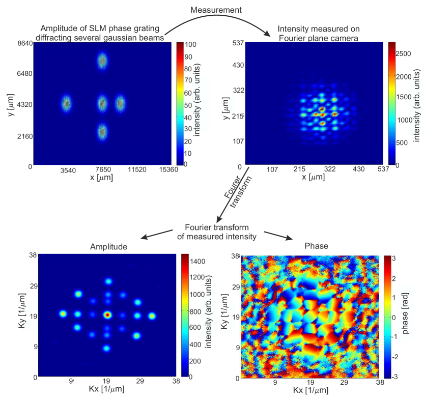
(b)

Figure 4: (a) Schematic illustration of the subsequent steps required to measure relative phases of the beams diffracted off the SLM. (b) Phase grating displayed on SLM $\Psi(x,y)$, measured intensity in the Fourier plane $I_{\text{far}}(\vec{\rho})$ and its Fourier transform $\mathcal{F}\{I_{\text{far}}(\vec{\rho})\}(\vec{q})$ (amplitude and phase).

The beams are diffracted around different points $\vec{r_{j}}=(x_{i},y_{i})$ and focus together on the far field camera. We assume all beams have same amplitude profile $U(\vec{r})$ on SLM, but may have different intensities $\alpha_{j}^{2}$ due to nonuniform illumination. The phases $\phi_{j}=\phi(\vec{r}_{j})$ of the beams are to be measured. The amplitude of the beam number $j$ in the SLM plane is therefore $\alpha_{j}U(\vec{r}-\vec{r_{j}})e^{i\phi_{j}}$. The intensity in the Fourier plane $I_{\mathrm{far}}(\vec{\rho})$ is proportional to the modulus square of the Fourier transform of the amplitude on the SLM plane. Spatial coordinates on the far field camera $\vec{\rho}$ correspond $k_{x}$ and $k_{y}$ components of the wavevectors of the Fourier decomposition of the field on the SLM through the relation $\vec{k}=k\vec{\rho}/f$ where $k=2\pi/\lambda$ is the wavevector of light and $f$ is the focal length of the Fourier transforming lens. Denoting Fourier transform of a function $f(\vec{r})$ in $\vec{k}$-space by $\mathcal{F}\{f(\vec{r})\}(\vec{k})$ we can write:

$$I_{\text{far}}(\vec{\rho}) \propto \left|\mathcal{F}\left\{\sum_{j=1}^{N}\alpha_{j}U(\vec{r}-\vec{r_{j}})e^{i\phi_{j}}\right\}\left(\frac{k}{f}\vec{\rho}\right)\right|^{2}$$ (3)

$$= \left|\sum_{j=1}^{N}\alpha_{j}\tilde{U}\left(\frac{k}{f}\vec{\rho}\right)e^{-i\frac{k}{f}\vec{\rho}\vec{r_{j}}+i\phi_{j}}\right|^{2}$$

$$= \left|\tilde{U}\left(\frac{k}{f}\vec{\rho}\right)\right|^{2}\sum_{j,l}e^{i\frac{k}{f}(\vec{r_{l}}-\vec{r_{j}})\vec{\rho}}\alpha_{j}\alpha_{l}e^{i(\phi_{j}-\phi_{l})}$$

above $N$ is the number of beams and $\tilde{U}(\vec{k})$ denotes Fourier transform of single beam amplitude profile, $\tilde{U}(\vec{k})=\mathcal{F}\{U(\vec{r})\}(\vec{k)}$. The intensity of the interference pattern is the Fourier plane $I_{\mathrm{far}}(\vec{\rho})$ is a sum of contributions from each possible pair of beams. They overlap to form a fringe modulation under the envelope set by the far field image of any single beam $\left|\tilde{U}\left({k}\vec{\rho}/f\right)\right|^{2}$.

The crucial observation is contributions to the interference pattern $I_{\text{far}}(\vec{\rho})$ coming from each pair of beams can be separated by Fourier transforming the $I_{\text{far}}(\vec{\rho})$ thus revealing the phase differences $\phi_{j}-\phi_{l}$. This step is performed numerically on a PC and transforms from the far-field coordinates $\vec{\rho}$ into its conjugate coordinates $\vec{q}$:

$$\mathcal{F}\{I_{\text{far}}(\vec{\rho})\}(\vec{q})\propto\sum_{j,l}G\left(\frac{f}{k}\Bigl{(}\vec{q}-\frac{k}{f}(\vec{r_{l}}-\vec{r_{j}})\Bigr{)}\right)\alpha_{j}\alpha_{l}e^{i(\phi_{j}-\phi_{l})}$$ (4)

where $G(\vec{q})=\mathcal{F}\left\{|\tilde{U}(\vec{k})|^{2}\right\}(\vec{q)}$ depends only on the amplitude profile $U(\vec{r})$ of each beam. The value of $G(0)$ has to be real, because it is Fourier transform of a real function. The amplitude of the Fourier transform $\mathcal{F}\{I_{\text{far}}(\vec{\rho})\}(\vec{q})$ has maxima at locations $\vec{q}_{l,j}=(\vec{r_{l}}-\vec{r_{j}})k/f$. We assume they are separated, that is each difference of the vectors $\vec{r_{l}}-\vec{r_{j}}$ is unique. Then from the formula (4) it follows that the phase at a point $\vec{q}_{l,j}=(\vec{r_{l}}-\vec{r_{j}})k/f$ equals the phase difference between respective beams $\phi_{j}-\phi_{l}$. The above steps are illustrated in Fig. 4.

Measurement with $N$ beams yields ${N(N-1)}/{2}$ phase differences, that is ${N(N-1)}/{2}$ equations for $N$ unknown phases. We find phases by least square fit.

The number of beams $N$ is limited because the vectors $\vec{r_{l}}-\vec{r}_{j}$ have to be unique. For this reason to make phase distortion map $\phi(\vec{r})$ we perform a series of measurements. We diffract $N=5$ beams, which is good tradeoff between complexity and precision. First beam is in the middle of the SLM $\vec{r}_{1}=0$ and serves as a common phase reference i.e. we take $\phi(0)=0$. Other beams are placed around central beam and shifted after acquiring each far field image so as to cover entire surface of the SLM except near the centre. To determine the phase near the centre we perform additional measurements. We choose three reference points at the periphery of the SLM and shift central beam around the middle of the SLM. By averaging all the results we retrieve the phase distortion map $\phi(\vec{r})$ presented in Fig. 5. The entire measurement consists in acquiring 700 images and takes about 5 minutes which is limited predominantly by delays in simple LabVIEW software while changing phase masks on the SLM and acquisition from the camera.

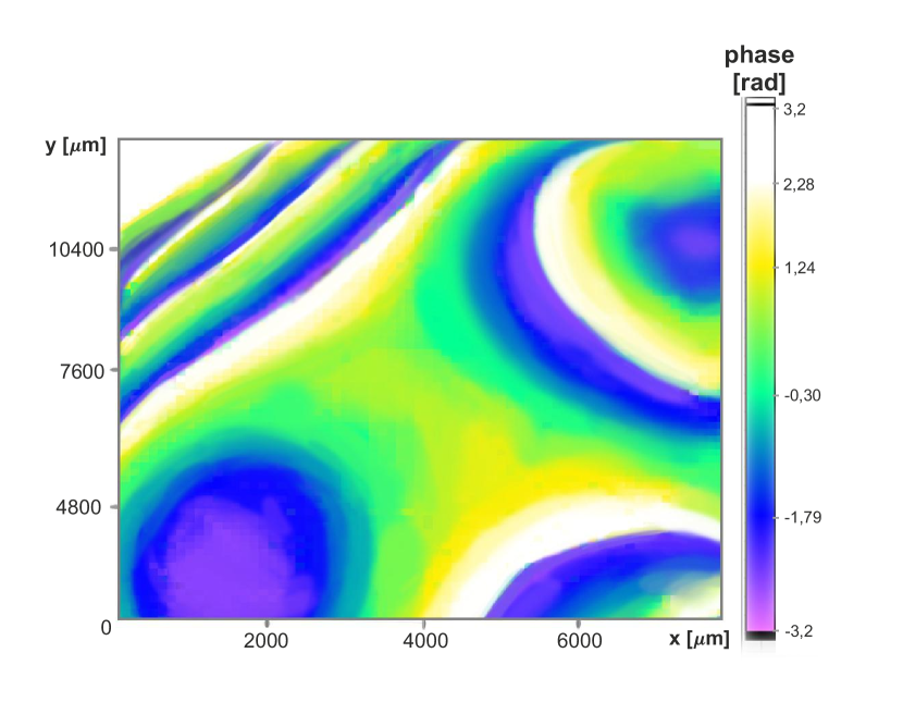
Figure 5: Phase distortion map $\phi(\vec{r})$, created by averaging results of 5-point measurements from 500 images and 4-point measurements from 200 images. This is a combined effect of the SLM, illuminating beam wavefront distortion and focusing optics.

Note the scheme of calibration described above compensates for the wavefront distortions of the optics between the SLM and a certain calibration plane which is imaged on one camera and Fourier transformed to the other camera. For proper operation of the scheme the optical setup has to fulfil the following conditions. The SLM has to be imaged with little blur, of the order of several periods of phase grating $d$ so that the desired final spatial amplitude variations at relied with sufficient fidelity. The far field camera has to register true Fourier transform of the calibration plane field. The fidelity has to be high at small angles corresponding to angular spread of probing Gaussian beams and the resolution good enough to resolve fringes due to their interference.

In our setup (depicted in Fig. 1) the calibration plane is located at the SLM image camera that is 79 mm behind the center of the PBS and the image there is magnified by a factor of $-0.7$. Due to particular lens arrangement the wavefront there is diverging with $1059$ mm radius of curvature when the entire beam is focused in the Fourier plane. Thus to produce certain wavefront $\theta(\vec{r})$ at physical location of our image plane one has to program spatial phase $\theta(\vec{r})+r^{2}/(R\lambda)$ with $R=2125$ mm due to magnification with respect to image plane.

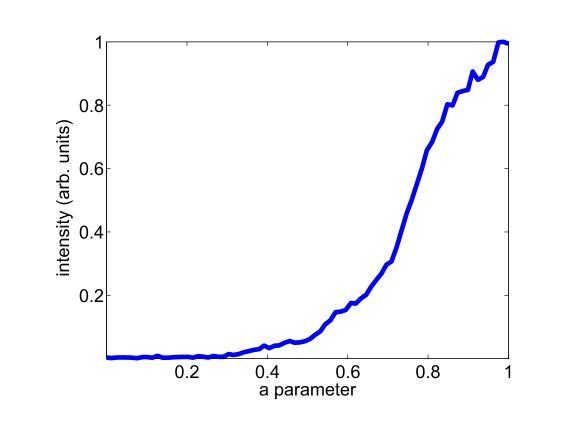
Figure 6: Measured intensity of diffracted wave $\alpha(a)^{2}$ as a function of phase grating depth $2\pi a$ normalized to unity.

V Amplitude correction

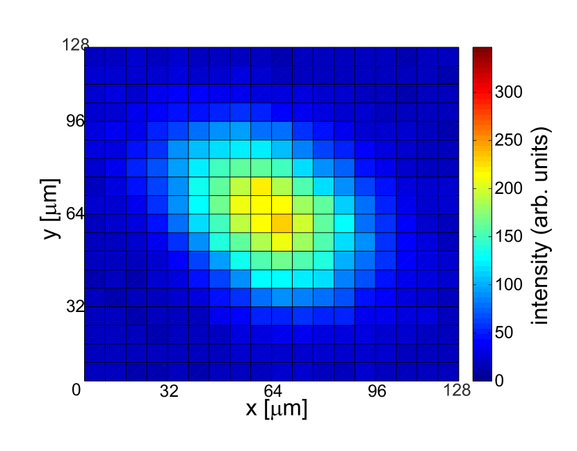
(a)

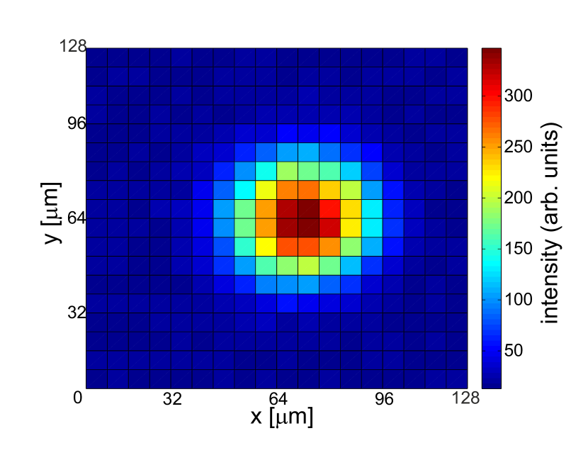
(b)

Figure 7: Intensity of Gaussian beam with 1.5 mm diameter on SLM focused on Fourier plane camera (a) before phase correction (b) after phase correction.

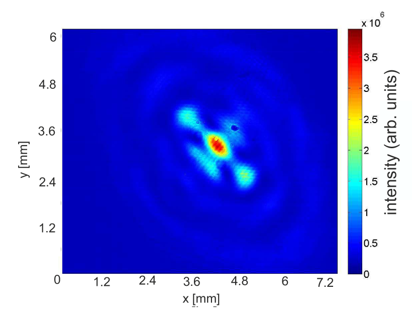
(a)

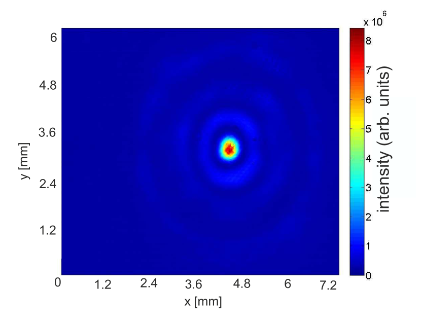
(b)

(c)

Figure 8: Intensity of zero Bessel beam diffracted off the SLM after two meters propagation (a) before phase and amplitude correction (b) after phase and amplitude correction. Figure (c) presents theoretical intensity of zero Bessel beam.

The amplitude of the beam which illuminates the SLM has certain nonuniform distribution $J(\vec{r})$. It can be measured by displaying phase grating with spatially constant depth equal $2\pi$ (see Fig. 2) on the whole SLM surface and registering an intensity distribution on image plane camera. Having measured $J(\vec{r})$ the amplitude of the beam to be diffracted can be multiplied by a factor ${\sqrt{\max\,J(\vec{r})/J(\vec{r})}}$ to compensate the effects of nonuniform illumination.

Next the diffraction efficiency versus depth of the phase grating $2\pi a$ is measured. The resulting $\alpha(a)^{2}$ normalized to unity is shown in Fig. 6. The inverse of $\alpha(a)$ function $M(\alpha)$ informs us that to diffract wave with arbitrary amplitude $\alpha$ the phase grating of depth $a=M(\alpha)$ has to be used. Correcting for nonuniform illumination the required phase grating depth at point $\vec{r}$ becomes $a=M\left[\alpha(\vec{r}){\sqrt{\max\,J(\vec{r})/J(\vec{r})}}\right]$.

VI Calibrated programming of SLM

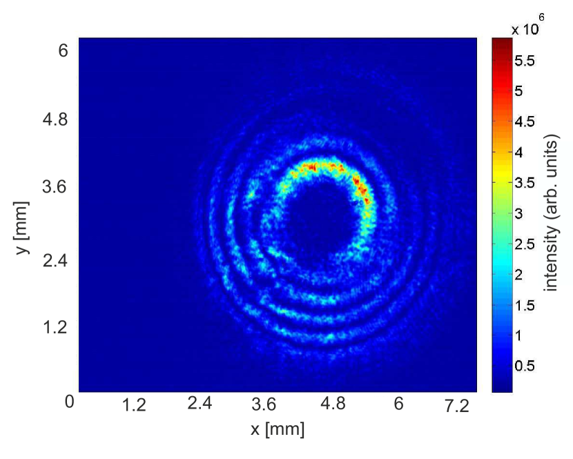
(a)

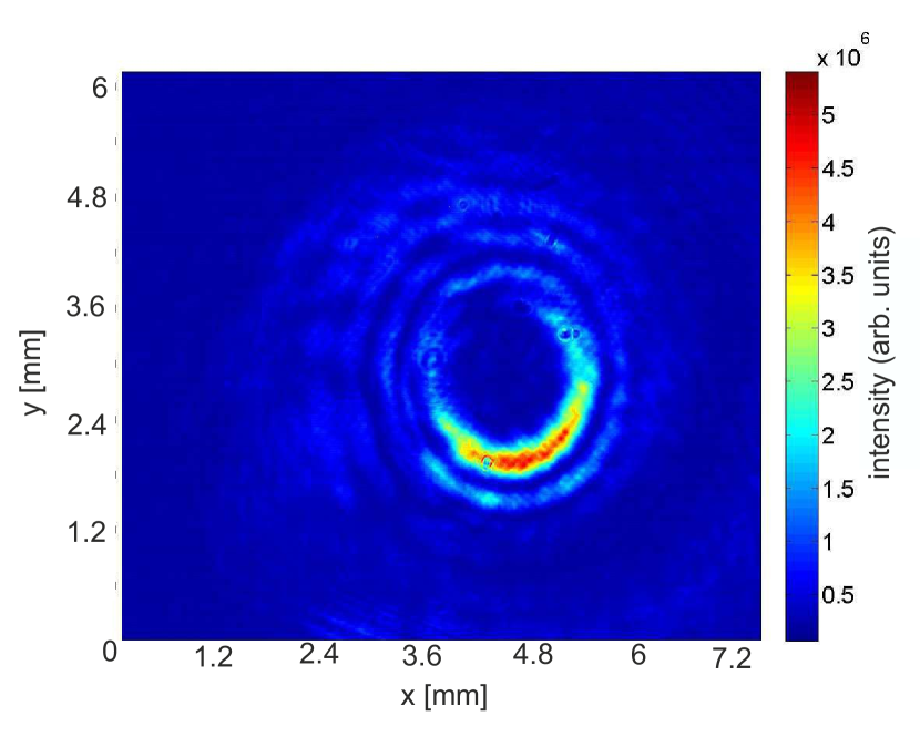
(b)

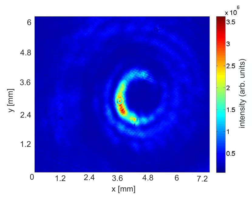
(c)

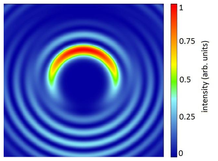
(d)

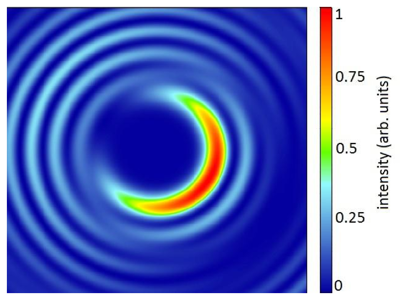
(e)

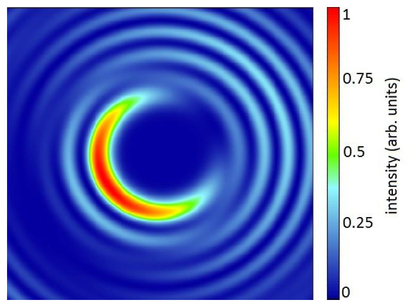
(f)

Figure 9: Intensity of seventh and eighth Bessel beam superposition (a) in the image plane of SLM and after propagation by (b) 75 cm or (c) 150 cm. Figures (d), (e) and (f) shows the simulation result.

Here we formulate a recipe for diffracting beam of any amplitude and phase profile described by function $A(\vec{r})e^{i\theta(\vec{r})}$. Suppose that $Q_{d}(\vec{r})$ is elementary grating defined in Eq. (1), $\phi(x)$ is a SLM phase distortion (see Fig. 5), ${\sqrt{\max\,J(\vec{r})/J(\vec{r})}}$ is amplitude correction factor and M($\alpha$) is inverse of diffraction efficiency function. Then to diffract the desired beam we project the following phase grating on the SLM:

$$\Psi(\vec{r}) = a(\vec{r})Q_{d}\left(x+d\frac{\theta(\vec{r})-\phi(\vec{r})}{2\pi}-\frac{d}{2}a(\vec{r}),y\right),$$ (5)

$$a(\vec{r}) = M\left(\frac{\sqrt{\max\,J(\vec{r})}}{\sqrt{J(\vec{r})}}A(\vec{r})\right).$$ (6)

The phase of grating $Q_{d}(\vec{r})$ is shifted to compensate precalibrated phase distortion $\phi(\vec{r})$ and amplitude dependent phase to produce desired wavefront $\theta(\vec{r})$ and amplitude $A(\vec{r})$.

As a first test we check Gaussian beam focusing. Gaussian beam with flat wavefront minimizes spot size in Fourier plane, so near perfect focusing confirms calibration. Fig. 7 compares measured far field intensity for a Gaussian beam diffracted off the SLM before and after calibration. Diffracted beam diameter is 1.5 mm and laser wavelength is 780 nm, so diameter of ideal Gaussian beam on the camera should be about 26 $\mu$m. We find focal plane beam diameter of 28.5 $\mu$m by fitting.

A less trivial test consists in creating Bessel beams and verifying their propagation properties. Bessel beams are solutions of wave equation which are diffraction resistant bessel . The family of Bessel beams amplitude are expressed in cylindrical coordinates by:

$$B_{n}(r,\phi,z)=J_{n}(\frac{r}{w})e^{in\phi}e^{ik_{z}z}$$ (7)

$$k_{z}=\sqrt{\frac{\omega^{2}}{c^{2}}-\frac{1}{w^{2}}}$$ (8)

where $J_{n}$ is n-order Bessel function, $w$ is the beam radius, $\frac{\omega}{2\pi}$ is frequency of light and $c$ is the speed of light.

Initially we created a 0th Bessel beam with $w=0.15\mathrm{mm}$ and verified its diffraction properties. Results are presented in Fig. 8.

Finally we created a superposition of 7th and 8th order Bessel beams. Due to different azimuthal phases the sum of these two beams looks like crescent key-1 as depicted inf Fig. 9. Moreover Eq. (8) rules that by setting different diameters $w$ of the component beams we can mismatch their phase velocities. This results in rotation of the crescent profile around beam axis along propagation. In Fig. 9 we present measured intensity of beam superposition at three distances: 0 cm, 75 cm and 150 cm from the PBS.

In addition to the tests described above we characterized the beam outgoing from our system with commercial HASO 32 Shack-Hartmann wavefront sensor. We program our modulator to diffract uniform rectangular beam. We compared the wavefronts with and without an additional lens inserted right in front of the laser (see Fig. 1) which imprinted curvature onto the wavefront illuminating the SLM. Using Shack-Hartmann sensor we retrieved an extra wavefront curvature corresponding to R=5.5 $\pm$ 0.1 m in the SLM plane, with error due to uncertanities in relay lens positions. With our method we measured R= 5.3 m. The difference between those two amounts to $\lambda/4$ wavefront difference at the rim of the SLM. The RMS deviation of raw measurements from paraboloid has random structure with RMS $\lambda/80$ in case of Shack-Hartmann sensor and RMS $\lambda/25$ in case of our method.

When the modulator is programmed to produce flat-wavefront beam in the image plane the Shack-Hartmann sensor measures $\lambda/4$ RMS deviation from flat wavefront over entire beam. To understand this result note that the path leading to the Fourier plane camera used for calibration at the path leading to Shack-Hartmann sensor differ by extra reflection from PBS and biconvex singlet lens. Thus we attribute this result to the quality of PBS stated as $\lambda/4$ by the manufacturer and spherical aberration of the lens. For experiments requiring greater wavefront precision those two elements or their equivalents have to be of better quality.

VII Conclusions

We performed proof-of-principle demonstration of a simple method to calibrate and compensate the total wavefront distortion and nonuniform illumination in an SLM setup. The method relies on diffracting several Gaussian beams off the SLM and registering their interference pattern on a camera placed in the far field. We confirmed the accuracy of calibration by diffracting the Bessel beams and a superposition of two Bessel beams which is rotating during propagation as expected. Additionally we verified our method and commercial Haso 32 Shack-Hartmann wavefront sensor.

We implemented our method using standard singlet lenses and optical components and a pair of digital cameras. The method relies on registering position of rather sparse interference fringes thus very basic cameras are sufficient. The setup could be even further simplified by performing amplitude calibration without the image plane camera. This would be accomplished by diffracting a single small beam off the SLM, scanning its position across the surface and registering the intensity using the Fourier plane camera.

Our method is well suited to compensating wavefront errors introduced by the optical elements used to rely the SLM onto the final use plane as long as this final plane is faithfully Fourier transformed onto far field camera. The algorithm presented directly probes phase differences between multiple points. Any setup sufficient for registering both near and far field properties of diffracted beams is adequate for our method. We therefore believe it could be a natural choice in a number of experiments for both diagnostic and calibration purposes.

References

- (1) D. G. Grier "A revolution in optical manipulation" Nature 424, 810-816 (2003)
- (2) E. Schonbrun, R. Piestun, P. Jordan, J. Cooper, K. D. Wulff, J. Courtial, M. Padgett, "3D interferometric optical tweezers using a single spatial light modulator", Opt. Express 13, 3777-3786 (2005)
- (3) M. Reicherter, T. Haist, E. U. Wagemann, H. J. Tiziani "Optical particle trapping with computer-generated holograms written on a liquid-crystal display", Opt. Lett. 24, 608-610 (1999)
- (4) N. Matsumoto, S. Okazaki, Y. Fukushi, H. Takamoto, T. Inoue, S. Terakawa "An adaptive approach for uniform scanning in multifocal multiphoton microscopy with a spatial light modulator" Opt. Express 22, 633-645 (2014)
- (5) S. Fürhapter, A. Jesacher, S. Bernet, M. Ritsch-Marte, "Spiral phase contrast imaging in microscopy", Opt. Express 13, 689-694 (2005)
- (6) Bo-Jui Chang, Li-Jun Chou, Yun-Ching Chang, and Su-Yu Chiang, "Isotropic image in structured illumination microscopy patterned with a spatial light modulator", Opt. Express 17, 14710-14721 (2009)
- (7) V. Boyer, R. M. Godun, G. Smirne, D. Cassettari, C. M. Chandrashekar, A. B. Deb, Z. J. Laczik, C. J. Foot, "Dynamic Manipulation of Bose-Einstein Condensates With a Spatial Light Modulator", Phys. Rev. A 73, 031402(R), (2006)
- (8) F. K. Fatemi, M. Bashkansky, and Z. Dutton, "Dynamic high-speed spatial manipulation of cold atoms using acousto-optic and spatial light modulation", Opt. Express 15, 3589-3596 (2007)
- (9) X. He, P. Xu, J. Wang, and M. Zhan, "Rotating single atoms in a ring lattice generated by a spatial light modulator", Opt Express 17, 21007-21014 (2009)
- (10) R. Dou and M. K. Giles "Phase measurement and compensation of a wave front using a twisted nematic liquid-crystal television", Appl. Optics 35, 3647-3652 (1996)
- (11) G. D. Love, "Wave-front correction and production of Zernike modes with a liquid-crystal spatial light modulator." Appl. Optiics 36, 1517-1524 (1997)
- (12) R. W. Bowman, A. J. Wright, M. J. Padgett, "An SLM-based Shack-Hartmann wavefront sensor for aberration correction in optical tweezers", J. Opt. 12 124004 (2010)
- (13) A. Jesacher, A. Schwaighofer, S. FÃŒrhapter, C. Maurer, S. Bernet, M. Ritsch-Marte "Wavefront correction of spatial light modulators using an optical vortex image", Opt. Express 15, 5801-5808 (2007)
- (14) R. W. Gerchberg, W.O Saxson "A Practical Algorithm for the Determination of Phase from Image and Diffraction Plane Pictures", Optik 35, 237246 (1972)
- (15) G. Hall, G. C. Spalding, P. J. Campagnola, J. G. White, K. W. Eliceiri "Fast localized wavefront correction using area-mapped phase-shift interferometry", Opt. Lett. 36, 2892-2894 (2011)
- (16) T. Čižmár, M. Mazilu, K. Dholakia "In situ wavefront correction and its application to micromanipulation", Nat. Photonics 4, 388 - 394 (2010)
- (17) J.A. Davis, D.M Cottrel, J.Campos, M.J. Yzuel, I. Moreno, "Encoding amplitude information onto phase-only filters", Appl. Opt. 23, 5004-5013 (1999)
- (18) J.A. Davis, D.M Cottrel, J.Campos, M.J. Yzuel, I. Moreno, "Encoding amplitude and phase information onto a binary phase only spatial light modulator", Appl. Opt. 11, 2003-2008 (2003)
- (19) J. Durnin, "Exact solutions for nondiffracting beams. I. The scalar theory", J. Opt. Soc. Am. 4, 651-654 (1987)
- (20) R. Vasilyeu, A. Dudley, N. Khilo, and A. Forbes, "Generating superpositions of higher-order Bessel beams", Opt. Express 17, 23389-23395 (2009)