Imaging Prominence Eruptions Out to 1 AU

Abstract

Views of two bright prominence eruptions trackable all the way to 1 AU are here presented, using the heliospheric imagers on the Solar TErrestrial RElations Observatory (STEREO) spacecraft. The two events first erupted from the Sun on 2011 June 7 and 2012 August 31, respectively. Only these two examples of clear prominence eruptions observable this far from the Sun could be found in the STEREO image database, emphasizing the rarity of prominence eruptions this persistently bright. For the 2011 June event, a time-dependent 3-D reconstruction of the prominence structure is made using point-by-point triangulation. This is not possible for the August event due to a poor viewing geometry. Unlike the coronal mass ejection (CME) that accompanies it, the 2011 June prominence exhibits little deceleration from the Sun to 1 AU, as a consequence moving upwards within the CME. This demonstrates that prominences are not necessarily tied to the CME’s magnetic structure far from the Sun. A mathematical framework is developed for describing the degree of self-similarity for the prominence’s expansion away from the Sun. This analysis suggests only modest deviations from self-similar expansion, but close to the Sun the prominence expands radially somewhat more rapidly than self-similarity would predict.

1 INTRODUCTION

The heliospheric imagers on the two Solar TErrestrial RElations Observatory (STEREO) spacecraft began monitoring the Sun-Earth line shortly after the launch of STEREO in 2006 October. Since then, they have demonstrated their ability to track coronal mass ejections (CMEs) from the Sun all the way to 1 AU (Harrison et al, 2008; Wood et al., 2009; Davis et al., 2009; Lugaz et al., 2012; Möstl et al., 2014). In addition to tracking CMEs, they have also provided the first images of corotating interaction regions (CIRs) moving through the inner heliosphere (Sheeley et al., 2008; Rouillard et al., 2008; Wood et al., 2010b). More rarely, prominence eruptions can also be observed in images out to 1 AU (Howard, 2015b), and this phenomenon is here studied in more detail.

Prominence eruptions are often accompanied by CMEs. Although CMEs come in a wide variety of sizes and shapes (Howard et al., 1985), the most structured and organized of them often have a three-part structure in white light coronagraph images, consisting of a bright circular rim, a dark cavity within the rim, and a bright core typically near the back of the cavity. This bright core is often interpreted as being prominence material, but CMEs with this structure are observed without accompanying prominence eruptions, so the nature of the core can be ambiguous. There are cases of erupting prominences that can be clearly tracked upwards into the fields of view of coronagraphs (e.g., Srivastava et al., 2000), in which the prominence material tends to be bright and concentrated. However, even when such cases are observed, the prominence emission often fades and becomes difficult to distinguish from the rest of the CME structure by the time it leaves the coronagraph field of view. The two events presented in this article, from 2011 June 7 and 2012 August 31, are particularly bright events which maintain their recognizable appearance in white light images from close to the Sun all the way to 1 AU.

2 OBSERVATIONS OF THE PROMINENCE ERUPTIONS

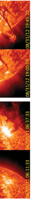
Figure 1: SDO/AIA images of the prominence eruptions from 2011 June 7 (left) and 2012 August 31 (right), showing a single pre- and post-eruption image each, for the Fe XII $\lambda$193 (top) and He II $\lambda$304 (bottom) bandpasses.

Prominence eruptions are most naturally studied near the Sun in ground-based H$\alpha$ images, or from space in the EUV. Currently, the most useful observing platform for such studies is the Atmospheric Imaging Assembly (AIA) instrument on board the Solar Dynamics Observatory (SDO). Figure 1 shows SDO/AIA images of the two prominence eruptions of interest here, from 2011 June 7 and 2012 August 31. The former was accompanied by an M2 class X-ray flare and the latter by a C8 flare. The 2011 June event is a very well studied event, being especially notable for the large amount of dark prominence material that rains back down onto the surface after the eruption (Innes et al., 2012; Williams et al., 2013; Reale et al., 2013; Gilbert et al., 2013; Carlyle et al., 2014). The 2012 August event has not garnered as much attention, but Howard (2015a, b) used it to study the relative importance of H$\alpha$ emission and Thomson scattering in white-light coronagraphic images of the erupting prominence and, unlike the studies of the 2011 June event, also followed its evolution into the inner heliosphere. Unlike the messy 2011 June eruption, the 2012 August event involves the ejection of a single, large, well-defined, loop-like filament that had been visible for weeks before finally erupting on 2012 August 31. Both of the two prominence eruptions are accompanied by bright, fast CMEs, which are trackable all the way to 1 AU along with the prominence material. The CME structures and their kinematics will be studied here along with the prominence eruptions.

This article mostly concerns observations of the prominence eruptions (and CMEs) far from the Sun, particularly with the white-light telescopes on STEREO. Each STEREO spacecraft carries four such telescopes that observe at different distances from the Sun (Howard et al., 2008). There are two coronagraphs, COR1 and COR2, that observe the Sun’s white light corona at angular distances from Sun-center of $0.37^{\circ}-1.07^{\circ}$ and $0.7^{\circ}-4.2^{\circ}$, respectively, corresponding to distances in the plane of the sky of $1.4-4.0$ R_⊙ for COR1 and $2.5-15.6$ R_⊙ for COR2. And there are two heliospheric imagers, HI1 and HI2 (Eyles et al., 2009), that monitor the interplanetary medium (IPM) in between the Sun and Earth, where HI1 observes elongation angles from Sun-center of $3.9^{\circ}-24.1^{\circ}$ and HI2 observes from $19^{\circ}-89^{\circ}$.

The two STEREO spacecraft have orbits near 1 AU, with STEREO-A leading the Earth by a steadily increasing angular distance, and STEREO-B trailing behind. Figure 2 maps the locations of Earth, STEREO-A, and STEREO-B in the ecliptic plane at the time of the two prominence eruptions. The fields of view of the HI1 and HI2 imagers are shown explicitly in the figure. Outlines of the CME structures are from 3-D reconstructions that will be described below.

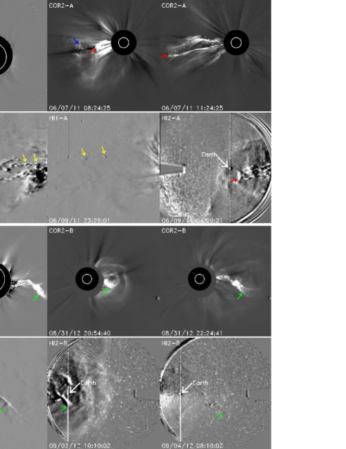
Figure 3: The top two rows are a sequence of 8 images from STEREO-A depicting the 2011 June 7 prominence eruption as it journeys from the Sun into the IPM. Similarly, the bottom two rows are a sequence of STEREO-B images showing the progression of the 2012 August 31 prominence eruption. Colored arrows identify specific parts of the prominences that can be tracked from frame to frame. Note that there are saturation artifacts in the earliest COR1 images. More comprehensive visualizations of the prominence propagation through the fields of view of the STEREO imagers are provided in two movies available in the online edition of the article.

Figure 3 displays sequences of images illustrating how STEREO can follow the two prominence eruptions far into the IPM. The COR1 and COR2 images are displayed after subtracting an average daily background. The HI1 and HI2 images are running-difference images, with the previous image subtracted from each image. For the 2011 June event, STEREO-A is best situated to track the eruption (see Figure 2), so a sequence of eight STEREO-A images is shown. For the 2012 August event, STEREO-B is the better situated platform, so eight STEREO-B images are shown. Movies of the prominence eruptions, cycling through all four of STEREO’s white-light imagers, are available in the online version of this article.

The two prominence eruptions are so bright that they actually saturate the COR1 detector, as shown in the first COR1 images of each event in Figure 3. This COR1 saturation is not common at all, so it is clear early on that these eruptions are exceptional in how bright they appear in the upper corona. The COR2 and HI1 images in Figure 3 help to place the prominence eruptions in the context of the larger CME eruptions in which they are embedded.

Colored arrows in Figure 3 are used to point to specific parts of the prominences that can be tracked from frame to frame. The most recognizable part of the 2011 June eruption is a square-topped loop. A red arrow points to the top of the southern leg of this loop. The 2012 August eruption is initially a more circular loop, as seen most clearly in the COR2-B images in Figure 3. However, the top of this loop and its northern leg quickly fade and become difficult to distinguish from the CME background structure. This is typical for prominence eruptions in white light. It is the bright southern leg of the loop that is easily trackable from COR1-B through HI2-B, and this is what the green arrow in Figure 3 is following.

The blue arrows in Figure 3 identify 2011 June prominence material ejected ahead of the aforementioned square-topped loop. This material is trackable at least into HI1 before becoming more diffuse and less recognizable as distinct from the background CME. Once again, this is the norm for prominence material. What is remarkable about the two prominence eruptions presented here are the parts of the prominence structures that remain bright, distinct, compact, and coherent all the way out to 1 AU.

The yellow arrows in Figure 3 point to two dense knots of material far down the northern leg of the square-topped loop of the 2011 June eruption. These knots actually begin to look like comets as they travel through the HI1-A field of view, with tails pointed away from the Sun. This is most easily seen in the movie of the 2011 June prominence eruption available in the online version of this article, but the tails of the “comets” are faintly visible in the third HI1-A image in Figure 3. This phenomenon indicates that these knots of material are moving more slowly than the ambient solar wind at this location. The knots are clearly dense enough that the solar wind is having difficulty picking them up and accelerating them to its speed; hence the development of the “comet tails.”

It would be nice if the extensive observations of these prominence eruptions from STEREO’s imagers could be supplemented with direct plasma measurements from in situ instruments on STEREO, or from the Wind and Advanced Composition Explorer (ACE) spacecraft operating near Earth. The images clearly show the prominence material persisting to great distances from the Sun, so the in situ signal from such an encounter should have been quite obvious and dramatic. Unfortunately, the prominence eruptions missed all of the 1 AU spacecraft, with the 2011 June 7 eruption passing in between Earth and STEREO-A and the 2012 August 31 eruption passing between Earth and STEREO-B (see Figure 2).

3 CME RECONSTRUCTION

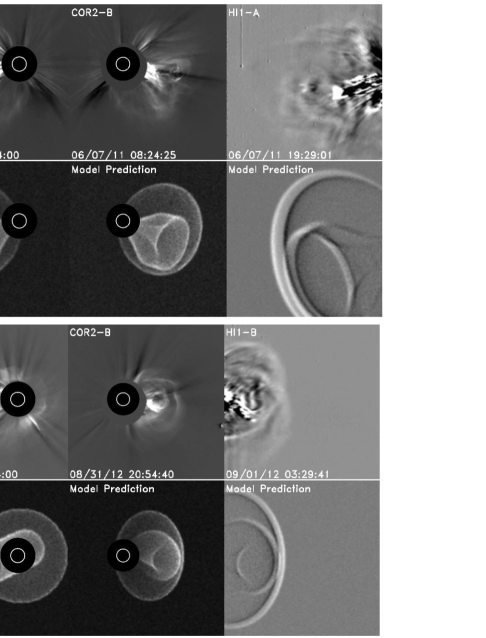
Figure 4: In the top two rows, four images of the 2011 June 7 CME are compared with the predictions of the 3-D model from Figure 5. The bottom two rows are an analogous data/model comparison for four images of the 2012 August 31 CME.

Given that the erupting prominences are incorporated into larger CME structures, a 3-D reconstruction of the two CMEs is useful to quantify the trajectory, spatial extent, and kinematics of the larger scale eruptions. Representative images of the CMEs are shown in Figure 4. These include not only images from STEREO-A and -B, but also from the C2 coronagraph on the Large Angle Spectrometric Coronagraph (LASCO) instrument on board the Solar and Heliospheric Observatory (SOHO), which operates near Earth (Brueckner et al., 1995). Observations from all three spacecraft are considered in the reconstruction analysis.

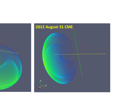
Figure 5: 3-D reconstructions of the 2011 June 7 and 2012 August 31 CME, structures in HEE coordinates, with the x-axis in red pointing towards Earth, and the z-axis in green pointing towards ecliptic north. Each model consists of a flux rope shape embedded inside a lobular shock.

The 3-D reconstructions are performed using techniques described and used extensively in past work (Wood & Howard, 2009; Wood et al., 2010a, 2011), and the reader is referred to those papers for details. In short, the CME ejecta is assumed to have the shape of a symmetric magnetic flux rope (e.g., Chen et al., 1997; Gibson & Low, 1998; Wood et al., 1999; Thernisien et al., 2009). Both of these fast CMEs have visible shock fronts out in front of the ejecta, so the 3-D shock shape is reconstructed as well, approximating it as a symmetric, lobular front. The CME structure is not assumed to vary at all with time, meaning we assume the structure expands in a self-similar fashion. There is clearly some change in structure in reality, so the trial-and-error fitting process involves compromise in deciding on a best estimate of the average CME shape from close to the Sun (in COR1 and COR2) into the IPM (in HI1 and HI2). The resulting CME structures are shown in Figure 5, each structure once again consisting of a tube-shaped magnetic flux rope embedded inside a lobular shock front. The structures are shown in heliocentric Earth ecliptic (HEE) coordinates, with the Sun at the origin, the x-axis pointed towards Earth, and the z-axis pointed towards ecliptic north. Slices through these 3-D models in the ecliptic plane are shown in Figure 2, providing another good visualization of the trajectory and spatial extent of these two CMEs. Synthetic images of the reconstructions are shown in Figure 4 for comparison with the actual images.

The reconstruction process includes a kinematic analysis of the CMEs, once again completely analogous to what has been done in past work (Wood & Howard, 2009; Wood et al., 2010a, 2011). For both events, the leading edge of the flux rope component of the CME is followed from the Sun to beyond 1 AU, with angular distance from the Sun converted to actual distance using the so-called “harmonic mean” approximation (Lugaz et al., 2009). The resulting distances are plotted versus time in the upper panels of Figure 6, for both CMEs. These distance-vs.-time measurements are fitted with a simple, multi-phase kinematic model. We have found that fast, impulsive CMEs generally have kinematic profiles that can be modeled with three phases: an constant acceleration phase very close to the Sun; a constant deceleration phase as the CME decelerates, presumably due to interaction with the slower ambient solar wind; and finally a constant velocity phase after the CME reaches its terminal velocity (Wood & Howard, 2009; Wood et al., 2011, 2012). We model our two CMEs similarly, but the 2011 June 7 CME is already at its maximum velocity early in COR1, so the first phase is omitted. The result is the fit to the data in the top panels of Figure 6, and the velocity profiles in the bottom panels. Both CMEs are quite fast, reaching speeds of 1012 km s^-1 and 1244 km s^-1, respectively. These maximum velocities are achieved very early, even before they leave the COR1 field of view. Both CMEs then decelerate significantly, mostly in the HI1 field of view.

The reconstructions suggest that the 2011 June 7 CME grazes Earth, and that the 2012 August 31 CME grazes both Earth and STEREO-B (see Figure 2). Figure 7 shows in situ plasma measurements from Wind (near Earth) during the presumed 2011 June 7 CME encounter, and from both Wind and STEREO-B during the 2012 August 31 CME encounters. Both the proton density and velocity measurements are shown, which are compared with the predicted density and velocity profiles from the 3-D reconstruction and kinematic models of the two CMEs.

For the 2012 August event, clear shocks are observed at both Wind and STEREO-B on September 3 at times when the model CME is predicted to encounter the spacecraft, providing strong support for these shocks being the 2012 August 31 event. The velocity predictions appear much too high, but comparing image and in situ velocity measurements for shocks can be tricky, because the images will be measuring the velocity of the shock, while the in situ data will be measuring the velocity of material moving through the shock. The agreement is therefore deemed good enough for our purposes. The negative slope of the predicted velocity profiles in Figure 7 is due to the self-similar expansion assumption in the 3-D reconstruction process. Evidence that the 2011 June 7 CME encounters Wind is much weaker. There is a modest density enhancement on June 10, which persists for about a day, but there is no shock or velocity increase at the beginning of the density increase. The density increase begins a few hours after the reconstruction predicts the CME shock should arrive, which is close enough to suspect that this density increase is associated with the CME.

For the 2012 August event, the existence of clear shocks at both STEREO B and Wind provides another excellent way to confront our image-based reconstruction with in situ data. By combining the in situ measurements and the Rankine-Hugoniot shock jump conditions, shock normals at STEREO-B and Wind can be inferred, which can then be compared with shock normals predicted by the shock shape in Figure 5. This is actually an ideal event for this kind of exercise, because STEREO-B and Wind are on opposite sides of the shock and should therefore see shock normals pointing in very different directions (see Figure 2).

The shock normal computation procedure is described in Wood et al. (2012), based largely on the analysis approach of Koval & Szabo (2008), who describe the methodology in even more detail. Figure 8 shows proton density, temperature, velocity, and magnetic field measurements from STEREO-B and Wind taken at the time of the shock encounter on 2012 September 3. Pre- and post-shock time periods are delineated and used to measure pre- and post-shock plasma parameters, with uncertainties estimated using the variation of the parameters within the defined 5–10 minute time range.

These pre- and post-shock plasma measurements are plugged into the Rankine-Hugoniot shock jump conditions (e.g., Lepping & Argentiero, 1971). Different shock normals can be defined by a longitude $\phi$ and latitude $\theta$ in a Sun-centered coodinate system, with the spacecraft at $(\phi,\theta)=(0^{\circ},0^{\circ})$, $\theta=90^{\circ}$ being to the north relative to the ecliptic, and $\phi=90^{\circ}$ being to the west (i.e., to the right from the spacecraft’s perspective). The goal is to determine which shock normal best meets the jump conditions, as quantified by a $\chi^{2}$ goodness-of-fit parameter. As described by Koval & Szabo (2008), the shock velocity normal to the shock in the rest frame of the shock, $V_{S}$, is generally another free parameter of the fit. However, this parameter can be eliminated using kinematic information from imaging (Wood et al., 2012). The 3-D shock reconstruction and kinematic model described above provide a measure of shock radial velocity at the spacecraft, $V_{rad}$. From Figure 7, $V_{rad}=681$ km s^-1 at STEREO-B and $V_{rad}=589$ km s^-1 at Wind. The radial velocity is related to $V_{S}$ by $V_{S}=V_{rad}\cos\phi\cos\theta$.

Figure 9 shows $\chi^{2}$ contours of the shock normal fits in the $\theta-\phi$ parameter space, and compares these measurements with the shock normals expected from the 3-D reconstruction. As expected, the shock normal is pointed to the east at STEREO-B, which is near the east edge of the shock, and the shock normal is pointed to the west at Wind, which is near the west edge of the shock (see Figure 2). The jump condition measurements of the shock normals agree very well with those predicted by the image-based shock reconstruction, with only a $21^{\circ}$ discrepancy at STEREO-B and a $33^{\circ}$ discrepancy at Wind. This result provides support for the accuracy of our 3-D CME reconstruction, and demonstrates admirable consistency between the imaging and in situ measurements of the CME.

4 PROMINENCE RECONSTRUCTION

The CME reconstruction process described in the previous section has been used in the reconstruction of a number of past events, but it does involve a number of assumptions and approximations. The analysis assumes that the CME structure is the same at all times, that it can be perfectly represented by the simple symmetric flux-rope-plus-shock paradigm, and that expansion is purely radial and self-similar. None of these assumptions are strictly true, as CME structures always have asymmetries and irregularities to their shapes that will be impossible for any parametrized representation to accurately reproduce, and CMEs often exhibit some degree of shape variation during their journey from the Sun to 1 AU. For the prominence, we utilize a 3-D reconstruction approach that does not require any a priori assumptions about the shape or time-dependence of the structure.

Specifically, the analysis approach is a point-by-point reconstruction of the time-dependent erupting prominence structure using simple triangulation from two-viewpoint STEREO images. The basic idea behind the use of two-viewpoint STEREO imagery for triangulation in 3-D reconstructions is described by Liewer et al. (2009), who focused on the 3-D reconstruction of an erupting filament close to the Sun. The technique requires simultaneous images, image A and image B, of some structure taken from two different vantage points. A point in image A marking the location of some feature corresponds to a line in 3-D space, with the feature lying somewhere along that line. The line in 3-D can be mapped onto a line in the image plane of image B. The game is then to identify where along the image B line is the structure marked in image A. Once this is known, the 3-D coordinates of the feature are known. Liewer et al. (2009) use the word “tiepointing” to describe this sort of analysis. Doing this for multiple points allows a crude mapping of the 3-D structure that is being observed.

An example is shown in Figure 10, which displays COR2-A and COR2-B images of the 2011 June event, taken at the same time. Fifteen points on the prominence structure are identified, indicating the features to be tracked as the prominence expands away from the Sun. The first ten points trace the square-topped loop that defines the most recognizable part of the structure. Point #5 basically corresponds to the red arrow in Figure 3, and points #9 and #10 correspond to the yellow arrows. Points #11-#15 identify other features that are not part of this loop, which triangulation reveals are in front of the loop from STEREO-A’s perspective. The connectivity of these last five points with each other and with the loop is unclear. In any case, point #5 in the COR2-A image in Figure 10, identifying the top of the southern leg of the loop, corresponds to the white line in the COR2-B image. This line naturally passes over the top of the southern leg of the loop in that image. Marking that location in the COR2-B image then identifies the 3-D coordinates of point #5.

The goal is to laboriously do this triangulation for all 15 points for a large set of COR1, COR2, HI1, and HI2 image pairs. There are time steps where only some of the 15 points can be properly triangulated, due to part of the prominence being out of the field of view in one or both of the STEREO images. If a given point can be marked in one of the two images, a 3-D position can be computed assuming that the trajectory direction of that feature is unchanged from the most recent time when a proper 2-point triangulation measurement is available. This approach ends up being necessary for all HI2 measurements, because while the prominence is easily visible in HI2-A (see Figure 3), it is only just barely visible in HI2-B due to the prominence simply moving too far away from STEREO-B (see Figure 2). If a given point is unavailable in either STEREO-A or STEREO-B image, a position is inferred by interpolation between 3-D positions where actual measurements are available. All this is to make sure 3-D position measurements are available for all 15 points at all considered time steps.

As a final step the distance, $r$, and direction of each point are inspected to verify that there is a reasonably smooth, self-consistent variation, where the direction is defined by a longitude, $\phi$, and a latitude, $\theta$ in HEE coordinates. To smooth point-to-point variations, and to allow for further interpolation between the sampled time steps, sixth order polynomials are fitted to plots of $\log r$ vs. time, $\phi$ vs. $\log r$, and $\theta$ vs. $\log r$. These fits, which are visually confirmed to be of excellent quality, provide the final measurements of $r$, $\phi$, and $\theta$ for all 15 points at all desired time steps.

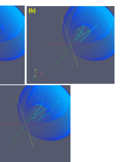
Figure 12: (a) For the 2011 June 7 eruption, the position of the evolving prominence structure is shown relative to the reconstructed CME structure, for a time corresponding to $\Delta t$=5.40 hours from a reference time of 6:30 UT on 2011 June 7. The coordinate system is HEE, with the x-axis in red pointing towards Earth, and the z-axis in green pointing towards ecliptic north. (b) Similar to (a) but for $\Delta t$=27.66 hours. (c) Similar to (a) but for $\Delta t$=56.66 hours. The top of the prominence appears to rotate slightly, and the prominence moves upwards with time relative to the CME.

The results are displayed in Figures 11 and 12. Figure 11 displays the evolving prominence structure by projecting the 3-D structure into 2-D image planes in HEE coordinates, with the first three panels of the figure focusing on the evolution of the structure close to the Sun, and the last three panels focused farther out. The first 10 points are connected with a solid line, as these represent the well-defined loop (see Figure 10). As mentioned above, the connectivity of points #11-#15 is less clear. Dotted lines are drawn between #12-#15, and point #11 is connected with #13, but whether this represents the actual magnetic field line connectivity is debatable. It is clear from Figure 11 that the material represented by points #11-#15 erupts at longitudes farther from Earth than the primary loop, which has a trajectory about $32^{\circ}$ west of Earth. For comparison, the CME flux rope of the eruption is at $40^{\circ}$ west, so the prominence loop is slightly offset from the center of the CME trajectory, but still well within its spatial extent.

This is shown explicitly in Figure 12, which shows the position of the prominence relative to the CME, based on the separate 3-D reconstructions of both. Close to the Sun, the top of the prominence is at or near the bottom of the apex of the CME flux rope, as apparent in the COR2 and HI1 images in Figures 3 and 4. The prominence seems to move upwards relative to the CME structure, suggesting that the prominence is not tightly affixed to the CME’s magnetic structure. By the time the prominence is well into the HI2-A field of view, it is clearly much closer to the leading edge of the CME front relative to distance from the Sun than is the case in COR2 and early HI1 (see Figure 3). Thus, the only way the CME and prominence could be moving in concert is if the CME structure was not expanding in a self-similar fashion. The CME reconstruction assumed self-similar expansion for the sake of simplicity, and while this is certainly an approximation it is not apparent that relaxing that approximation would dramatically improve the quality of the reconstruction.

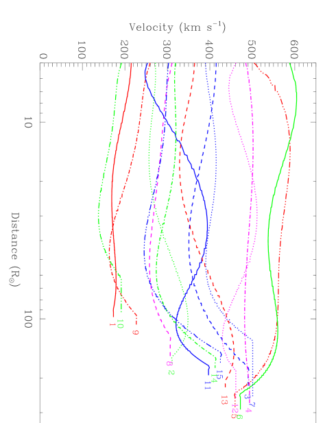
Figure 13: The speeds of the 15 points followed in the 2011 June 7 prominence (see Figure 10) are plotted versus distance from Sun-center.

This issue can be explored further kinematically. Figure 13 plots velocities measured for the 15 prominence points as a function of distance from Sun-center. The prominence points exhibit little systematic variation in velocity. (Note that the waviness of some of the velocities is an artifact of the polynomial fitting described above that smoothed out the position and direction measurements.) The top of the prominence, represented by points #5 and #6, has a speed of $500-600$ km s^-1, with at most only a very small degree of deceleration. This kinematic behavior is significantly different from that of the CME flux rope, for which there is substantial deceleration in the HI1 field of view, with the CME leading edge ultimately slowing down from its peak of 1012 km s^-1 to 468 km s^-1 early in the HI2 phase (see Figure 6). With this fundamental difference in kinematic behavior, the prominence must move upwards relative to the CME compared to what would be expected from self-similar expansion of a combined prominence-plus-CME structure. Howard (2015b) provided similar kinematic evidence for the 2012 August prominence also moving upwards relative to its CME.

Points #9 and #10 have speeds of about 200 km s^-1 near the bottom of the northern leg of the prominence loop. These are the points that start to look like comets in HI1-A (see Figure 3). Thus, the comet-like behavior is demonstrating that the ambient wind at those locations must be significantly faster than 200 km s^-1.

As far as the shape of the prominence is concerned, there are no dramatic changes in morphology as the primary loop of interest expands outwards, but the top of the loop does appear to rotate slightly at a distance of aboust 50 R_⊙. This is most apparent in Figure 11d and Figure 12. The effect is modest enough that it is within the realm of possibility that it could be due to systematic errors involved in the triangulation measurements. There are clearly uncertainties in tracking the same part of the prominence from COR1 to HI2, which could be systematic in nature, leading to systematic errors in the inferred prominence morphology.

Nevertheless, if the rotation is assumed to be real, there is an interesting way to quantify it using a quantity called “writhe,” as defined by Berger & Field (1984). This quantity has been used in the study of helicity in solar structures, both observational and theoretical (Longcope & Klapper, 1997; Linton et al., 1998; Tian et al., 2005). Writhe for the prominence loop can be defined as

$$Wr=\frac{1}{4\pi}\int_{0}^{L}\int_{0}^{L}\frac{{\bf\hat{t}}(s)\times{\bf\hat{t}}(s^{\prime})\cdot\left[{\bf X}(s)-{\bf X}(s^{\prime})\right]}{\left|{\bf X}(s)-{\bf X}(s^{\prime})\right|^{3}}ds~{}ds^{\prime},$$ (1)

where X(s) is the position vector for points along the loop, and $\hat{\bf t}$ is a tangent vector along the loop. Calculating $Wr$ requires integrating over the loop twice, and because writhe in this manner is defined over a closed loop, we have to connect the footpoints to close the prominence loop structure. The $Wr$ parameter is computed for the 2011 June 7 prominence loop, for all time steps.

Figure 14 plots $Wr$ versus distance to the top of the loop. The writhe is initially near zero while the prominence is close to the Sun, but it increases in magnitude (with a negative sign) between 30 R_⊙ and 80 R_⊙. The writhe reaches a value of $Wr\approx-0.4$. The negative magnitude indicates a lefthanded direction to the rotation. We attach no meaning to the smaller scale variations in $Wr$, such as the small bumps near 7 R_⊙ and 150 R_⊙, which are too small to be connected with any visible change in prominence structure in Figures 11 and 12. But the decrease in $Wr$ to $\sim-0.4$ clearly corresponds to the rotation of the top of the loop in Figure 11d and Figure 12. If real, the cause of this writhe is unclear. Prominence eruptions close to the Sun are often observed to be accompanied by substantial twisting and kinking, but magnetic forces will be much weaker at distances of $30-80$ R_⊙. The degree of writhe is small enough that it is possible that some independence of motion of different parts of the prominence may be enough to induce the apparent rotational motion.

Shifting focus from the 2011 June event to that of 2012 August, ideally a full reconstruction analysis would now be presented for the 2012 August eruption. Unfortunately, this is not possible. There are a couple reasons for this. One is that much of the 2012 August prominence loop seen in COR1 and COR2 becomes indistinct in HI1 and HI2, unlike the 2011 June square-topped loop, making it less attractive for analysis. But more importantly, the viewing geometry of the 2012 August event is simply not very good (see Figure 2). A point-by-point reconstruction using triangulation requires a clear association between structures seen in STEREO-A images with structures seen in STEREO-B images. This is possible for the 2011 June event, where both STEREO-A and STEREO-B essentially have lateral views of the eruption. But for the 2012 August event STEREO-B has a lateral view while STEREO-A has very much a backside view (see Figure 2). This makes it very difficult if not impossible to identify parts of the prominence in STEREO-B images with anything in the STEREO-A images.

The LASCO coronagraphs are actually more helpful for triangulation purposes, in concert with STEREO-B. Considering COR2-B and LASCO/C3 images taken as close in time as possible, a simple triangulation is made for the top of the apparent prominence when it is still fully visible, which yields an estimated longitude of $53^{\circ}$ east of Earth. This is close to the $46^{\circ}$ east longitude trajectory inferred for the center of the flux rope component of the CME (see Figure 2), and also well within the $42^{\circ}-57^{\circ}$ prominence extent quoted by Howard (2015b). Howard (2015b) have already performed a kinematic analysis of the part of the 2012 August prominence structure that is trackable to 1 AU, so kinematic measurements for this event are not presented here.

5 QUANTIFYING THE SELF-SIMILARITY OF EXPANSION

We now use our point-by-point reconstruction of the 2011 June prominence to assess the degree to which it expands in a self-similar expansion. Self-similar expansion is a common assumption for CMEs moving through the IPM, as it was for us in the CME reconstructions in Section 3. This assumption greatly simplifies that type of analysis, as it means that a structure is morphologically invariant, and all that changes with time is its size. Nevertheless, it is clear that self-similar expansion is not strictly true. Quantifying the degree of deviation from self-similarity is difficult for CMEs as a whole, because it is not easy to independently track different parts of CMEs. Unlike the prominence material that was the focus of the last section, the visible structures of CMEs tend to be broad and diffuse, making it difficult to be sure that a part of the CME seen in an image from one perspective corresponds to exactly the same part of the CME seen from a different perspective. There have nevertheless been attempts to measure velocities of different parts of CME structures in coronagraph images to assess the degree of self-similarity at early times. Low & Hundhausen (1987) report a CME velocity field very inconsistent with self-similar expansion for a fast event from 1980 September 1, but in a survey of 18 CMEs Maričić et al. (2009) find that self-similar expansion is usually a good approximation.

For the erupting 2011 June 7 prominence that was reconstructed in the last section, we can quantify the degree of self-similarity more precisely than is possible for CME structures in general. Our analysis provides 3-D velocity vectors, ${\bf V}=(v_{r},v_{\theta},v_{\phi})$, at 15 points in the prominence at all time steps. Rather than use HEE coordinates as in Figure 11, it is advantageous to rotate into a coordinate system with the x-axis pointed towards the center of the prominence, meaning the prominence is basically propagating in the x-direction. The average HEE longitude and latitude of our 15 prominence points over time are $\phi=36.5^{\circ}$ and $\theta=-2.1^{\circ}$, respectively, so that is where the x-axis is pointed. The north ecliptic pole remains in the xz-plane, meaning the new z-axis will still point in a poloidal direction, and the y-axis in an azimuthal direction.

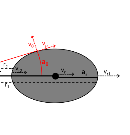
Figure 15: Schematic picture of an expanding structure at a distance $r$ from the Sun.

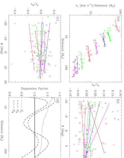
Figure 16: (a) For the 15 points followed in the 2011 June 7 prominence (see Figure 10), the radial velocity ($v_{r}$) divided by the distance is plotted versus Sun-center distance. This is done for 8 different time steps, and a linear fit is performed to each 15-point sequence. The slope of these lines is indicative of the degree of self-similarity of the expanding structure, with a slope of 0 corresponding to self-similar radial expansion. (b) For the same 8 time steps, the poloidal velocity divided by the radial velocity ($v_{\theta}/v_{\rho}$) is plotted versus poloidal angle $\theta$, and lines are again fitted to each 15-point sequence, with zero slope corresponding to self-similar expansion. Line colors and symbols are kept consistent with those used in (a). (c) Analogous to (b), but for the azimuthal velocity ($v_{\phi}$). (d) The expansion factors in the radial, azimuthal, and poloidal directions ($S_{r}$, $S_{\theta}$, and $S_{\phi}$) are plotted versus distance to the top of the prominence structure. The horizontal line corresponds to self-similar expansion.

Figure 15 provides a schematic picture of an ovoid structure expanding away from the Sun. For such a structure to maintain the same shape relative to the Sun, velocities within the structure in the direction of propagation must be proportional to distance from the Sun. Thus, in Figure 16a $v_{r}$ is divided by distance and plotted versus distance for the 15 measured points at 8 different time steps. Linear fits are performed to each sequence, with the slope of the resulting lines indicating deviation from self-similar expansion. Positive slopes are observed close to the Sun, indicating expansion greater than that expected for self-similar expansion. This slope declines with time, though, and even becomes slightly negative as the prominence approaches 1 AU.

Figure 16a provides some sense of the degree of self-similarity, but it is still desirable to assess self-similarity in a more quantitative fashion. A mathematical framework for this is now provided, with guidance provided by Figure 15. The object in the figure is shown as an oval, but our prescriptions will ultimately be independent of shape. The object is assumed to have radial and lateral extents defined by the characteristic distances $a_{r}$ and $a_{\theta}$ shown in the figure. We focus first on the case of pure radial expansion, ignoring lateral expansion for now. The front and back sides of the structure are at distances of $r_{1}=r+a_{r}$ and $r_{2}=r-a_{r}$. This object is moving away from the Sun, with the center, front, and back moving at velocities $v_{r}$, $v_{r1}$, and $v_{r2}$, respectively. If $v_{r1}\neq v_{r2}$ the structure will be changing in size, so $a_{r}=a_{r}(r)$. If it is assumed to expand (or contract) uniformly relative to its center, then $v_{r}=(v_{r1}+v_{r2})/2$. An aspect ratio for the structure is defined to be $\Lambda_{r}(r)=a_{r}(r)/r$, with differential

$$d\Lambda_{r}=\frac{1}{r}da_{r}-\frac{\Lambda_{r}}{r}dr.$$ (2)

For self-similar expansion $\Lambda_{r}$ must be constant ($d\Lambda_{r}=0$).

A useful quantification of the self-similarity of the radial expansion is

$$S_{r}\equiv\frac{1}{\Lambda_{r}}\frac{da_{r}}{dr}=\frac{r}{\Lambda_{r}}\frac{d\Lambda_{r}}{dr}+1.$$ (3)

For self-similar expansion, $S_{r}=1$. The object will be expanding faster than self-similar expansion if $S_{r}>1$, and slower if $S_{r}<1$. A value of $S_{r}=0$ corresponds to no expansion at all, and $S_{r}<0$ means the object will actually be contracting in an absolute sense as it moves away from the Sun. Since $v_{r}=dr/dt$,

$$S_{r}=\frac{1}{\Lambda_{r}v_{r}}\frac{da_{r}}{dt}.$$ (4)

From inspection of Figure 15, $da_{r}/dt=(v_{r1}-v_{r2})/2$, $v_{r}=(v_{r1}+v_{r2})/2$, $a_{r}=(r_{1}-r_{2})/2$, and $r=(r_{1}+r_{2})/2$, leading to

$$S_{r}=\frac{(r_{1}+r_{2})(v_{r1}-v_{r2})}{(r_{1}-r_{2})(v_{r1}+v_{r2})}.$$ (5)

This is the equation that will be used to quantify $S_{r}$ as a function of time and distance for the 2011 June 7 prominence.

The end points of the line segments in Figure 16a are used to provide the $r_{1}$, $v_{r1}$, $r_{2}$, and $v_{r2}$ measurements necessary to compute $S_{r}$. (This is done for all time steps, and not just the 8 shown in the figure.) Alternatively, measurements at maximum and minimum distances from the Sun could have simply been used for $r_{1}$, $v_{r1}$, $r_{2}$, and $v_{r2}$. However, the use of Figure 16a for this purpose has the advantage of allowing all 15 points to play a role in measuring $S_{r}$ at each time step, since all the points constrain the linear fits. The slopes of these lines indicate systematic deviations from self-similarity, while the scatter of the points about the lines may either indicate more random deviations from self-similarity within the structure, or may simply indicate measurement uncertainties.

In any case, the resulting $S_{r}$ measurements are shown in Figure 16d. The prominence has $S_{r}=1.3$ close to the Sun at 6 R_⊙, but this decreases to $S_{r}=1.1$ by the time the prominence is fully within the HI1 field of view. As the prominence approaches 1 AU, it decreases again, falling slightly below the self-similar value of 1 before the top reaches 1 AU, fully consistent with the slope changes seen in Figure 16a. Despite some degree of expansion different from self-similarity, the self-similar expansion approximation is actually not too bad of an approximation for this erupting prominence, with $S_{r}$ never venturing too far from unity.

A similar calculation can be used to assess expansion in the poloidal direction. Referring to Figure 15, the aspect ratio is now $\Lambda_{\theta}(\rho)=a_{\theta}(\rho)/\rho$, where for purposes of clarity in the figure $\rho$ is now being used as the radial variable instead of $r$. The expansion factor is

$$S_{\theta}\equiv\frac{1}{\Lambda_{\theta}}\frac{da_{\theta}}{d\rho}.$$ (6)

The analog of equation (4) is

$$S_{\theta}=\frac{1}{\Lambda_{\theta}v_{\rho}}\frac{da_{\theta}}{dt}.$$ (7)

It is important to note that $da_{\theta}/dt$ is affected by both $v_{\theta}$ and $v_{\rho}$, such that

$$\frac{da_{\theta}}{dt}=v_{\theta}+\Theta v_{\rho},$$ (8)

where $\Theta$ is the angular half width of the structure. Noting also that $\Theta=a_{\theta}/\rho=\Lambda_{\theta}$ (see Figure 15), this leads to

$$S_{\theta}=\frac{v_{\theta}}{\Theta v_{\rho}}+1.$$ (9)

In Figure 16b, $v_{\theta}/v_{\rho}$ is plotted versus the poloidal angle. This is done for the same 8 time steps as in Figure 16a, with linear fits once again made to each set of points. These lines should have slopes of zero in the case of self-similar expansion. The end points of the linear fits in Figure 16b provide measurements of $v_{\theta 1}/v_{\rho 1}$, $v_{\theta 2}/v_{\rho 2}$, $\theta_{1}$, and $\theta_{2}$. The angular half-width is $\Theta=(\theta_{1}-\theta_{2})/2$, which is defined relative to a center line that splits the structure into halves of equal angular width, as in Figure 15. For the upper half, we have from equation (9)

$$S_{\theta 1}=\frac{v_{\theta 1}}{\Theta v_{\rho 1}}+1.$$ (10)

For the lower half, we have

$$S_{\theta 2}=-\frac{v_{\theta 2}}{\Theta v_{\rho 2}}+1,$$ (11)

where the negative sign comes from recognizing that for the lower half of the structure a positive $v_{\theta}$ corresponds to movement towards the center line (i.e., a contraction) instead of movement away from the center line (i.e., an expansion). Our estimate of $S_{\theta}$ for the whole structure is simply the average of $S_{\theta 1}$ and $S_{\theta 2}$,

$$S_{\theta}=\frac{1}{(\theta_{1}-\theta_{2})}\left(\frac{v_{\theta 1}}{v_{\rho 1}}-\frac{v_{\theta 2}}{v_{\rho 2}}\right)+1.$$ (12)

providing the $S_{\theta}$ curve in Figure 16d. Likewise, for the azimuthal direction, an expansion factor $S_{\phi}$ can be computed,

$$S_{\phi}=\frac{1}{(\phi_{1}-\phi_{2})}\left(\frac{v_{\phi 1}}{v_{\rho 1}}-\frac{v_{\phi 2}}{v_{\rho 2}}\right)+1,$$ (13)

leading to the $S_{\phi}$ curve in Figure 16d.

As is the case for $S_{r}$, $S_{\theta}$ and $S_{\phi}$ remain relatively close to the self-similar value of 1, once again consistent with the notion that self-similar expansion is a decent approximation. Both $S_{\theta}$ and $S_{\phi}$ exhibit more variability than $S_{r}$, but it is possible that this is simply due to measurement uncertainty. Uncertainties in $S_{\theta}$ and $S_{\phi}$ will be larger than those in $S_{r}$, because while there is plenty of radial extent to the prominence, along which one can measure the radial velocity gradient, there is not much angular extent (see Figure 11), making it harder to accurately quantify the lateral velocity gradients across the width of the structure.

All three expansion factors are near 1.2 at distances of about 10 R_⊙, implying expansion somewhat greater than self-similarity while the prominence is in the COR2 field of view. The largest deviation from self-similarity is for $S_{\theta}$ far from the Sun, which plunges below $S_{\theta}=0.6$ as it approaches 1 AU. This is also indicated by the negative slopes of the lines in Figure 16b that represent the last time steps shown. This suggests expansion perpendicular to the ecliptic plane is being suppressed to some extent far from the Sun.

6 THE SCARCITY OF PROMINENCE MATERIAL AT 1 AU

The bright and compact appearance of the prominence structures in HI2 is quite distinctive from the broader, more diffuse emission generally observed in fronts of CMEs and CIRs. This means that it is possible to systematically search HI2 images for other examples of prominence material out near 1 AU. A search of the entire 2007–2014 STEREO database of HI2 images was made for this purpose. However, no other examples were found. It should be emphasized that while the database search should certainly have detected cases as bright and obvious as the 2011 June and 2012 August eruptions, it could have missed fainter examples. Nevertheless, the failure to find other clear examples of 1 AU prominence eruptions emphasizes that this is not a common phenomenon. This conclusion is consistent with in situ studies that find that it is rare to detect unambiguous cool prominence material within CMEs.

Looking within in situ CME encounters with ACE, Lepri & Zurbuchen (2010) identified regions of low charge state and low temperature with possible prominence material, finding that only 4% of CMEs encountered are observed to have such material. This makes prominence material in CMEs at 1 AU already seem rather rare, but events analogous to the two discussed in this article will be even more unusual. The 4% of cases found by Lepri & Zurbuchen (2010) are not generally accompanied by large density enhancements, including the published example, which shows only a very weak density increase. There can be no question that the 2011 June 7 and 2012 August 31 cases would have produced far more dramatic density increases than this if the prominences had encountered a spacecraft at 1 AU.

One would be hard pressed to find a published example of what an in situ encounter with the 1 AU events discussed here might look like. The 1997 January 10 event observed by Wind and discussed by Burlaga et al. (1998) may be one example. This event shows an extremely large density enhancement at the back end of a magnetic cloud ($n_{p}\approx 150$ cm^-3), with a low temperature. Burlaga et al. (1998) associate this with prominence material collected at the back of the CME flux rope, consistent with what one might expect if the 2011 June 7 prominence had been encountered by Wind. One problem with this interpretation is that the 1997 January 10 CME is followed by a CIR structure, meaning that the density enhancement may also be a pile-up associated with the CIR.

7 SUMMARY

Observations from the STEREO mission have been used to study prominence eruptions that can be tracked continuously from the Sun all the way to 1 AU. The results of this study can be summarized as follows.

1.

A full search of the HI2 image database, covering the years 2007-2014, found only two examples of clear, bright, and compact prominence emission close to 1 AU. These are eruptions from 2011 June 7 and 2012 August 31. The lack of many cases of prominence eruptions being trackable all the way to 1 AU is consistent with the rarity of cases of in situ instruments at 1 AU encountering cold, dense prominence material.

2.

Comprehensive STEREO observations of the two events and their journey through the IPM are here provided. A complete loop is apparent for both structures close to the Sun, but only for the 2011 June event can the full loop be tracked far into the IPM. For the 2011 June event, knots of material far down one leg of the loop begin to look like comets in the HI1-A field of view, as the ambient solar wind attempts to pick up and accelerate the trailing prominence material.

3.

A thorough reconstruction of the expanding prominence structure is performed for the 2011 June event, using point-by-point triangulation, allowing the morphological and kinematic evolution of the structure to be inferred from the Sun to 1 AU. Unfortunately, such an analysis is not possible for the 2012 August event due primarily to a poor viewing geometry.

4.

Comprehensive 3-D morphological and kinematic reconstructions are performed for the CMEs that accompany the two prominence eruptions, modeling the CME ejecta with flux rope shapes. Both are fast CMEs, reaching speeds greater than 1000 km s^-1, and both have visible shocks in front, the shapes of which are also modeled in the 3-D reconstructions. Both erupting prominences are directed within $10^{\circ}$ of the central trajectory of the CME flux rope.

5.

The CME reconstruction includes constraints from in situ instruments at 1 AU. The flanks of the 2012 August 31 CME shock hit STEREO-B and Wind. For the 2011 June 7 CME, Wind observes a density increase that is probably associated with a grazing incidence encounter with the CME. The CME arrival times indicated by the in situ data are well matched by the 3-D CME reconstructions for both events. For the 2012 August event, shock jump conditions provide measurements of the shock normal at STEREO-B and Wind, which agree well with the shock normals predicted by the image-based 3-D reconstruction of the shock shape.

6.

The 2011 June 7 prominence moves upwards relative to the larger CME structure enveloping it, implying that the prominence structure is not tightly affixed to the CME’s magnetic structure. The prominence kinematics are significantly different from the CME, with the CME experiencing more deceleration than any part of the prominence.

7.

The top of the 2011 June 7 prominence loop appears to rotate slightly as it moves through the HI1-A field of view, with the writhe reaching $Wr\approx-0.4$. If not due to systematic uncertainties in the reconstruction, this could be due to deformation from different parts of the loop having different nonradial velocity components rather than magnetic forces.

8.

Analysis of the expansion of the 2011 June 7 prominence structure yields a quantification of its degree of self-similarity, in both radial and lateral directions. Self-similar expansion appears to be a decent approximation for this structure, with the the expansion factors $S_{r}$, $S_{\theta}$, and $S_{\phi}$ remaining between 0.75 and 1.25 for most of the prominence’s journey to 1 AU. The radial expansion is persistently greater than self-similar until the prominence approaches 1 AU.

Figure 2: (a) Ecliptic plane map at the time of the 2011 June 7 CME and prominence eruption in heliocentric earth ecliptic coordinates, showing the positions of STEREO-A, STEREO-B, and Earth. The spatial extent of the CME in the ecliptic plane is indicated using a slice through the 3-D reconstruction described in Section 3. The dot-dashed line indicates the trajectory of the prominence eruption (see Section 4). Dotted and dashed lines indicate the fields of view of the HI1 and HI2 heliospheric imagers onboard the STEREO spacecraft, respectively. (b) Similar to (a), but for the 2012 August 31 event.

Figure 6: (a) Kinematic model of the 2011 June 7 CME based on measurements from the imagers on STEREO-A. The model follows the leading edge of the flux rope component of the CME. (b) Kinematic model of the 2012 August 31 CME based on measurements from STEREO-B, following the leading edge of its flux rope component.

Figure 7: The left panels show in situ density and velocity measurements from Wind during the time in which the 2011 June 7 CME may have encountered the spacecraft. The right panels show in situ density and velocity measurements from Wind and STEREO-B, for the time in which these spacecraft encountered the 2012 August 31 CME. The dashed lines in all panels are the density and velocity profiles predicted by the 3-D reconstructions of both CMEs described in Section 3.

Figure 8: In situ observations of the 2012 August 31 CME shock at both STEREO-B and Wind. From top to bottom the quantities are proton density, temperature, three components of velocity, and three components of magnetic field. The velocity and field components are for a spacecraft-centered RTN coordinate system with the x-axis pointing away from the Sun. Dotted lines indicate time ranges used to measure pre- and post-shock plasma parameters. These measurements and their uncertainties are shown as horizontal solid and dashed lines, respectively.

Figure 9: Shock normals relative to the Sun-observer axis, computed for the 2012 August 31 CME shock at STEREO-B (left) and Wind (right), based on the plasma measurements in Figure 8 and the Rankine-Hugoniot shock jump conditions. Diamonds indicate the best fit, with surrounding 1$\sigma$, 2$\sigma$, and 3$\sigma$ confidence intervals. Squares indicate the expected shock normal based on the image-based 3-D reconstruction in Figure 5.

Figure 10: The left panel shows a COR2-A images of the 2011 June 7 erupting prominence and marks 15 points that are tracked in STEREO imagery as the prominence expands away from the Sun. The right panel is a COR2-B image taken at the same time as the COR2-A image, with the same 15 points identified (but not labeled). The line of sight corresponding to point #5 in COR2-A, the top of the southern leg of the structure, corresponds to the white line in the COR2-B panel, which also crosses the top of the southern leg.

Figure 11: Evolution of the 2011 June 7 prominence eruption, from a 3-D reconstruction based on point-by-point triangulation, with panels (a)-(c) focusing on evolution close to the Sun and panels (d)-(f) focused further out in the IPM. The solid lines trace a loop structure seen in the eruption, based on points #1-#10 in Figure 10, while the dotted lines are based on points #11-#15 in Figure 10, with an assumed connectivity between them that is more questionable. The maps are in HEE coordinates, with the x-axis pointed towards Earth and the z-axis towards the north ecliptic pole. In panels (a)-(c) the 6 maps correspond to times of $\Delta t$=2.15, 4.33, 6.50, 8.40, 10.90, and 12.90 hours from a reference time of 6:30 UT on 2011 June 7. In panels (d)-(f), the 8 maps correspond to times of $\Delta t$=9.66, 19.65, 28.98, 38.32, 47.66, 57.66, 67.65, and 76.98 hours.

Figure 14: The writhe of the 2011 June 7 prominence loop plotted as a function of Sun-center distance to the top of the loop.

References

- Berger & Field (1984) Berger, M, A., & Field, G. B. 1984, J. Fluid Mech., 147, 133
- Brueckner et al. (1995) Brueckner, G. E, et al. 1995, Sol. Phys., 162, 357
- Burlaga et al. (1998) Burlaga, L., Fitzenreiter, R., Lepping, R., et al. 1998, J. Geophys. Res., 103, 277
- Carlyle et al. (2014) Carlyle, J., Williams, D. R., van Driel-Gesztelyi, L., et al. 2014, ApJ, 782, 87
- Chen et al. (1997) Chen, J., Howard, R. A., Brueckner, G. E., et al. 1997, ApJ, 490, L191
- Davis et al. (2009) Davis, C. J., Davies, J. A., Lockwood, M., et al. 2009, Geophys. Res. Lett., 38, L08102
- Eyles et al. (2009) Eyles, C. J., Harrison, R. A., Davis, C. J., et al. 2009, Sol. Phys., 254, 387
- Gibson & Low (1998) Gibson, S. E., & Low, B. C. 1998, ApJ, 493, 460
- Gilbert et al. (2013) Gilbert, H. R., Inglis, A. R., Mays, M. L., et al. 2013, ApJ, 776, L12
- Harrison et al (2008) Harrison, R. A., Davis, C. J., Eyles, C. J., et al. 2008, Sol. Phys., 247, 171
- Howard et al. (2008) Howard, R. A, Moses, J. D., Vourlidas, A., et al. 2008, Space Sci. Rev., 136, 67
- Howard et al. (1985) Howard, R. A., Sheeley, N. R., Jr., Michels, D. J., & Koomen, M. J. 1985, J. Geophys. Res., 90, 8173
- Howard (2015a) Howard, T. A. 2015a, ApJ, 806, 175
- Howard (2015b) Howard, T. A. 2015b, ApJ, 806, 176
- Innes et al. (2012) Innes, D. E., Cameron, R. H., Fletcher, L., Inhester, B., & Solanki, S. K. 2012, A&A, 540, L10
- Koval & Szabo (2008) Koval, A., & Szabo, A. 2008, J. Geophys. Res., 113, A10110
- Lepping & Argentiero (1971) Lepping, R. P., & Argentiero, P. D. 1971, J. Geophys. Res., 76, 4349
- Lepri & Zurbuchen (2010) Lepri, S. T., & Zurbuchen, T. H. 2010, ApJ, 723, L22
- Liewer et al. (2009) Liewer, P. C., de Jong, E. M., Hall, J. R., et al. 2009, Sol. Phys., 256, 57
- Linton et al. (1998) Linton, M. G., Dahlburg, R. B., Fisher, G. H., & Longcope, D. W. 1998, ApJ, 507, 404
- Longcope & Klapper (1997) Longcope, D. W., & Klapper, I. 1997, 488, 443
- Low & Hundhausen (1987) Low, B. C., & Hundhausen, A. J. 1987, J. Geophys. Res., 92, 2221
- Lugaz et al. (2012) Lugaz, N., Kintner, P., Möstl, C., et al. 2012, Sol. Phys., 279, 497
- Lugaz et al. (2009) Lugaz, N., Vourlidas, A., & Roussev, I. I. 2009, Ann. Geophys., 27, 3479
- Maričić et al. (2009) Maričić, D., Vršnak, B., & Roša, D. 2009, Sol. Phys., 260, 177
- Möstl et al. (2014) Möstl, C., Amla, K., Hall, J. R., et al. 2014, ApJ, 787, 119
- Reale et al. (2013) Reale, F., Orlando, S., Testa, P., et al. 2013, Science, 341, 251
- Rouillard et al. (2008) Rouillard, A. P., Davies, J. A., Forsyth, R. J., et al. 2008, Geophys. Res. Lett., 35, L10110
- Sheeley et al. (2008) Sheeley, N. R., Jr., Herbst, A. D., Palatchi, C. A., et al. 2008, ApJ, 675, 853
- Srivastava et al. (2000) Srivastava, N., Schwenn, R., Inhester, B., Martin, S. F., & Hanaoka, Y. 2000, ApJ, 534, 468
- Thernisien et al. (2009) Thernisien, A., Vourlidas, A., & Howard, R. A. 2009, Sol. Phys., 256, 111
- Tian et al. (2005) Tian, L, Alexander, D., Liu, Y., & Yang, J. 2005, Sol. Phys., 229, 63
- Williams et al. (2013) Williams, D. R., Baker, D., & van Driel-Gesztelyi, L. 2013, ApJ, 764, 165
- Wood & Howard (2009) Wood, B. E., & Howard, R. A. 2009, ApJ, 702, 901
- Wood et al. (2009) Wood, B. E., Howard, R. A., Plunkett, S. P., & Socker, D. G. 2009, ApJ, 694, 707
- Wood et al. (2010a) Wood, B. E., Howard, R. A., & Socker, D. G. 2010a, ApJ, 715, 1524
- Wood et al. (2010b) Wood, B. E., Howard, R. A., Thernisien, A., & Socker, D. G. 2010b, ApJ, 708, L89
- Wood et al. (1999) Wood, B. E., Karovska, M., Chen, J., et al. 1999, ApJ, 512, 484
- Wood et al. (2011) Wood, B. E., Wu, C. -C., Howard, R. A., Socker, D. G., & Rouillard, A. P. 2011, ApJ, 729, 70
- Wood et al. (2012) Wood, B. E., Wu, C. -C., Rouillard, A. P., Howard, R. A., & Socker, D. G. 2012, ApJ, 755, 43