Tunneling in energy eigenstates and complex quantum trajectories

Abstract

Complex quantum trajectory approach, which arose from a modified de Broglie-Bohm interpretation of quantum mechanics, has attracted much attention in recent years. The exact complex trajectories for the Eckart potential barrier and the soft potential step, plotted in a previous work, show that more trajectories link the left and right regions of the barrier, when the energy is increased. In this paper, we evaluate the reflection probability using a new ansatz based on these observations, as the ratio between the total probabilities of reflected and incident trajectories. While doing this, we also put to test the complex-extended probability density previously postulated for these quantum trajectories. The new ansatz is preferred since the evaluation is solely done with the help of the complex-extended probability density along the imaginary direction and the trajectory pattern itself. The calculations are performed for a rectangular potential barrier, symmetric Eckart and Morse barriers, and a soft potential step. The predictions are in perfect agreement with the standard results for potentials such as the rectangular potential barrier. For the other potentials, there is very good agreement with standard results, but it is exact only for low and high energies. For moderate energies, there are slight deviations. These deviations result from the periodicity of the trajectory pattern along the imaginary axis and have a maximum value only as much as $0.1\%$ of the standard value. Measurement of such deviation shall provide an opportunity to falsify the ansatz.

1 Introduction

A modified de Broglie-Bohm (MdBB) approach to quantum mechanics was proposed in 2001 mvj1 and the complex quantum trajectories envisaged in it were drawn for several cases. This approach used the Schrodinger equation rewritten into a ‘quantum Hamilton-Jacobi equation’ qhj_eqn1 ; qhj_eqn2 ; qhj_eqn3 ; qhj_eqn4 and employed an equation of motion, both of which are similar to those used in the well-known de Broglie-Bohm (dBB) formalism db1 ; valentini ; bohm ; holland . But the MdBB quantum trajectories contain all the information in the wave function and are laid out in a complex space (with $x\equiv x_{r}+ix_{i}$ in one-dimension) and the scheme offers a different interpretation of quantum mechanics sanz_comment ; goldfarb_reply ; sanz_review than the dBB theory. For the reason that the equation of motion used here is not based on Jacobi’s theorem, just as the dBB scheme, this too cannot be termed a ‘quantum Hamilton-Jacobi formalism’. (A candidate for a ‘quantum Hamilton-Jacobi formalism’, which uses Jacobi’s theorem, is the Floyd-Faraggi-Matone (FFM) real trajectory representation floyd ; faraggi ; carroll .) The MdBB complex trajectory formalism could solve the problem of zero particle velocity for real wave function encountered in the dBB approach and was found capable of explaining many other quantum behaviour in a natural way yang1 ; yang2 ; sanz_local . Earlier, the dBB approach has helped to develop a computational method called quantum trajectory method (QTM) wyatt99 to synthesize the Schrodinger wave function on the real axis. In recent years, also the MdBB approach has been developed as a computational tool for this purpose sanz_review . Bohmian mechanics with complex action goldfarb method is aimed at obtaining the wave function directly from the complex trajectories, as in QTM, and was found more accurate. With the same spirit and by the same time, an alternative synthetic approach using complex trajectories was developed by Chou and Wyatt wyatt1 ; wyatt2 , with applications in both bound states and scattering systems.

A clear advantage of the MdBB complex representation over other trajectory formalisms is that in it the Born probability distribution along the real line can be directly obtained from the velocity field mvj_prob1 . It is seen that an exponential function involving the integral of the imaginary part of the MdBB velocity field provides this distribution in such a way that on the real line, the more we are inside the closed trajectories, the larger is the probability density. No other trajectory representation provides such an interpretation. Another feature special to the complex trajectory approach is an extended probability density in the complex plane. This issue was first addressed by Poirier poirier , who proposed a complexified analytic probability density defined by $\Psi^{\star}(x^{\star})\Psi(x)$, the product of the wave function and its generalized complex conjugate, and showed that it satisfies a complexified flux continuity equation in the complex plane. An alternative probability density of the form $\rho(x_{r},x_{i})$ in the complex space, which obeys a continuity equation and which agrees with the Born probability along the real line in most regions of the complex plane was proposed in mvj_prob1 . This expression involves an integral of the imaginary part of the sum of kinetic and potential energies along the trajectories and is also obtained by direct solving of an appropriate continuity equation. A problem with this scheme is that in some regions of the complex plane, the distribution does not agree with Born’s probability along the real line. Chou and Wyatt wyatt_prob1 have pointed out that the density proposed by Poirier mentioned above does not match the node structure of the wave function. In place of it, they have proposed an extended Born probability density $\Psi^{\star}(x)\Psi(x)$ in the complex space wyatt_prob1 . The authors could derive the Eulerian rate equation for this density wyatt_prob2 , though as pointed out by them, this distribution does not obey a complex version continuity equation due to its nonanalyticity. Later, it was observed that in the regions left out in Ref. mvj_prob1 , a trajectory integral of the above type (which involves only the kinetic energy in place of the sum of kinetic and potential energies), can agree with the Born probability density mvj_prob2 . This latter density was identified to be the same as the complex-extended $\Psi^{\star}(x)\Psi(x)$ proposed earlier wyatt_prob1 . However, we note that in regions where the potential $V=0$, the two extended probability densities are described by identical expressions.

In this paper, we put to test the complex-extended probability distribution described above wyatt_prob1 ; wyatt_prob2 ; mvj_prob2 . This is by using it and the trajectory pattern to explain the quantum phenomenon of tunneling in energy eigenstates. Tunneling of particles in eigenstates is an interesting problem in itself and is well-studied in standard quantum mechanics flugge ; zafar . But in the literature on dBB quantum theory, we are unable to find any demonstration of tunneling in energy eigenstates. It appears that in this scheme, for such eigenstates, all trajectories which approach the barrier get transmitted norsen . The FFM trajectory representation describes in the incident region the creation and annihilation of pairs of trajectories going in opposite directions floyd_tunnel , thus bringing in pair production in a nonrelativistic theory. On the other hand, in the complex MdBB method, the trajectory pattern in the complex plane, as plotted for a rectangular potential step mvj1 , shows clearly how certain trajectories in the incident region correspond to particles moving towards the barrier and get transmitted, whereas some others correspond to particles reflected back from it. For realistic, smooth potentials such as the symmetric Eckart potential and the soft potential step, the complex trajectory patterns drawn for eigenstates by Chou and Wyatt wyatt_eckart ; wyatt_eckart1 explicitly show this behaviour. But we note that the transmission and reflection probabilities are so far evaluated only for wave packets goldfarb ; wyatt1 ; rowland . The procedure adopted in those cases is to start with a wave packet impinging on the potential barrier and then to evaluate the Born probability on the other side of the barrier, along the real line, after a sufficiently long time. In their work, the complex quantum trajectory method is used as just a computational tool as in the dBB case, since only the probability distribution on the real line plays any role in it. In the present attempt, we assume the extended probability density wyatt_prob1 ; mvj_prob2 for energy eigenstates and then, using the complex trajectory pattern, compute the probabilities corresponding to the trajectories which actually tunnel or get reflected from the barrier.

In Sec. II, we shall state our ansatz and evaluate the reflection probability for a rectangular potential barrier. In Sec. III, a continuous potential barrier, with the Eckart and Morse barriers as special cases is considered for this purpose. In Sec. IV, reflection probability for a soft potential step is evaluated. The probabilities we obtain using the new ansatz are exact for the rectangular potentials. For continuous potentials, they are in excellent agreement with the corresponding results in standard quantum mechanics for low and high energies, but slight deviations are noted for moderate energies. The last section comprises a discussion of these results and our conclusions.

2 Tunneling a Rectangular Potential Barrier

In the simplest one-dimensional version of tunneling, we have the superposition of an incoming and a reflected wave on one side of a square potential barrier ($V=V_{0}$, for $|x|<a$ and $V=0$, for $|x|>a$), given by

$$\psi(x)=Ae^{ikx}+Be^{-ikx},$$ (1)

where $k=\sqrt{2mE}/\hbar$. Inside the barrier, the solution is of the form

$$\psi(x)=Ce^{-\kappa x}+De^{+\kappa x}.$$ (2)

Here $\kappa=\sqrt{2m(V_{0}-E)}/\hbar$. Assuming the particle to be incident from left ($x<-a$), we have only

$$\psi(x)=Fe^{ikx},$$ (3)

as the wave function on the right side ($x>a$). In the standard case, we evaluate the tunneling probability as $T(k)\equiv|F|^{2}/|A|^{2}$ and the reflection probability as $R(k)\equiv|B|^{2}/|A|^{2}$. The matching conditions, namely, the continuity of the wave function and its space derivative on the boundaries at $x=\pm a$, help to evaluate the tunneling probability as

$$T(k)=\frac{1}{1+[1+(\epsilon^{2}/4)]\sinh^{2}(2\kappa a)},$$ (4)

where $\epsilon=(\kappa/k)-(k/\kappa)$. The above wave functions $\psi(x)$ constitute an energy eigenstate of the particle, with a fixed value for its energy. Since this is a time-independent problem with definite energy, we have $\Delta E=0$ and it is meaningless to use the uncertainty relation $\Delta E\Delta t\geq\hbar$ to explain tunneling. As mentioned above, a more general description of tunneling phenomenon in standard quantum mechanics involves a wave packet impinging on such a barrier. For evaluating the tunneling probability in this case, one evaluates the total probability on the other side of the barrier, a long time after the packet reaches it. But we may note that also in this approach, there is a long-standing debate over whether it leads to superluminal speeds for the particles as the width of the barrier exceeds certain value, a predicted phenomenon which is referred to as Hartmann effect hartman . In the case of a square potential barrier, even for an energy eigenstate, the tunneling time is given by an expression that approaches a constant for thick barriers, implying an issue concerning superluminal propagation, even though physical causality is not violated davies . Hence it is desirable to look forward to alternative formalisms, such as quantum trajectory representations, for more insight on quantum tunneling in energy eigenstates.

First we consider the dBB formalism. This scheme adopts the standard Born probability axiom so that the trajectories do not have any particular role in the evaluation of reflection and transmission probabilities. It is easy to see that in the incident region where $\psi$ is given by Eq. (1), the velocity of particles given by de Broglie’s equation of motion,

$$\dot{x}=\frac{\hbar}{2im}\frac{\left(\psi^{\star}\frac{\partial\psi}{\partial x}-\frac{\partial\psi^{\star}}{\partial x}\psi\right)}{\psi^{\star}\psi},$$ (5)

is always positive, assuming $|A|>|B|$. Thus according to this theory, in this region, we have particles traveling only towards the barrier. This means that the dBB scheme disagrees with standard quantum mechanics in the tunneling of particles in energy eigenstates. Thus, in this scheme, by accepting Born’s probability rule as an axiom at the outset, the discrepancy is swept under the rug. Continuing with the use the standard probability axiom without relating probability to the trajectories gives the wrong impression that dBB agrees with standard quantum mechanics in the prediction of tunneling in eigenstates.

On the other hand, the MdBB approach helps to predict the tunneling probability on the basis of the properties of the trajectories itself and using the expression for the complex-extended probability density. The velocity field given by the MdBB equation of motion is

$$\dot{x}=\frac{\hbar}{im}\frac{1}{\psi}\frac{\partial\psi}{\partial x},$$ (6)

which is defined in the complex plane. Integrating this, we get the complex quantum trajectories. For a rectangular potential barrier, the trajectories are as shown in Fig. 1. The matching conditions on $\psi$ at the points $x=-a$ and $x=+a$ ($a$ is real), with which the coefficients $A$, $B$, etc. in equations (1)-(3) are evaluated, can be understood as the conditions for the continuity of the MdBB velocity field (6) at these points. At other points along these boundaries at $x_{r}=\pm a$, for the rectangular potential barrier, the velocity field may not be continuous, though the trajectories can remain continuous. Another special feature to be noted is that there are trajectories emanating from some points along these boundaries (such as those points at $x_{r}=+a$, for $x_{i}>\delta$ shown in figure). These trajectories move in opposite directions and proceed either to the left or right sides. (Existence of such points, which may be called repellers wyatt_eckart ; wyatt_eckart1 , is a general feature of complex trajectories in scattering problems. In the following, we too demonstrate this in specific examples of realistic potentials.)

Next, let us consider a ‘pole’ for $\dot{x}$ (where $\psi=0$) in the complex plane, on the incident side wyatt1 . Let this point be denoted as $\alpha+i\beta$. One can see that along a line $x_{r}=\alpha$ parallel to the imaginary axis, $\dot{x}_{r}>0$ when $x_{i}<\beta$ and $\dot{x}_{r}<0$ for $x_{i}>\beta$. Thus when the equation of motion is integrated, in the $x_{r}<-a$ region, we obtain trajectories of incident particles crossing this line towards the barrier, for $x_{i}<\beta$. Similarly, trajectories for reflected particles cross this line in the reverse direction, for $x_{i}>\beta$. On the other ($x_{r}>a$) side of the barrier, we have only the transmitted trajectories for all values of $x_{i}$. It is seen that some of these trajectories emanate from points (which are repellers) on the boundary line $x_{r}=a$, with $x_{i}>\delta$, as shown in Fig. 1. The various types of trajectories obtained, for an energy $E=0.98$, are drawn with different colors. In this paper, we show that the existence of such intuitively clear trajectory picture helps to evaluate the reflection and transmission probabilities.

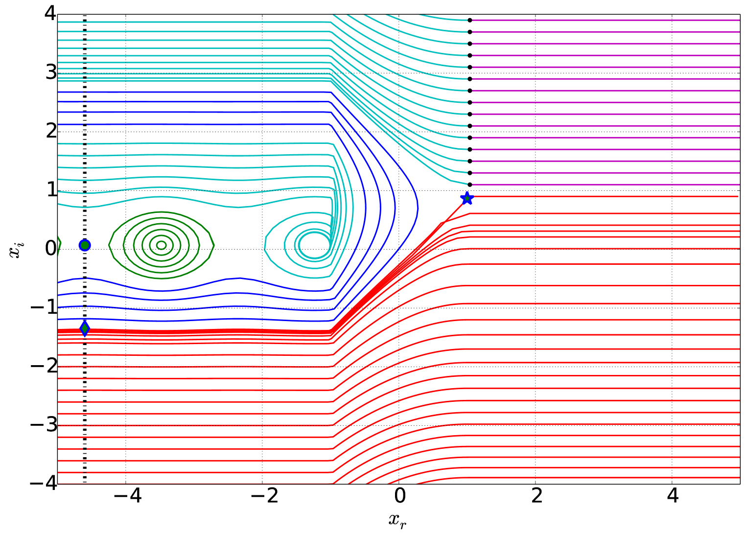
Figure 1: MdBB complex quantum trajectories for a rectangular potential barrier. The three regions, whose common boundaries are at $x_{r}=-1$ and $x_{r}=+1$, have their characteristic trajectories obtained by integrating the equation of motion (6) using the respective wave functions (1)-(3). These trajectories are drawn for an energy E=0.98. Color codes are as follows: Trajectories incident from bottom left and which tunnel through the barrier (red), similar trajectories which are reflected back (blue), closed loops (green), trajectories emanating from repellers and moving towards either left or right (cyan or magenta, in the respective order). The points $\alpha+i\beta=-4.5998+0.0681\;i$, $\gamma=-4.5998-1.347\;i$ and $\delta=1+0.865\;i$ are marked with blue symbols $\bullet$, $\diamond$, and $\star$, respectively.

In the original paper of MdBB formulation mvj1 , it was proposed that the probability axiom apply in the same manner as that in the dBB approach; i.e., by obeying Born’s probability density on the real line. As stated above, this density is generalized to the complex-extended probability density mvj_prob1 ; wyatt_prob1 ; mvj_prob2 . The present work attempts to show that one can evaluate the tunneling and reflection probabilities by making direct use of the extended probability density, together with a new definition of reflection probability based on the properties of the trajectories. This new definition involves the ratio of two integrals, both of which are evaluated along the above-mentioned line $x_{r}=\alpha$ ($\alpha$ real and negative), passing through a pole for $\dot{x}$ (where $\psi=0$) and parallel to the imaginary axis. The integrand in both cases is the extended probability density $\psi^{\star}(x)\psi(x)$. The integral in the numerator gives the total probability of reflected trajectories, obtained by integrating $\psi^{\star}(x)\psi(x)$ over them (i.e., for the part of the line with $x_{i}>\beta$) and the integral in the denominator is the total probability of incident trajectories, obtained by integrating this density over all such trajectories (i.e., for $x_{i}<\beta$). In the present case of the rectangular potential barrier, the $\psi^{\star}\psi$ probability density diverges as $x_{i}\rightarrow\pm\infty$. Hence, we must take the integrals from $x_{i}=\beta$ to $+\Lambda$ and from $x_{i}=-\Lambda$ to $\beta$, respectively, and then take the limit $\Lambda\rightarrow\infty$. It is seen that the value converges in the limit. Thus the new ansatz for the reflection probability is

$$R(k)=\lim_{\Lambda\to\infty}\frac{\int_{\beta}^{\Lambda}\psi^{\star}\psi\;dx_{i}}{\int_{-\Lambda}^{\beta}\psi^{\star}\psi\;dx_{i}}.$$ (7)

The reflection probability evaluated numerically using this ansatz is shown in Fig. 2, which is in good agreement with standard result $R(k)=1-T(k)$, where $T(k)$ is given by Eq. (4). When $\Lambda$ is finite, there are some deviations for moderate energies ($E\approx V_{0}$), but we notice that such deviations disappear for $\Lambda\rightarrow\infty$.

Though we have evaluated the above expression numerically, it is easy to see analytically, by substituting (1) in (7), that $R(k)\rightarrow|B|^{2}/|A|^{2}$ in the limit $\Lambda\rightarrow\infty$. The line of integration is parallel to the imaginary axis and passes through a pole of the velocity field so that it avoids the separatrix surrounding the web of nodes. For energy $E\rightarrow 0$, the value of $\beta$ is close to zero and the trajectory pattern is symmetric about the real line. So the above ratio tends to the value unity, equal to that in the standard calculation. For energies $E>0$ too, the ratio tends to the value $|B|^{2}/|A|^{2}$ since the integrals are not sensitive to the relatively small values of $\beta$ wyatt1 when compared to large values of $\Lambda$ as $\Lambda\rightarrow\infty$.

The primary motivation for choosing the expression (7) as the reflection probability is that it is the ratio between the probability for the reflected trajectories and that for the incident trajectories, evaluated along the line $x_{r}=\alpha$ on the incident side of the complex plane. The fact that it is able to reproduce the exact values obtained in standard calculations encourages us to use a similar expression for reflection probability, also in the case of realistic potentials. This is discussed in the next sections.

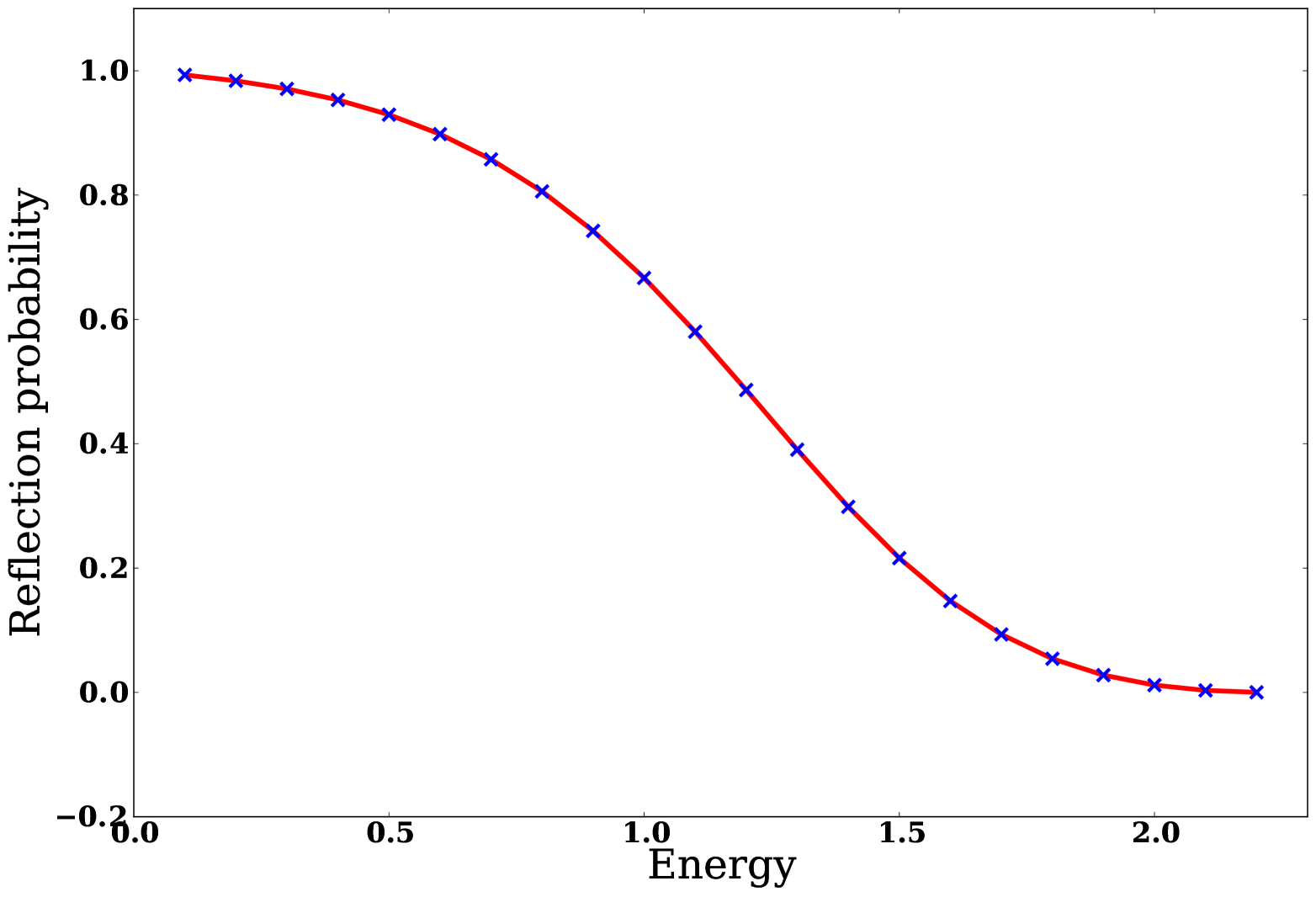
Figure 2: Reflection probability for a rectangular potential barrier, for the energy values $0.1\leq E\leq 2.2$. Blue x marks indicate values obtained using ansatz (7) and red continuous line indicates values obtained in standard quantum mechanics.

3 Tunneling the Eckart and Morse Barriers

We may note that the rectangular potential barrier is just an idealization. Therefore it is desirable to look into the case of more realistic potentials, such as the symmetric Eckart and Morse potential barriers or the soft potential step. Before that, let us consider an arbitrary potential barrier whose peak along the real axis is at $x=0$. At large distances from the barrier ($x_{r}\rightarrow\pm\infty$), let the potential be such that $V\rightarrow 0$. The time-independent Schrodinger equation has asymptotic solutions of the form found in Eqs. (1) and (3). (But it may be noted that in the MdBB approach, we have their analytic continuations, with $x=x_{r}+ix_{i}$, as solutions.) In the following, we consider a class of such potentials, which exhibit periodicity along the imaginary line. With the corresponding period denoted as $2L$, we modify our ansatz for reflection probability as

$$R(k)=\frac{\int_{\beta}^{L}\psi^{\star}\psi\;dx_{i}}{\int_{-L}^{\beta}\psi^{\star}\psi\;dx_{i}}.$$ (8)

The value of $x_{r}=\alpha$ (on the line along which the integrals are taken) must be sufficiently large and negative. Note that here also, the numerator and the denominator represent the total probability for the reflected and incident trajectories, respectively.

The Eckart and Morse barriers are special cases of a potential barrier in one-dimension studied by Ahmed zafar , of the form

$$V(x)=V_{0}\left\{1-\left[\frac{1-\exp(x/a)}{1+c\exp(x/a)}\right]^{2}\right\}.$$ (9)

When $c=0$, it is the Morse barrier and when $c=1$, this gives the symmetric Eckart barrier. Using the transformation $z=-c\exp(x/a)$, and using $b^{2}=1/c^{2}$, $\Delta=\hbar^{2}/(2ma^{2})$, $f^{2}=E/\Delta$, $q^{2}=V_{0}/\Delta$, and

$$s=\sqrt{f^{2}+(b^{2}-1)q^{2}},$$

$$g=\sqrt{q^{2}(b+1)^{2}-(1/4)},$$

$$k=\sqrt{2mE}/\hbar,$$

and

$$k^{\prime}=\sqrt{2m[E+(b^{2}-1)V_{0}]}/\hbar,$$

the exact solutions for the Schrodinger equation are obtained zafar , in terms of the hypergeometric functions. One such solution is

$$\psi_{i}=(-1)^{-if}(2f)^{-1/2}\exp(-\pi f)z^{if}(1-z)^{(1/2)-ig}{}_{2}F_{1}[(\frac{1}{2}+if-ig-is),$$

$$(\frac{1}{2}+if-ig+is),(1+2if);z]\exp(-iEt/\hbar),$$ (10)

which behaves as $\exp[i(kx-Et/\hbar))]$ as $x\rightarrow-\infty$, denoting a wave function $\psi_{i}$ incident on the barrier. Changing $k$ to $-k$ in this gives another solution

$$\psi_{\rho}=(-1)^{if}(2f)^{-1/2}\exp(\pi f)z^{-if}(1-z)^{(1/2)-ig}{}_{2}F_{1}[(\frac{1}{2}-if-ig-is),$$

$$(\frac{1}{2}-if-ig+is),(1-2if);z]\exp(-iEt/\hbar).$$ (11)

This represents an oppositely traveling, reflected wave. Another useful solution is

$$\psi_{\tau}=(-1)^{if}(2s)^{-1/2}\exp(-\pi f)z^{-if}(1-z)^{is+if}{}_{2}F_{1}[(\frac{1}{2}-if-ig-is),$$

$$(\frac{1}{2}-if+ig-is),(1-2is);(1-z)^{-1}]\exp(-iEt/\hbar),$$ (12)

which in the limit $x\rightarrow+\infty$ denotes a wave $\exp[i(k^{\prime}x-Et/\hbar)]$ being transmitted through the barrier. Assuming a desirable relation among $\psi_{i}$, $\psi_{\rho}$, and $\psi_{\tau}$ zafar , namely,

$$\psi_{i}+\rho(k)\psi_{\rho}=\tau(k)\psi_{\tau},$$ (13)

one can evaluate the reflection and transmission amplitudes $\rho(k)$ and $\tau(k)$, respectively. The corresponding probabilities are found as $R(k)=\rho^{*}(k)\rho(k)$ and $T(k)=\tau^{*}(k)\tau(k)$. Explicitly, we get

$$R(k)=\frac{\cosh[\pi(f+g-s)]\cosh[\pi(f-g-s)]}{\cosh([\pi(f+s+g)]\cosh[\pi(f+s-g)]},$$ (14)

and

$$T(k)=\frac{\sinh(2\pi f)\sinh(2\pi s)}{\cosh([\pi(f+s+g)]\cosh[\pi(f+s-g)]}.$$ (15)

We note that the derivation of these expressions for $R(k)$ and $T(k)$ depends on the assumption (13). But as can be seen from wyatt_eckart ; wyatt_eckart1 , the MdBB trajectory pattern is obtained with $\psi_{\tau}$ alone and this formalism clearly distinguishes incoming, reflected and transmitted trajectories. In the present paper, we show that also the above probabilities are obtainable from $\psi_{\tau}$ alone, with the help of ansatz (8).

The analytic continuations into the complex plane of the Eckart, Morse and other potentials discussed below in this paper have periodicity along the imaginary axis. Since they contain a factor $\exp(x/a)$, these potentials given by Ahmed’s expression (9) have the same value for $x=x_{r}+ix_{i}$ and $x=x_{r}+i(x_{i}+2\pi a)$. Furthermore, the complex powers are calculated using the principal values of the argument of the complex number $x$ by specifying $-\pi<\arg(x)\leq+\pi$, and this gives rise to a discontinuity of the velocity field along $x_{i}=\pm\pi ai$, $\pm 3\pi ai$, … for $x_{r}<0$. The trajectory pattern so obtained has the same periodicity as that of the potentials. This is explicitly shown further below, while plotting trajectories in specific cases.

, ,

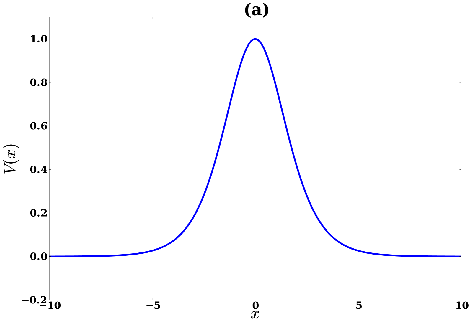
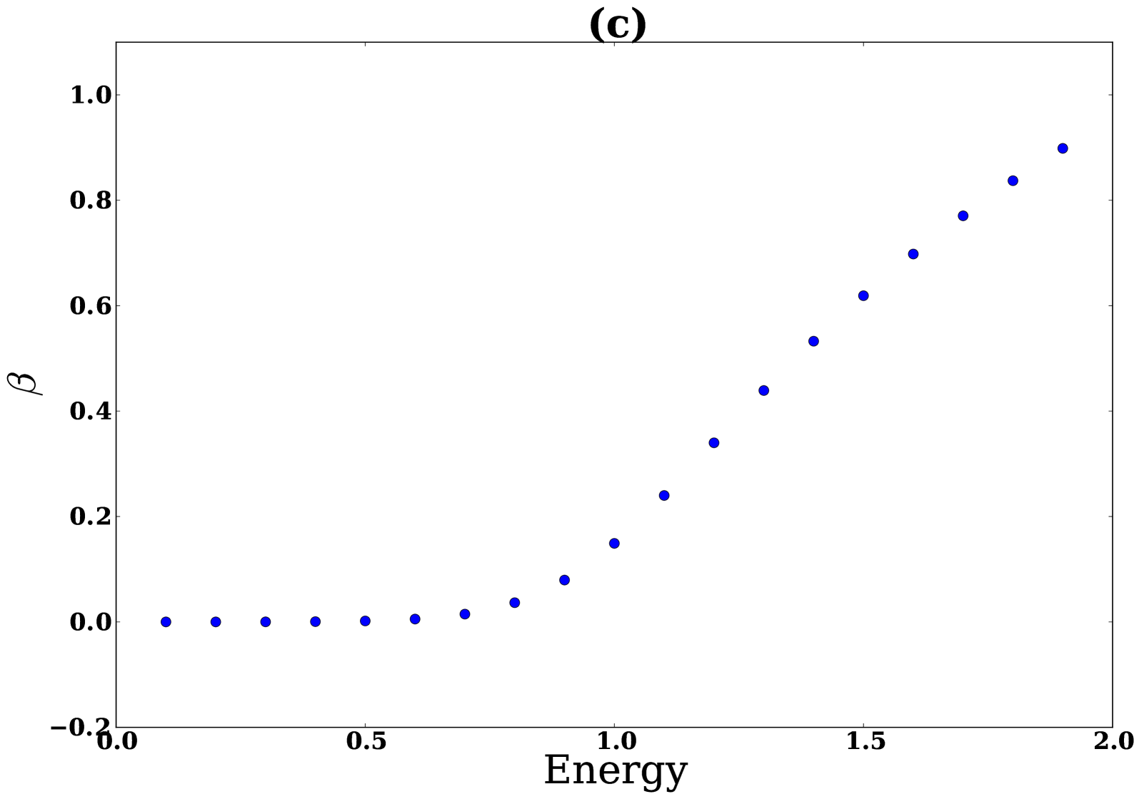
Figure 3: (a) Symmetric Eckart potential (b) Variation of the parameter $\gamma$ with energy for symmetric Eckart potential (c) Variation of the parameter $\beta$ with energy for symmetric Eckart potential

We choose the symmetric Eckart potential case [Fig. 3(a)] by putting $c=1$ in the above equations and plot the complex trajectories using $\psi_{\tau}$ in the equation of motion (6). This is repeated for various energies $E$. We fix $V_{0}=1$, $a=1$ and $\Delta=\hbar^{2}/(2ma^{2})=1/2$. The trajectory pattern for various energies drawn in Fig. 4 are the same as those obtained earlier by Chou and Wyatt wyatt_eckart ; wyatt_eckart1 . There is a periodicity in the pattern along the imaginary direction, with period $2\pi$ and hence we need only to consider the interval [$-\pi$,$\pi$] in this case. It may be noted that when $E\ll V_{0}$, very few trajectories tunnel and all the rest get reflected. But as the energy increases, more and more trajectories tunnel. As in the previous section, let us consider a line $x_{r}=\alpha$, which is parallel to the imaginary axis and which passes through a pole for the velocity field (where $\psi=0$) at $\alpha+i\beta$. Here $\alpha$ must be large and negative. We denote the value of $x_{i}$, corresponding to the top-most tunneling trajectory (among the incident trajectories) when it crosses this line, as $\gamma$. As in the rectangular potential barrier case, the top-most incident trajectory while crossing this line hits the pole for the velocity field, where $x_{i}=\beta$. Here, it must be noted that the values of $\alpha$, $\beta$ and $\gamma$ vary with energy. Graphs showing the variation of $\gamma$ and $\beta$ with energy are given in Figs. 3(b) and 3(c), respectively.

, ,
,

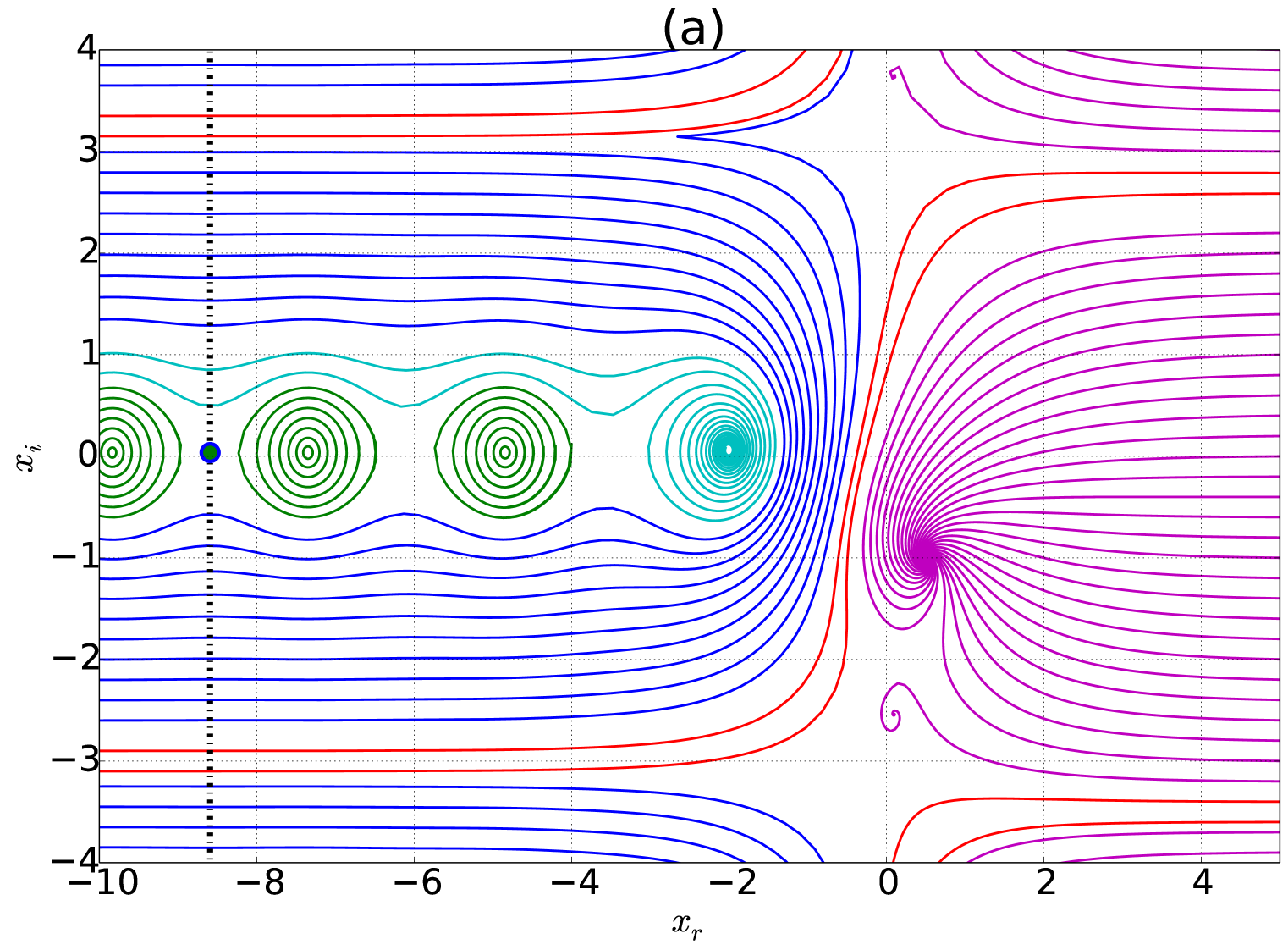
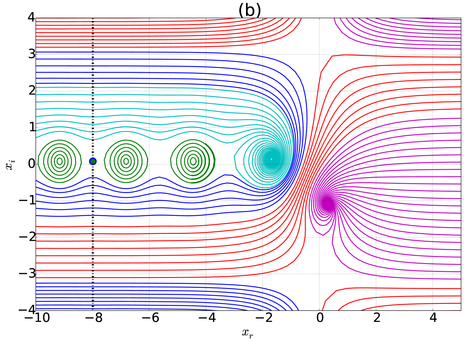
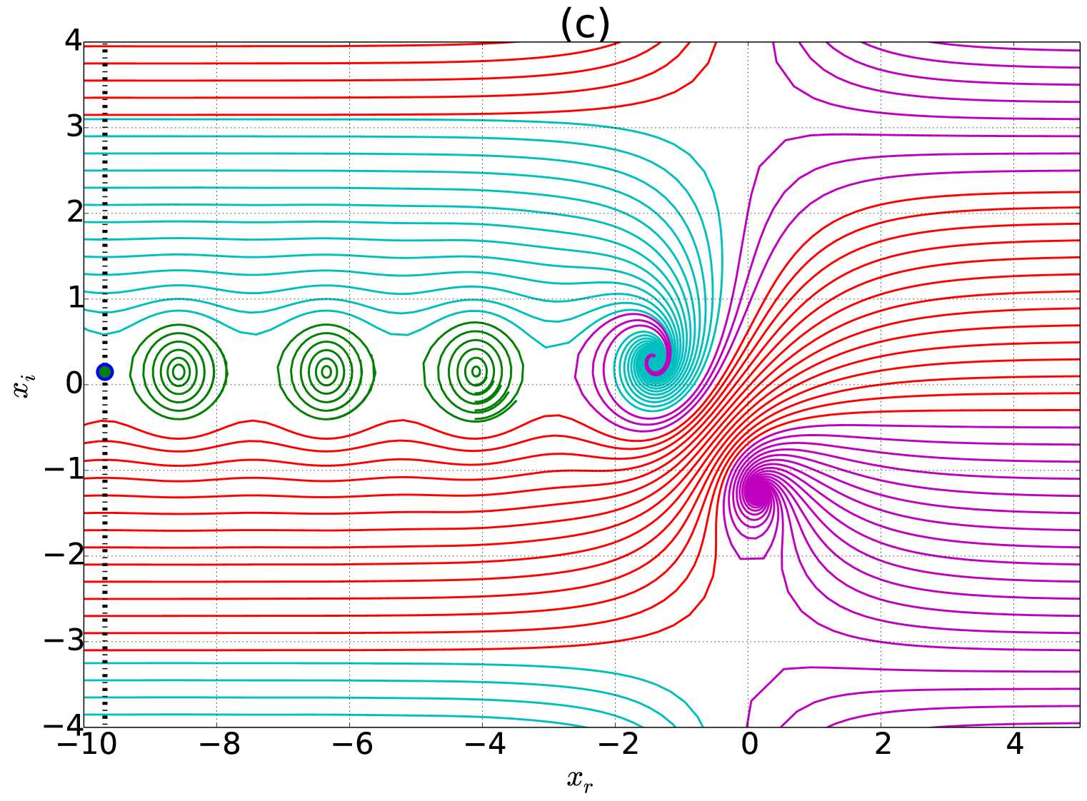
Figure 4: Complex quantum trajectories for symmetric Eckart potential, for the energy values (a) $E=0.8$, (b) $E=0.9$ (c) $E=1.0$ and (d) $E=1.2$. Color codes are as in Fig. 1. In each panel, the points $\alpha+i\beta$, whose numerical values are $-8.5918+0.036484\;i$, $-7.98707+0.079476\;i$, $-9.68208+0.149013\;i$, $-8.65166+0.339926\;i$, respectively, are marked with $\bullet$ symbols.

Using the ansatz (8) to evaluate the reflection probability for the symmetric Eckart potential, with the period $2L=2\pi$, we observe that there is very good agreement with the standard result (14). The two graphs for the range $0.1<E<2$ are plotted together in Fig. 5(a). However, slight deviations from standard result for moderate energies, with the peak of the deviation reaching $0.9\times 10^{-3}$ at $E=0.95$, is observed. [See Fig. 5(b).] This deviation is due to the periodicity of the pattern along the imaginary direction. The periodicity, with constant period, is there for all $x_{r}$ and hence we cannot attribute the deviations to the choice of $\alpha$. Since the ansatz (8) has the special feature of being independent of the assumption (13) and is based on the characteristic properties of the trajectory pattern, we hold that the present results deserve further investigations. See that the maximum value of the deviation in this case amounts to only of the order of $0.1\%$ of the actual value. If the deviations are within the measurable range, this prediction provides an opportunity to falsify the ansatz.

,

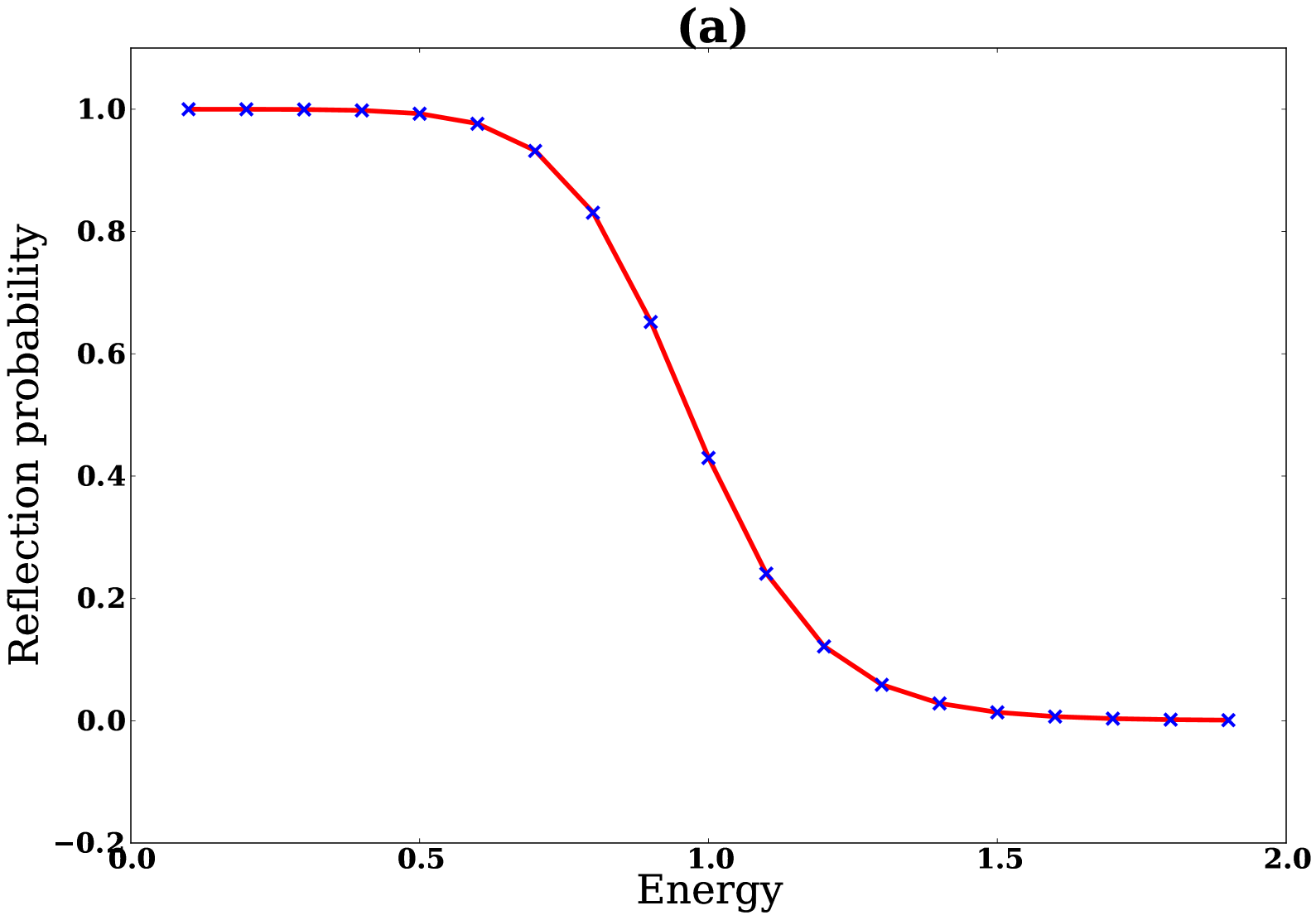
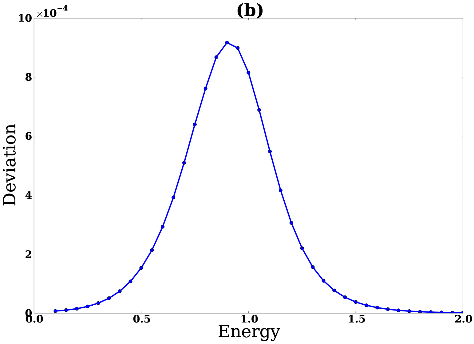
Figure 5: (a) Reflection probability for symmetric Eckart potential with peak value $V_{0}=1$, for the energy values $0.1<E<2$. Blue x marks indicates values obtained using ansatz (8) and red continuous line indicate values obtained in standard quantum mechanics (b) Deviation of reflection probability with standard values, for the energy interval $0.1\leq E\leq 2$ of a symmetric Eckart potential (with peak value $V_{0}=1$).

Similar results for a potential close to the Morse potential barrier [with $c=0.001$ in Ahmed’s potential (9) and depicted in Fig. 6(a)] are obtained. The reflection probability versus energy, while using the MdBB approach, is plotted along with the standard results in Fig. 6(b). These are again found to be in very good agreement. As in the case of the Eckart potential, there are very small deviations for reflection probability in the case of moderate energies. Deviation of reflection probability from standard values for this potential is given in Fig. 6(c).

, ,

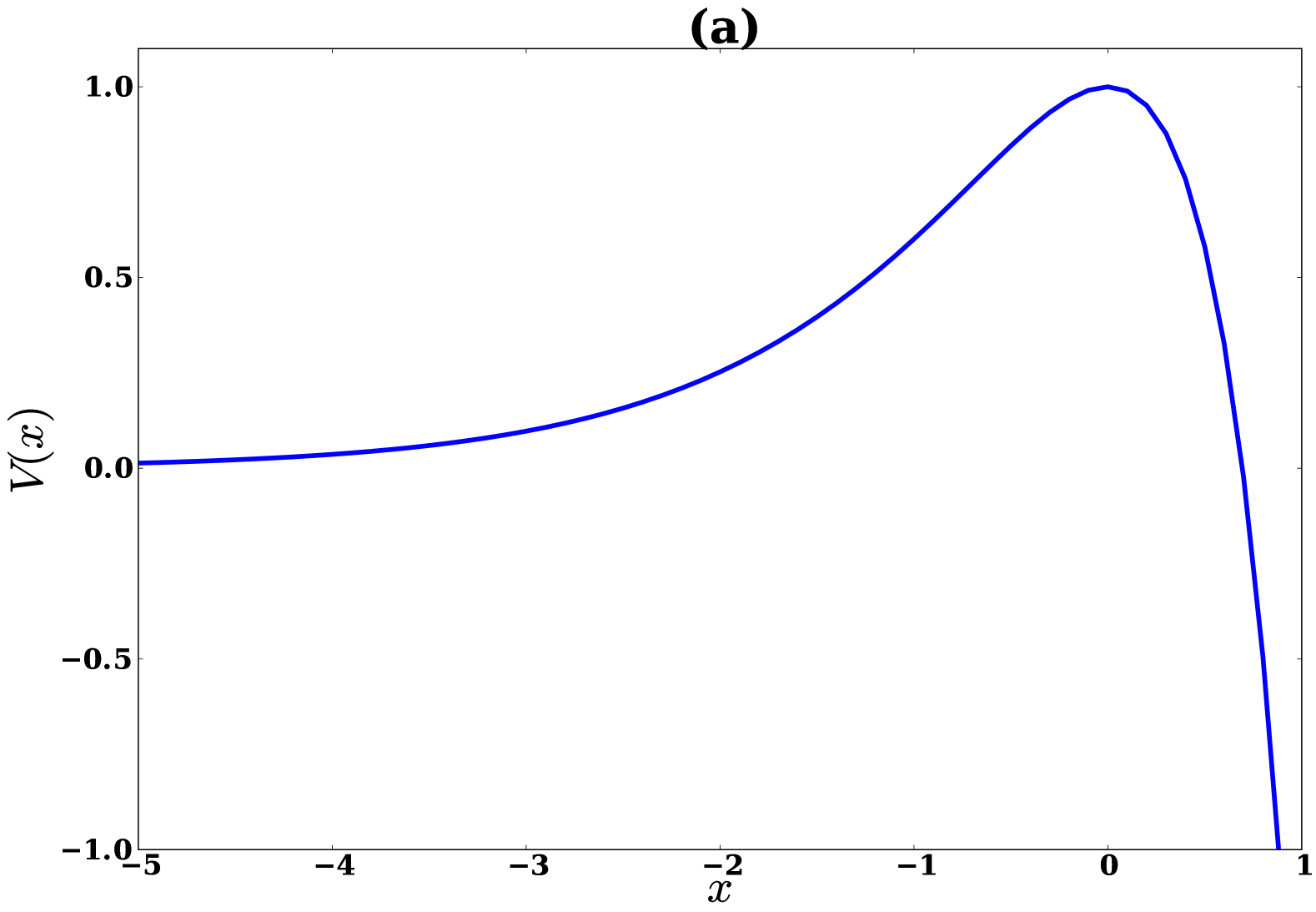
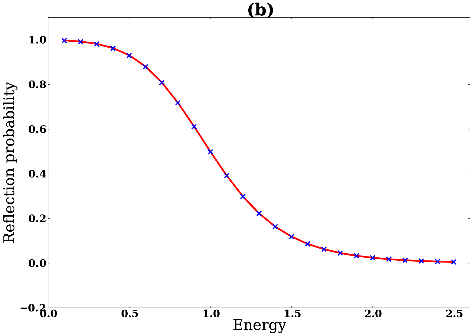
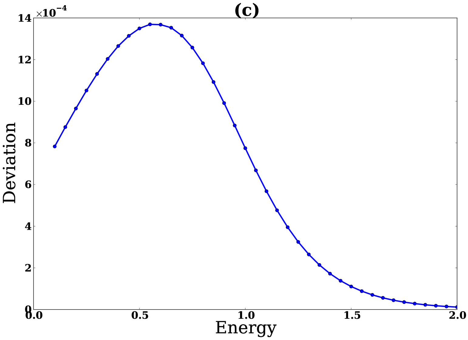
Figure 6: (a) A potential very close to the Morse potential barrier (b) Reflection probability for the above potential close to the Morse barrier, with peak value $V_{0}=1$. Blue x marks indicate values obtained using ansatz (8) and red continuous line indicates values obtained in standard quantum mechanics (c) Deviation of reflection probability with standard values, for the above potential close to the Morse barrier.

Another potential midway between the Eckart and the Morse barriers [with $c=0.5$ in Ahmed’s potential (9) and depicted in Fig. 7(a)] also shows excellent agreement with standard results, for low and high energies, as can be seen from Fig. 7(b).

,

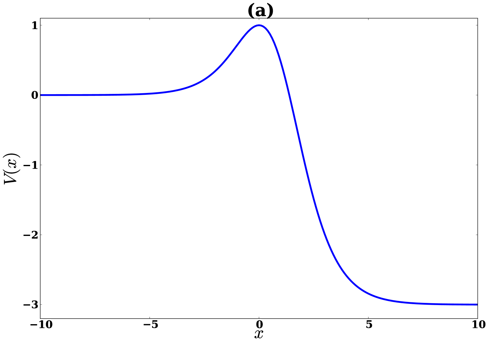
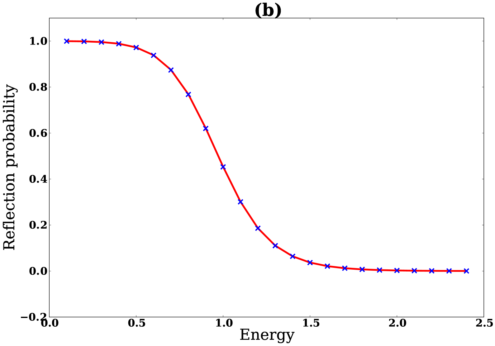
Figure 7: (a) One-dimensional potential barrier (9) with $c=0.5$ (b) Reflection probability for the potential barrier (9), with $c=0.5$ and peak value $V_{0}=1$. Blue x marks indicate values obtained using ansatz (8) and red continuous line indicates values obtained in standard quantum mechanics.

4 Transmission Over the Soft Potential Step

The complex quantum trajectories for a rectangular potential step mvj1 show no periodicity. Hence for evaluating the reflection probability in this case, one needs to use the ansatz (7). We have seen that when this is worked out, there is perfect agreement with standard result, as $\Lambda\rightarrow\infty$. In this section, we turn to the evaluation of the probability for a soft potential step, which shows periodicity along the imaginary axis. Thus we consider a soft potential step of the form flugge ,

$$V(x)=\frac{1}{2}V_{0}\left(1+\tanh\frac{x}{2a}\right).$$ (16)

The potential $V\rightarrow 0$ as $x\rightarrow-\infty$ and $V\rightarrow V_{0}$ as $x\rightarrow\infty$, as shown in Fig. 8(a). Since they contain a factor $\exp(x/a)$, also these potentials have periodicity along the imaginary direction, as in the case of Ahmed’s potential discussed above. Using $y=(1+e^{x/a})^{-1}$ instead of the variable $x$, the solution to the time-independent Schrodinger equation can be written in the form flugge

$$u(y)=y^{\nu}(1-y)^{\mu}f(y).$$ (17)

Here

$$\nu^{2}=\frac{2ma^{2}}{\hbar^{2}}(V_{0}-E),\qquad\mu^{2}=-\frac{2ma^{2}}{\hbar^{2}}E,$$

and $f(y)$ is given by

$$f(y)=C\;{}_{2}F_{1}(\mu+\nu,\mu+\nu+1,2\nu+1;y),$$ (18)

where the constant $C$ is to be fixed to satisfy the boundary conditions. However, the present MdBB approach does not need the value of $C$ to evaluate the reflection probability. Instead, with the value of $x_{i}=\beta$ corresponding to a pole for $\dot{x}$ as described above, we can evaluate $R(k)$ by using the ansatz (8). Complex trajectories for the soft potential step, for values of energies $E=0.98V_{0}$, $E=1.0V_{0}$, and $E=1.02V_{0}$, respectively, are plotted in Fig. 9. Here also, the trajectory pattern shows periodicity along the imaginary axis, with period $2L=2\pi$.

,

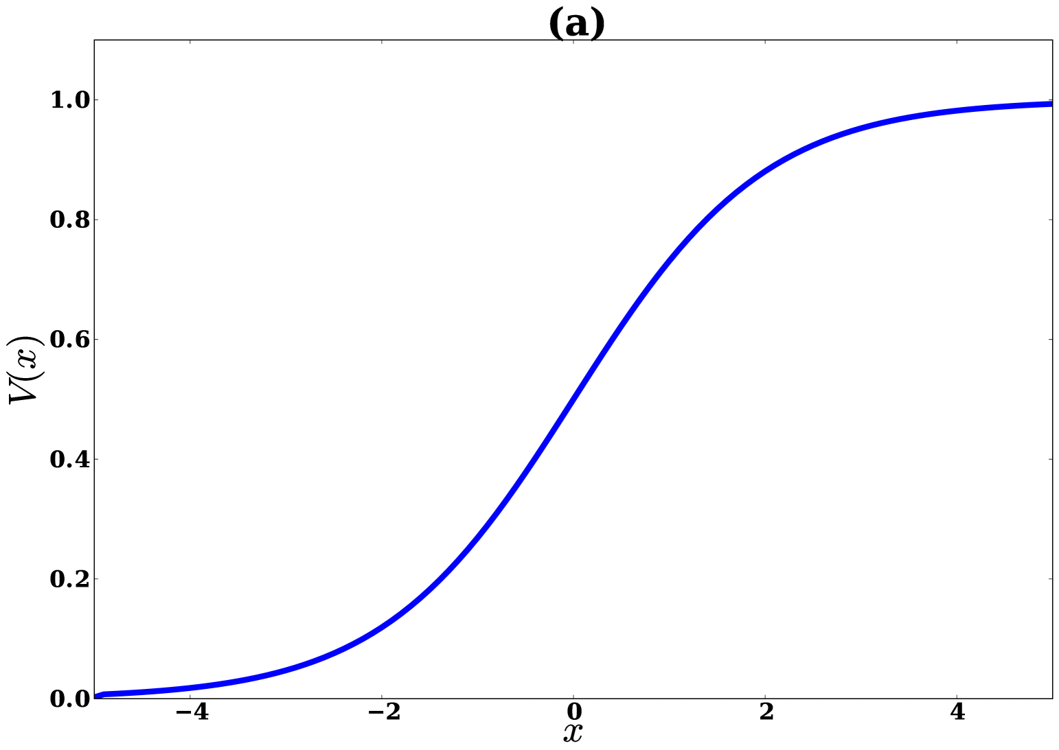
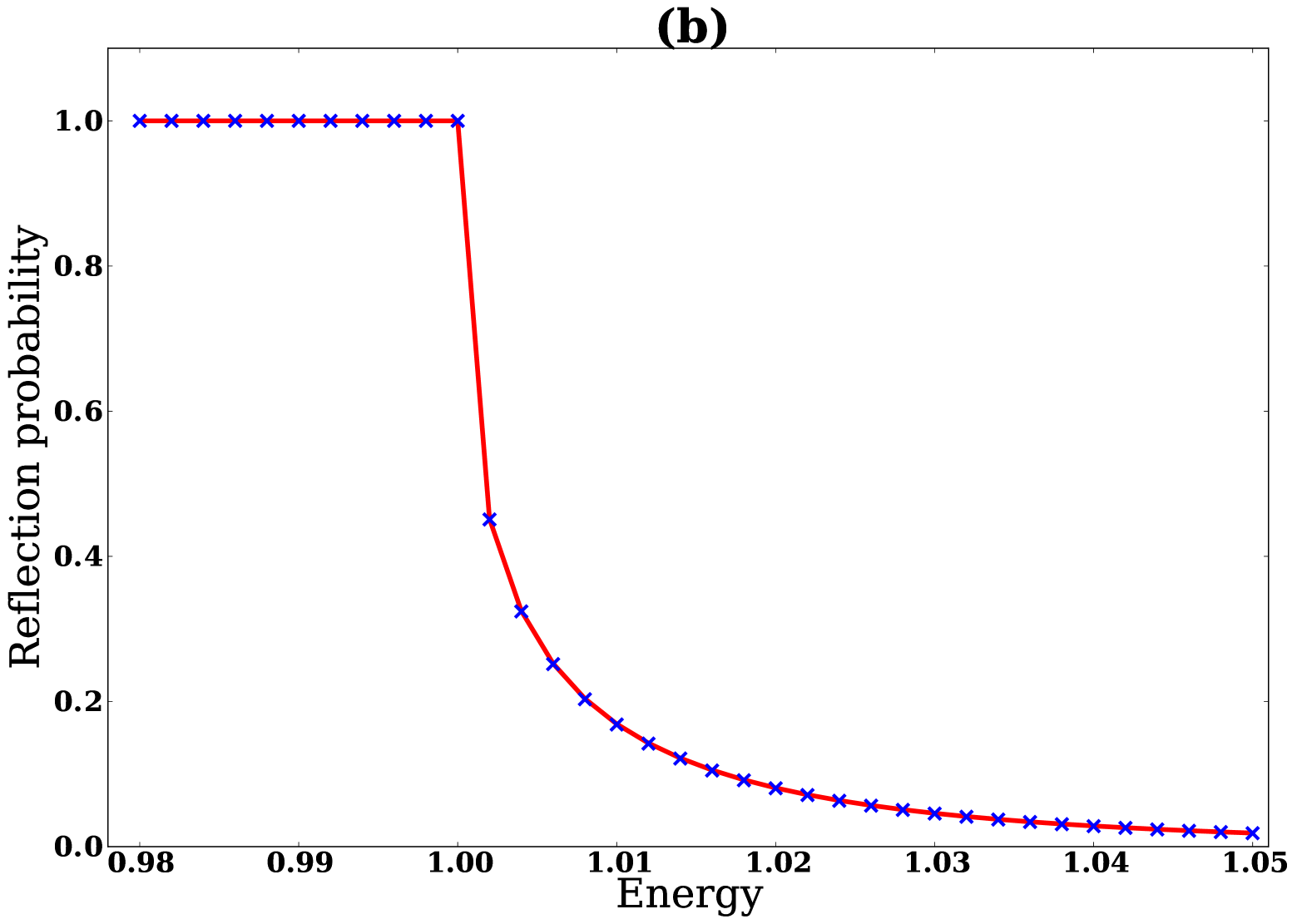
Figure 8: (a) Soft potential step (b) Reflection probability for soft potential step with step height $V_{0}=1$. Blue x marks indicate values obtained using ansatz (8) and red continuous line indicates values obtained in standard quantum mechanics.

, ,

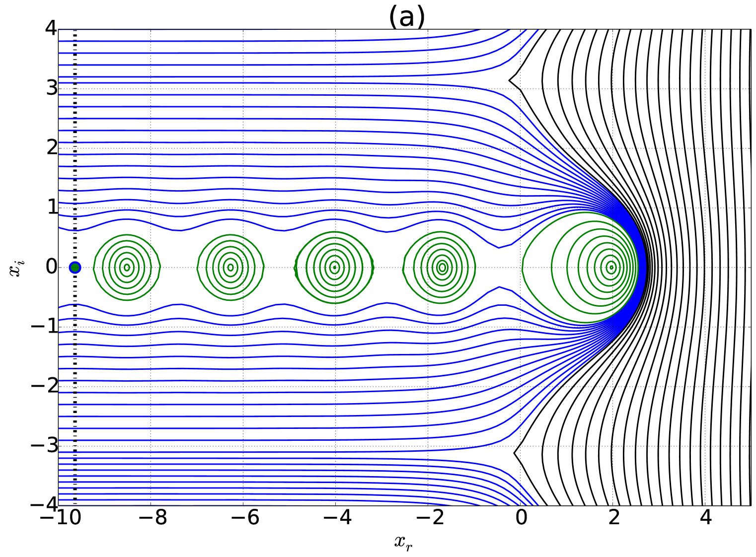
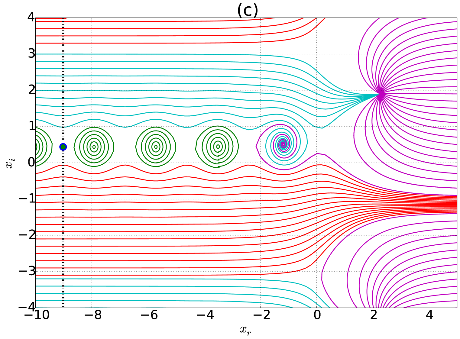
Figure 9: Complex quantum trajectories for soft potential step, for the energy values (a) $E=0.98$, (b) 1.0 and (c) 1.02. Color codes are as in Fig. 1. In each panel, the points $\alpha+i\beta$, whose numerical values are $-9.63772+0\;i$, $-9.1014+0\;i$, $-9.01653+0.440077\;i$, respectively, are marked with $\bullet$ symbols.

The reflection probability $R(k)$ obtained using the present approach and that using the standard approach flugge are plotted together in Fig. 8(b), for the values of $V_{0}=1$ and $a=1$. The agreement is very good in this case too, but when $V_{0}$ is very small, the situation can change and one may find deviations from standard results, as in the case of Eckart and Morse potentials. Another peculiarity in this case is also worth noting. The potential (16) shows periodicity, with period $2\pi a$. As the step becomes sharp with $a\rightarrow 0$, the period will be very small and consequently deviations from standard result may increase. But this type of a sharp potential step, with very small period, is different from the rectangular potential step, which has no periodicity at all mvj1 . For the soft potential step, when either $a$ or $V_{0}$ is very small, there can be deviations from standard results.

5 Conclusion

The present work is in continuation of a previous study of quantum trajectories in complex space wyatt_eckart ; wyatt_eckart1 , where among other results, the exact complex quantum trajectories for the Eckart potential barrier and the soft potential step were obtained. Plotting the complex trajectories by integrating the equation of motion $\dot{x}\equiv({1}/{m}){\partial S}/{\partial x}$, it was shown in their work that more trajectories link the left and right regions of the barrier, when the energy is increased. In the present paper, we attempt to evaluate the reflection and tunneling probabilities on the basis of these observations. It is true that these probabilities are obtained if one goes back to the standard procedure in quantum mechanics, and evaluate them using the $\psi^{\star}\psi$ distribution along the real line. But we argue that one can take the complex trajectory representation and the complex-extended probability density seriously only when it is possible to evaluate the reflection and tunneling probabilities with the help of these complex entities. Another clear motivation for the work is that the MdBB complex trajectories themselves suggest this possibility.

We have also noted that issues such as tunneling time remain as open problems in standard quantum mechanics. On the other side, in the tunneling of particles in energy eigenstates, the dBB trajectories give an unphysical prediction that all incident particles tunnel through the barrier. But as in all other predictions of observable physical quantities, the dBB approach adopts the same probability evaluation scheme used in standard quantum mechanics and claim equivalence with its results. In this paper, we investigate this issue and show that the new MdBB scheme can correctly describe the tunneling of particles in energy eigenstates and that the evaluation of reflection/tunneling probabilities can be done with the help of the complex-extended probability density and the trajectory pattern. The reflection probability is found as the ratio between the total probabilities of the reflected and the incident trajectories, the latter quantities being obtained by integrating the complex-extended probability density along the imaginary direction.

The calculations are performed for a rectangular potential barrier, symmetric Eckart and Morse barriers, and a soft potential step. It is easy to see that for the rectangular potential barrier, the agreement of $R(k)$ in Eq. (7) with the standard result $|B|^{2}/|A|^{2}$ as $\Lambda\rightarrow\infty$ shall be exact. In the case of other smooth, realistic potentials, there are slight deviations from standard results for moderate energies ($E\approx V_{0}$). These deviations arise from the periodicity of the trajectory pattern along the imaginary direction. (Since the periodicity, with constant period, is there for all $x_{r}$, the deviations cannot be attributed to the choice of $x_{r}=\alpha$, the line along which the integration is performed.) The results obtained are in very good agreement with the standard results and the predicted deviations are very small, with a maximum value only as much as $0.1\%$ of the original value. This validates the proposed complex-extended quantum probability density proposed in wyatt_prob1 ; wyatt_prob2 ; mvj_prob2 . Measurement of these small deviations shall provide an opportunity to falsify the ansatz. The new ansatz is preferred, for it is based on the characteristic feature that incident trajectories either get reflected or transmitted and that more trajectories link the left and right regions of the barrier when the energy increases. Hopefully, the new approach will lead to wide-ranging applications of the complex trajectory representation of quantum mechanics.

Acknowledgements

The authors wish to thank Prof. K. Babu Joseph and Dr. Zafar Ahmed for valuable discussions and KM wishes to thank the Santhom Computing Facility, Kozhencherry, for hospitality.

References

- (1) John, M.V.: Modified de Broglie-Bohm approach to quantum mechanics. Found. Phys. Lett. 15, 329 (2002)
- (2) Wentzel, G.: Z. Phys. 38, 518 (1926)
- (3) Pauli, W.: General Principles of Quantum Mechanics. Springer, Berlin (1980)
- (4) Dirac, P.A.M. : The Principles of Quantum Mechanics. Oxford University Press, London, (1958)
- (5) Goldstein, H.: Classical Mechanics. Addison-Wesley, Reading, MA, (1980)
- (6) de Broglie, L.: J. Phys. Rad., 6e serie, t. 8, 225 (1927)
- (7) Bacciagaluppi, G., Valentini, A.: Quantum Theory at the Crossroads. Cambridge University Press, Cambridge (2009)
- (8) Bohm, D., Hiley, B.J.: The Undivided Universe. Routledge, London and New York (1993)
- (9) Holland, P.: The Quantum Theory of Motion. Cambridge University Press, Cambridge (1993)
- (10) Sanz, A.S., Miret-Artes, S.: Comment on ”Bohmian mechanics with complex action: A new trajectory-based formulation of quantum mechanics” [J. Chem. Phys. 125, 231103, (2006)]. J. Chem. Phys. 127, 197101 (2007)
- (11) Goldfarb, Y., Degani, I., Tannor, D.J.: Response to ”Comment on ’Bohmian mechanics with complex action: A new trajectory-based formulation of quantum mechanics’ ” [J. Chem. Phys. 127, 197101 (2007)]. J. Chem. Phys. 127, 197102 (2007)
- (12) Benseny, A., Albareda, G., Sanz, A.S., Mompart, J., Oriols, X.: Applied Bohmian Mechanics. Eur. Phys. J. 68, 286 (2014)
- (13) Floyd, E.R.: Modified potential and Bohm’s quantum-mechanical potential. Phys. Rev. D 26, 1339 (1982)
- (14) Faraggi, A., Matone. M.: Quantum mechanics from an equivalence principle. Phys. Lett. B 450, 34 (1999)
- (15) Carroll, R.: Quantum Theory, Deformation, and Integrability. North Holland (2000)
- (16) Yang, C.-D.: Quantum dynamics of hydrogen atom in complex space. Ann. Phys. (N.Y.) 319, 399 (2005)
- (17) Yang, C.-D: Wave-particle duality in complex space. Ann. Phys. (N.Y.) 319, 444 (2005)
- (18) Sanz, A.S., Miret-Artes, S.: Aspects of nonlocality from a quantum trajectory perspective: A WKB approach to Bohmian mechanics. Chem. Phys. Lett. 445, 350 (2007)
- (19) Lopreore, C.L., Wyatt, R.E.:Quantum wave packet dynamics with trajectories. Phys. Rev. Lett. 82, 5190 (1999)
- (20) Goldfarb, Y., Degani, I., Tannor, D.J.: Bohmian mechanics with complex action: A new trajectory-based formulation of quantum mechanics. J. Chem. Phys. 125, 231103 (2006)
- (21) Chou, C.-C., Wyatt, R.E.: Computational method for the quantum Hamilton-Jacobi equation: One-dimensional scattering problems. Phys. Rev. E 74, 066702 (2006)
- (22) Chou, C.-C., Wyatt, R.E.: Computational method for the quantum Hamilton-Jacobi equation: Bound states in one-dimension. J. Chem. Phys. 125, 174103 (2007)
- (23) John, M.V.: Probability and complex quantum trajectories. Ann. Phys. 324, 220 (2009)
- (24) Poirier, B.: Flux continuity and probability conservation in complexified Bohmian mechanics. Phys. Rev. A 77, 022114 (2008)
- (25) Chou, C.-C., Wyatt, R.E.: Considerations on the probability density in complex space. Phys. Rev. A 78, 044101 (2008)
- (26) Chou, C.-C., Wyatt, R.E.: Arbitrary Lagrangian-Eulerian rate equation for the Born probability density in complex space. Phys. Lett. A 373, 1811 (2009)
- (27) John, M.V.: Probability and complex quantum trajectories: Finding the missing links. Ann. Phys. 325, 2132 (2010)
- (28) Flugge, S.: Practical Quantum Mechanics. Springer, New York, (1994)
- (29) Ahmed, Z.: Tunneling through a one-dimensional potential barrier. Phys. Rev. A 47, 4761 (1993)
- (30) Norsen, T.: The pilot-wave perspective on quantum scattering and tunneling. Am. J. Phys. 81, 258 (2013)
- (31) Floyd, E.R.: A trajectory interpretation of transmission and reflection. Phys. Essays 7, 135 (1994)
- (32) Chou, C.-C., Wyatt, R.E.: Quantum trajectories in complex space. Phys. Rev. A 76, 012115 (2007)
- (33) Chou, C.-C., Wyatt, R.E.: Quantum trajectories in complex space: One-dimensional stationary scattering problems. J. Chem. Phys. 128, 154106 (2008)
- (34) Rowland, B.A., Wyatt, R.E.: Analysis of barrier scattering with real and complex quantum trajectories. J. Phys. Chem. A 111, 10234 (2007)
- (35) Hartman, T.E.: Tunneling of a wave packet. J. Appl. Phys. 33, 3427 (1962)
- (36) Davies, P.C.W.: Quantum tunneling time. Am. J. Phys. 73, 23 (2005)