Holographic Brownian motion at finite density

Abstract

Brownian motion of a heavy charged particle at zero and small (but finite) temperature is studied in presence of finite density. We are primarily interested in the dynamics at (near) zero temperature which is holographically described by motion of a fundamental string in an (near-) extremal Reissner-Nordstr$\ddot{\text{o}}$m black hole. We analytically compute the functional form of retarded Green’s function for small frequencies and extract the dissipative behavior at and near zero temperature.

1 Introduction

AdS/CFT or more generally gauge/gravity duality [1, 2, 3, 4] has been serving as a great weapon in a theoretician’s armory to study strongly coupled systems analytically for almost last two decades. Although for most of the cases its predictions are qualitative, there are instances (see for example the famous $\eta/s$ computation in [5]) when it relates very formal theoretical frame work to real life experiments. Since its discovery this duality has glued many phenomena appearing in apparently different branches of physics together. Studying Brownian motion of a heavy particle using classical gravity technique is one such example [6, 7] where holography relates a statistical system to a gravitational one. The dual gravity description involves a long fundamental string stretching from the boundary of the AdS space into the black hole horizon. Numerous works [8, 9, 10, 11, 12, 13, 14, 15, 16, 17, 18] have been done elaborating on different aspects of this set-up.

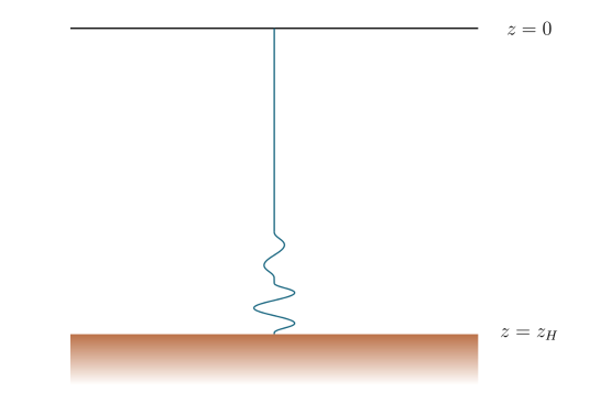
Figure 1: Gravity set up describing Brownian motion

Integrating out the whole string in that background gives an effective description of the heavy particle at the boundary. Its dynamics is governed by a Langevin equation. For a particle with mass $M$ which is moving with velocity $v$ the Langevin equation reads

$$M\frac{dv}{dt}+\gamma v=\xi(t)$$ (1.1)

$$\text{with \ \ \ }\langle \xi(t)\xi(t^{\prime})\rangle=\Gamma\delta(t-t^{\prime})$$ (1.2)

where $\gamma$ is the viscous drag, $\xi$ is the random force on the particle and $\Gamma$ quantifies the strength of the ‘noise’ (i.e, random force). The Second equation is one of the many avatars of celebrated fluctuation-dissipation theorem. One can write down a generalized version of this equation

$$M_{0}\frac{d^{2}x(t)}{dt^{2}}+\int_{-\infty}^{t}dt^{\prime}~{}G_{R}(t,t^{\prime})x(t^{\prime})=~{}\xi(t)\hskip 48.36958pt\langle\xi(t)\xi(t^{\prime})\rangle=~{}iG_{\text{sym}}(t,t^{\prime})$$ (1.3)

$G_{R}(t,t^{\prime})$ is thus the same as $\gamma(t-t^{\prime})$ for the choice of the lower limit of the integral, $t_{0}=-\infty$ and $iG_{\text{sym}}(t,t^{\prime})$ is the same as $\Gamma(t-t^{\prime})$.

In frequency space the generalized Langevin equation takes the following form

$$\left[-M_{0}\,\omega^{2}+G_{R}(\omega)\right]x(\omega)=\,\xi(\omega)\hskip 56.9055pt\langle\xi(-\omega)\,\xi(\omega)\rangle=\,i\,G_{\text{sym}}(\omega)$$ (1.4)

If the retarded Green’s function, $G_{R}(\omega)$ is expanded for small frequencies the coefficient of $\omega^{2}\left(i.e,\frac{d^{2}x(t)}{dt^{2}}\right)$ adds to the bare mass of the particle and the coefficient of $\omega\left(i.e,\frac{dx(t)}{dt}\right)$ will show off as the drag term

$$G_{R}(\omega)=-i\gamma\omega-\Delta M\omega^{2}+\ldots$$ (1.5)

After defining the ‘renormalized’ mass as

$$M\equiv M_{0}+\Delta M$$

this generalized Langevin equations (1.4) (up to $\mathcal{O}(\omega^{2})$) take the standard form (1.1) and (1.2).

From the above discussion it is quite clear that if we are interested in studying dissipation for a Brownian particle we just need to compute the retarded Green’s function, $G_{R}(\omega)$. We can calculate this quantity using different holographic techniques [19, 20] depending on the physical systems.

In [9] Brownian motion for a heavy quark in 1+1 dimensions was studied following [7] which used the prescription of [19, 21] to compute the boundary Green’s function. The calculation of [9] was performed in BTZ black hole background where the system is exactly solvable. The main result was to obtain dissipation for the heavy quark even at zero temperature. The result might look very counter intuitive and unphysical at first sight because at zero temperature the thermal fluctuations go to zero and therefore the Brownian particle should stop dissipating energy. But this zero temperature dissipation has its origin in radiation of an accelerated charged particle. The force term in the Langevin equation at zero temperature was of the form

$$F(\omega)=-i\,{\sqrt{\lambda}\over 2\pi}\,\omega^{3}\,x(\omega)$$ (1.6)

Therefore the integrated energy loss is given by

$$\Delta E={\sqrt{\lambda}\over 2\pi}\int dt\,a^{2}$$ (1.7)

It is known from classical electrodynamics that the energy loss due to radiation is proportional to square of the acceleration ($a$). See [26, 27, 28, 29, 30, 31, 32, 10, 33, 34, 35, 36, 37] for related works.

Dissipation at zero temperature is a fascinating phenomenon. Its emergence from the retarded Green’s function signifies that $G_{R}(\omega)$ actually contains information at the ‘quantum’ level (by ‘quantum’ here we mean dynamics at $T=0$). Brownian motion of a particle is usually studied at finite temperature. The system is driven by fluctuations which are thermal in nature and therefore if the temperature is taken to zero that $G_{R}(\omega)$ must vanish too. But the $G_{R}(\omega)$ we obtain from holography contains information of both thermal and quantum fluctuations for the boundary theory. Although at finite $T$ thermal fluctuations dominate over the quantum ones at very small $T$ the latter ones are much more important. The main aim of this paper is to understand how a heavy particle’s (quark’s) motion at finite density (chemical potential $\mu\neq 0$) is described at and near $T=0$. The dual gravity theory should contain an (near-) extremal charged black hole. (See [38, 39] for some results in this set up).

For high temperature regime ($\mu\ll T$) the effect of the charge of the non-extremal black hole can be neglected at the leading order and $G_{R}(\omega)$ can be computed in small $\mu$ and small $\omega$ expansions using the methods followed in [19, 7].

In this paper we would like to see how the system behaves near $T=0$. Therefore the other limit $\mu\gg T$ i.e, the low temperature regime is of more interest to us. We will see that in this regime usual perturbation techniques for small $T$ and small $\omega$ won’t work because of a double pole for the $\omega^{2}$ term in the string equation of motion in the extremal black hole background. Due to this double pole, near horizon dynamics is extremely sensitive to $\omega$. To get around this problem we will adopt the matching technique described in [20] where the authors studied non-Fermi liquids using holography.

The rest of the paper is organized as follows. In section 2 we quickly review the Reissner-Nordstr$\ddot{\text{o}}$m (RN) black hole in asymptotically AdS space time. The main purpose is to spell out the notations and conventions that we will be following through out the article. The section 3 contains the analytic computation of retarded Green’s function at zero temperature using matching technique. We also list some of its properties in detail. The retarded Green’s function at small but finite temperature is analyzed in section 4. We mainly discuss how $G_{R}(\omega)$ gets small $T$ corrections. Section 5 summarizes the main results and their interpretations, assumptions we make and some future directions. Section 6 contains some concluding remarks.

2 AdS-RN black hole background

AdS-RN black hole is a solution to Einstein-Maxwell equation with a negative cosmological constant.

$$S_{EM}=\frac{1}{2\kappa^{2}}\int d^{d+1}x\,\sqrt{-g}\,\left[R+\frac{d(d-1)}{L_{d+1}^{2}}+\frac{L_{d+1}^{2}}{g_{F}^{2}}\,F_{MN}\,F^{MN}\right]$$ (2.1)

$R$ is the Ricci scalar, $g_{F}$ is the dimensionless gauge coupling in the bulk. $L_{d+1}$ is a length scale (known as AdS radius) and $\kappa^{2}$ is Newton’s constant. Notice that we can always redefine the gauge field by absorbing the dimensionless coupling $g_{F}^{2}$ into $F_{MN}$. Thus we can fix $g_{F}$ to one without loss of generality. The (d+1) dimensional metric and gauge field that satisfy the corresponding equations of motion are given by

$$ds^{2}=\frac{L_{d+1}^{2}}{z^{2}}(-f(z)dt^{2}+d\vec{x}^{2})+\frac{L_{d+1}^{2}}{z^{2}}\frac{dz^{2}}{f(z)}$$ (2.2)

where,

$$f(z)=1+Q^{2}z^{2d-2}-Mz^{d}$$

$$A_{t}(z)=\mu(1-\frac{z^{d-2}}{z_{0}^{d-2}})$$

$Q,M,z_{0}$ are constant parameters which are black hole charge, black hole mass and horizon radius respectively. $\mu$ is the chemical potential, $\vec{x}\equiv(‎x^{1},x^{2}\ldots x^{d-1})$ and $z$ is the radial co-ordinate in the bulk such that the boundary of this space is at $z=0$.

Notice that if we put $f(z)=1$ we get back pure $AdS_{d+1}$ in Poincare patch. This non trivial function $f(z)$ indicates that the physics changes as we move along the radial direction.

At the horizon : $f(z_{0})=0$. Therefore we can express $M$ as

$$M=z_{0}^{-d}+Q^{2}z_{0}^{d-2}$$ (2.3)

Now $Q$ can be expressed in terms of chemical potential($\mu$)

$$Q=\sqrt{\frac{2(d-2)}{d-1}}\frac{\mu}{z_{0}^{d-2}}$$ (2.4)

And the Hawking temperature

$$T=\frac{d}{4\pi z_{0}}(1-\frac{d-2}{d}Q^{2}z_{0}^{2d-2})$$ (2.5)

Actually $Q,M$ and $z_{0}$ are related to charge density, energy density and entropy density in the boundary theory respectively. $Q$ is charge density up to some numbers. Lets introduce a new length scale $z_{*}$ to express $Q$ as

$$Q:=\sqrt{\frac{d}{d-2}}\frac{1}{z_{*}^{d-1}}$$ (2.6)

We also define $\mu_{*}=\frac{1}{z_{*}}$. Note that $z_{*}\geq z_{0}$ to avoid the naked singular geometry. (This is equivalent to $M\geq Q$ condition.)

There are two distinct situations possible : Extremal ($T=0$) and Non-extremal ($T\neq 0$).

2.1 Extremal black hole

When the Hawking temperature is zero the black hole is called extremal. Extremal black hole contains maximum possible charge. The “blackening function” becomes

$$f(z)=1+\frac{d}{d-2}\frac{z^{2d-2}}{z_{*}^{2d-2}}-\frac{2(d-1)}{d-2}\frac{z^{d}}{z_{*}^{d}}$$ (2.7)

Near horizon region for the extremal black hole becomes $AdS_{2}\times\mathbb{R}^{d-1}$

$$ds^{2} =\frac{L_{2}^{2}}{\zeta^{2}}(-dt^{2}+d\zeta^{2})+\mu_{*}^{2}L_{d+1}^{2}d\vec{x}^{2}$$ (2.8)

$$A_{t}(\zeta) =\frac{1}{\sqrt{2d(d-1)}}\frac{1}{\zeta}$$ (2.9)

where, $\zeta:=\frac{z_{*}^{2}}{d(d-1)(z_{*}-z)}$ , $L_{2}$ is the radius of the $AdS_{2}$ and is related to $L_{d+1}$ by the following relation

$$L_{2}=\frac{1}{\sqrt{d(d-1)}}L_{d+1}$$

2.2 Non-extremal black hole

Generically charged black holes have non-vanishing temperature. We will be interested in studying Brownian motion at finite density and finite temperature ($T$) but with $T\ll\mu$. We want to be in this regime because the near horizon geometry will become $AdS_{2}$-BH $\times\mathbb{R}^{d-1}$.

$$ds^{2} =\frac{L_{2}^{2}}{\zeta^{2}}\left(-g(\zeta)dt^{2}+\frac{d\zeta^{2}}{g(\zeta)}\right)+\mu_{*}^{2}L_{d+1}^{2}d\vec{x}^{2}$$ (2.10)

$$A_{t}(\zeta) =\frac{1}{\sqrt{2d(d-1)}}\frac{1}{\zeta}(1-\frac{\zeta}{\zeta_{0}})$$ (2.11)

where $g(\zeta):=(1-\frac{\zeta^{2}}{\zeta_{0}^{2}})$, $\zeta_{0}:=\frac{z_{*}^{2}}{d(d-1)(z_{*}-z_{0})}$ and the corresponding temperature, $T=\frac{1}{2\pi\zeta_{0}}$. For $T\approx\mu$ this nice structure breaks down.

3 Brownian motion at zero temperature

To understand Brownian motion of a heavy charged particle in some strongly coupled field theory in d-dimensions which has a gravity dual one needs to study the dynamics of a long string in the dual gravity background [6, 7]. Therefore to explore the same Brownian motion at zero temperature and finite density one needs to study a string in an extremal charged black hole. This section contains the main analysis and results of the paper.

3.1 Green’s function by matching solutions

In this Einstein-Maxwell theory an elementary string cannot couple to the gauge field, $A_{M}$. It can only couple to the background metric $G_{MN}$. We consider geometries with vanishing Kalb-Ramond field, $B_{MN}$. For this zero temperature case $G_{MN}$ can be read off from the extremal BH background (2.2) with $f(z)$ given in (2.7).

The string dynamics is given by standard Nambu-Goto action

$$S_{NG}=-\frac{1}{2\pi l_{s}^{2}}\int d\tau\,d\sigma\,\sqrt{-h}$$ (3.1)

where $l_{s}$ is the string length and $h_{ab}$ is the induced metric on the world sheet

$$h_{ab}=G_{MN}\,\partial_{a}X^{M}\,\partial_{b}X^{N}$$

We choose to work in static gauge,

$$\tau\equiv t\text{\ \ and}~{}~{}\sigma\equiv\zeta$$

Also we can choose one particular direction, say $x_{1}$ (we call this simply $x$ for brevity), along which the world sheet fluctuates.

$$x\equiv x(\tau,\sigma)=x(t,\zeta)$$

To understand the dynamics of the string we need to use the full background metric (2.2) with the “blackening factor” given in (2.7). Varying the Nambu-Goto action

$$S_{NG}=-\frac{1}{2\pi l_{s}^{2}}\int dt\,dz\,\frac{L_{d+1}}{z^{2}}\left[1+\frac{1}{2}\,f(z)\,x^{\prime 2}-\frac{1}{2f(z)}\,\dot{x}^{2}\right]$$ (3.2)

we obtain the equation of motion (EOM) in frequency space

$$x_{\omega}^{\prime\prime}(z)+\,\frac{\frac{d}{dz}(\frac{f(z)}{z^{2}})}{\frac{f(z)}{z^{2}}}\,x_{\omega}^{\prime}(z)+\frac{\omega^{2}}{[f(z)]^{2}}\,x_{\omega}(z)=0$$ (3.3)

where we have used $x(z,t)=\int\frac{d\omega}{2\pi}\,e^{-\,i\omega t}x_{\omega}(z)$

Now to obtain $G_{R}(\omega)$ the standard procedure would be to solve this equation and obtain it from the on shell action. But this procedure involves a few subtleties [20]. Firstly this differential equation is not exactly solvable. Even if we are interested in $G_{R}(\omega)$ for very small frequencies ($\omega\ll\mu$) we cannot directly perform a perturbation expansion in small $\omega$. Because at zero temperature the $f(z)$ has a double zero at the horizon (extremal limit) and consequently $\omega^{2}$ term in the equation of motion generates a double pole at the horizon. Thus this singular term dominates at the horizon irrespective of however small $\omega$ we choose.

To get around this difficulty we closely follow the matching technique in [20]. At first we isolate the ‘singular’ near horizon region from the original background. We already know that the near horizon geometry is given by $AdS_{2}\times\mathbb{R}^{d-1}$ (2.8). This is referred to as IR/inner region and the rest of the space time as UV/outer region. We can solve the string EOM exactly in this IR region and therefore the treatment will be non-perturbative in $\omega$. On the other hand the $\omega$-dependence in UV region can be treated perturbatively as there is no more $\omega$-sensitivity. The main task is to match the solutions over these two regions. The overlap between these to regions is near the boundary ($\zeta\to 0$) of the $AdS_{2}$ where

$$\frac{1}{\mu}\ll\zeta\ll\frac{1}{\omega}$$

$$\text{with}~{}~{}~{}z_{*}^{2}\frac{\omega^{2}}{f(z)}\sim\omega^{2}\zeta^{2}~{}~{}~{}\text{is very \emph{small} }$$

$$\text{and}~{}~{}~{}\mu\zeta\sim\frac{z_{*}}{z_{*}-z}~{}~{}\text{remains \emph{large}}$$

The last two expressions ensure that the $\omega$ dependent term becomes small in EOM and we are still near the horizon respectively.

$\bullet~{}~{}$ Inner region

For the string in $AdS_{2}\times\mathbb{R}^{d-1}$ (2.8)

$$\sqrt{-h} =\frac{L_{2}^{2}}{\zeta^{2}}\,\sqrt{1+\frac{L_{d+5}^{2}}{L_{2}^{2}}\,\mu_{*}^{2}\,\zeta^{2}(x^{\prime 2}-\dot{x}^{2})}$$

$$\approx\frac{L_{2}^{2}}{\zeta^{2}}\left[1+\frac{1}{2}d(d-1)\,\mu_{*}^{2}\,\zeta^{2}(x^{\prime 2}-\dot{x}^{2})\right]$$ (3.4)

The Nambu-Goto action

$$S_{NG}=-\frac{L_{2}^{2}}{2\pi l_{s}^{2}}\int dt\,d\zeta\left[\frac{1}{\zeta^{2}}+\frac{1}{2}d(d-1)\,\mu_{*}^{2}\,(x^{\prime 2}-\dot{x}^{2})\right]$$ (3.5)

Varying this action we get a very simple EOM for the string which is that of a free wave equation

$$x^{\prime\prime}-\ddot{x}=0$$ (3.6)

To solve this linear EOM, the standard way is to go to the Fourier space

$$x(\zeta,t)=\int\frac{d\omega}{2\pi}\,e^{-\,i\omega t}\,x_{\omega}(\zeta)$$ (3.7)

The equation of motion reduces to

$$x_{\omega}^{\prime\prime}(\zeta)+\omega^{2}\,x_{\omega}(\zeta)=0$$ (3.8)

This is very well known differential equation with two independent solutions

$$x_{\omega}(\zeta)=e^{\pm i\omega\zeta}$$

As we are interested in calculating retarded Green’s function we need to pick the one which is ingoing at the horizon ($\zeta\to\infty$). It’s easy to see that $e^{+\,i\omega\zeta}$ is ingoing at the horizon.

Once we pick the right solution at the horizon we need to expand that near the boundary($\zeta=0$) of the IR geometry i.e, $AdS_{2}\times\mathbb{R}^{d-1}$

$$x_{\omega}(\zeta)=1+i\omega\zeta~{},~{}~{}~{}~{}~{}~{}~{}~{}\text{near}~{}~{}\zeta=0$$ (3.9)

The ratio of normalizable to non-normalizable mode fixes the Green’s function for the IR geometry

$$\mathscr{G}_{R}(\omega)=i\omega$$ (3.10)

(We will see in (3.14) that for string in $AdS_{d+1}$ non-normalizable and normalizable modes go as $z^{0}$ and $z^{3}$ respectively. Where as in $AdS_{2}\times\mathbb{R}^{d-1}$ (3.9) they go as $z^{0}$ and $z^{1}$ .)

$\bullet~{}~{}$ Outer region

For the outer region we need to solve the full EOM (3.3). But now as we are away from the ‘dangerous’ near horizon region we can do a small frequency expansion. At the leading order we can put $\omega=0$. Let’s say that the (3.3) has two independent solutions $\eta^{(0)}_{+}$ and $\eta^{(0)}_{-}$ for $\omega=0$. We can fix there behavior near the horizon ($z=z_{*}$) and near the boundary ($z=0$) by solving this equation near those regions.

Near horizon

Near $z=z_{*}$

$$f(z)\approx d(d-1)\frac{(z_{*}-z)^{2}}{z_{*}^{2}}$$

The EOM reduces to

$$x_{\omega}^{\prime\prime}(z)-\frac{2}{z_{*}-z}~{}x_{\omega}^{\prime}(z)=0$$ (3.11)

The two independent solutions are

$$c~{}~{}\text{and}~{}~{}\frac{z_{*}}{z_{*}-z}$$

Here $c$ is some constant which can be chosen to be 1. Since we need to match the inner and the outer solutions near $z=z_{*}$ let’s express these independent solutions in terms of $\zeta$.

$$\eta^{(0)}_{+}\to\left(\frac{\zeta}{z_{*}}\right)^{0}~{}~{},~{}~{}\eta^{(0)}_{-}\to\left(\frac{\zeta}{z_{*}}\right)^{1}$$ (3.12)

Near boundary

Near the boundary, $z=0$ we can approximate $f(z)\approx 1$ and consequently the EOM

$$x_{\omega}^{\prime\prime}(z)-\frac{2}{z}~{}x_{\omega}^{\prime}(z)=0$$ (3.13)

The solutions near $z=0$ will behave as

$$\eta^{(0)}_{+} \approx a^{(0)}_{+}\left(\frac{z}{z_{*}}\right)^{0}+b^{(0)}_{+}\left(\frac{z}{z_{*}}\right)^{3}$$ (3.14)

$$\eta^{(0)}_{-} \approx a^{(0)}_{-}\left(\frac{z}{z_{*}}\right)^{0}+b^{(0)}_{-}\left(\frac{z}{z_{*}}\right)^{3}$$ (3.15)

Notice that $a^{(0)}_{\pm},b^{(0)}_{\pm}$ are not independent but related by Wronskian. We will use this information below to fix one of those coefficients.

Matching the solutions

We have some solutions to the full EOM in patches. All we need to do to obtain the Green’s function is to determine the outer solution by matching it to the inner solution in the overlap region. Then expand that solution near $z=0$ to compute the ratio of normalizable to non-normalizable mode.

Let’s do the matching first. From (3.9) and (3.12) we can express the outer solution as

$$x_{\omega}(z)=\eta^{(0)}_{+}(z)+\mathscr{G}_{R}(\omega)z_{*}\eta^{(0)}_{-}(z)$$ (3.16)

Notice that so far we have been using solutions to the UV equation which are $0^{th}$-order in $\omega$ (as we have put $\omega=0$). But in principle we can systematically add higher order corrections in $\omega$. In that improved version the outer solution will be given by

$$x_{\omega}(z) =\eta_{+}(z)+\mathscr{G}_{R}(\omega)z_{*}\eta_{-}(z)$$ (3.17)

$$\text{where}~{}~{}~{}\eta_{\pm}(z) =\eta^{(0)}_{\pm}(z)+\omega^{2}\eta^{(2)}_{\pm}(z)+\omega^{4}\eta^{(4)}_{\pm}(z)+\ldots$$ (3.18)

And as before near boundary, $z=0$

$$\eta_{\pm} \approx a_{\pm}\left(\frac{z}{z_{*}}\right)^{0}+b_{\pm}\left(\frac{z}{z_{*}}\right)^{3}$$ (3.19)

$$\text{where}~{}~{}~{}a_{\pm} =a^{(0)}_{\pm}+\omega^{2}a^{(2)}_{\pm}+\omega^{4}a^{(4)}_{\pm}+\ldots$$ (3.20)

$$~{}~{}~{}b_{\pm} =b^{(0)}_{\pm}+\omega^{2}b^{(2)}_{\pm}+\omega^{4}b^{(4)}_{\pm}+\ldots$$ (3.21)

Note that $a_{\pm},b_{\pm}$ are all real coefficients because the UV equation (3.3) and the boundary condition (3.12) at $z=z_{*}$ are both real. Also the perturbation in frequency are in even powers in $\omega$ as (3.3) contains only $\omega^{2}$.

Finally to obtain the retarded Green’s function we expand the outer solution (3.17) near the boundary($z=0$)

$$x_{\omega}(z)=A(\omega)\left(\frac{z}{z_{*}}\right)^{0}+B(\omega)\left(\frac{z}{z_{*}}\right)^{3}$$ (3.22)

$$A(\omega)=a_{+}+\mathscr{G}_{R}(\omega)\,z_{*}\,a_{-}$$

$$B(\omega)=b_{+}+\mathscr{G}_{R}(\omega)\,z_{*}\,b_{-}$$

Green’s function of the boundary theory is given by (see [7, 9, 18])

$$G_{R}(\omega):=\lim_{z\to 0}T_{0}(z)\left(-\frac{z^{2}}{L_{d+1}^{2}}\right)\frac{{x_{\omega}}^{\prime}(z)}{x_{\omega}(z)}$$ (3.23)

where

$$T_{0}(z)=\frac{1}{2\pi l_{s}^{2}}\frac{L_{d+1}^{4}}{z^{4}}\left[1+\frac{d}{d-2}\left(\frac{z}{z_{*}}\right)^{2d-2}-\frac{2(d-1)}{d-2}\left(\frac{z}{z_{*}}\right)^{d}\right],$$

is identified as local string tension which comes from the $z$-dependent normalization of the boundary action. Since we are interested in boundary Green’s function

$$T_{0}(z)\approx\frac{1}{2\pi l_{s}^{2}}\frac{L_{d+1}^{4}}{z^{4}}$$

and consequently the retarded Green’s function

$$G_{R}(\omega) \approx\lim_{z\to 0}\,-\frac{1}{2\pi l_{s}^{2}}\,\frac{L_{d+1}^{2}}{z^{2}}\,\frac{{\eta_{+}}^{\prime}(z)+\mathscr{G}_{R}(\omega)z_{*}{\eta_{-}}^{\prime}(z)}{\eta_{+}(z)+\mathscr{G}_{R}(\omega)z_{*}\eta_{-}(z)}$$

$$=\lim_{z\to 0}\,-\frac{L_{d+1}^{2}}{2\pi l_{s}^{2}}\,\frac{1}{z^{2}}\,\frac{3b_{+}(\frac{z}{z_{*}})^{2}\frac{1}{z_{*}}+\mathscr{G}_{R}(\omega)3b_{-}(\frac{z}{z_{*}})^{2}}{[a_{+}+\mathscr{G}_{R}(\omega)z_{*}a_{-}]+[b_{+}+\mathscr{G}_{R}(\omega)z_{*}b_{-}](\frac{z}{z_{*}})^{3}}$$

$$=-\frac{\sqrt{\lambda}}{2\pi}\,\frac{3}{z_{*}^{3}}\,\left[\frac{b_{+}+\mathscr{G}_{R}(\omega)z_{*}b_{-}}{a_{+}+\mathscr{G}_{R}(\omega)z_{*}a_{-}}\right]$$ (3.24)

We have introduced a dimensionless quantity $\lambda:=\frac{L_{d+1}^{4}}{l_{s}^{4}}$ which behaves like a coupling constant in the boundary field theory. Since we are working in supergravity limit in the bulk $L_{d+1}\gg l_{s}$ and therefore $\lambda\gg 1$ i.e, the boundary theory is strongly coupled. The expression (3.24) is the main result of this paper. Below we analyze this in detail.

3.2 Properties of the Green’s function

• The expression (3.24) depends on two sets of data.

  1. {$a_{\pm},b_{\pm}$ } : These constants come from solving EOM in the outer region. Therefore they depend on the geometry of the outer region. In this sense they are non-universal UV data.

  2. $\mathscr{G}_{R}(\omega)$ : This depends only on the IR region which always contains $AdS_{2}$ independent of the full UV theory. This is universal IR data.

  
  

• As we have already pointed out the UV data ($a_{\pm},b_{\pm}$) are always real. Whereas the IR data ($\mathscr{G}_{R}(\omega)$) is in general complex. Therefore the dissipation is always controlled by the IR data. Actually all non-analytic behavior enters into $G_{R}(\omega)$ from $\mathscr{G}_{R}(\omega)$.

  
  

• In principle $a^{(2n)}_{\pm},b^{(2n)}_{\pm}$ are fixed by (numerically) solving the EOM in UV region in $\omega^{2}$ perturbation.

  
  

• The interesting thing to notice is that the (3.3) with $\omega=0$ allows a constant solution. From the boundary condition (3.12) at $z=z_{*}$, we see that

  $$\eta_{+}^{(0)}=1$$

  This value of $\eta_{+}^{(0)}$ will continue to solve the EOM (3.3) with $\omega=0$ for the outer region $z_{*}\geq z\geq 0$. So near the boundary ($z=0$) we have (from (3.19))

  $$\eta_{+} \approx a^{(0)}_{+}\left(\frac{z}{z_{*}}\right)^{0}+b^{(0)}_{+}\left(\frac{z}{z_{*}}\right)^{3}=1$$ (3.25)

  This fixes

  $$a^{(0)}_{+}=1$$

  $$b^{(0)}_{+}=0$$

  Actually we can fix one more coefficient by equating the generalized Wronskian at the boundary and at the horizon. We get (see Appendix A for details)

  $$b_{-}^{(0)}=\frac{1}{3}$$

  The $0^{th}$-order Green’s function reduces to

  $$G_{R}^{(0)}(\omega) =-\frac{L_{d+1}^{2}}{2\pi l_{s}^{2}}\,\frac{3}{z_{*}^{3}}\,\frac{b^{(0)}_{+}+\mathscr{G}_{R}(\omega)z_{*}b^{(0)}_{-}}{a^{(0)}_{+}+\mathscr{G}_{R}(\omega)z_{*}a^{(0)}_{-}}$$

  $$=-\frac{\sqrt{\lambda}}{2\pi}\,\frac{i\mu_{*}^{2}~{}\omega}{(1+i\frac{\omega}{\mu_{*}}\,a^{(0)}_{-})}$$ (3.26)

  

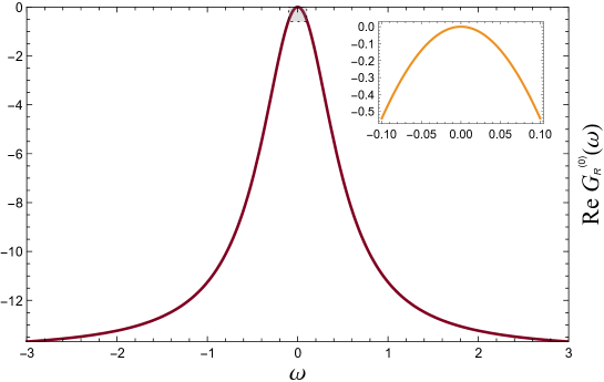
  Figure 2: Real part of $G_{R}^{(0)}(\omega)$ with $\mu_{*}=5$

  The form of $G_{R}^{(0)}(\omega)$ ensures

  $$G_{R}^{(0)}(\omega)=0~{}~{}~{}~{}~{}~{}~{}\text{as}~{}~{}\omega\to 0$$

  The real and imaginary parts of $G_{R}^{(0)}(\omega)$ are plotted (see Fig. 2 and Fig. 3) for particular values of the parameters : $\lambda=50,~{}\mu_{*}=5$ and $a^{(0)}_{-}=10$.
  

  For small frequency

  $$G_{R}^{(0)}(\omega) =-i\frac{\sqrt{\lambda}}{2\pi}\,\mu_{*}^{2}\,\omega(1-i\frac{\omega}{\mu_{*}}\,a^{(0)}_{-}+\ldots)$$

  $$\approx-i\,\frac{\sqrt{\lambda}}{2\pi}\,\mu_{*}^{2}~{}\omega-a^{(0)}_{-}\,\frac{\sqrt{\lambda}}{2\pi}\,\mu_{*}\,\omega^{2}$$ (3.27)

  

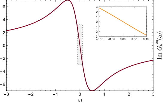
  Figure 3: Imaginary part of $G_{R}^{(0)}(\omega)$ with $\mu_{*}=5$

  This is also consistent with Langevin equation (1.5) as $G_{R}(\omega)$ expansion starts with $-i\omega$. Note that, for small frequencies, the zero temperature dissipation goes linear in $\omega$ (see Fig. 3) unlike $\mu=0$ case [9, 18] where this goes as $\omega^{3}$. The fact that $G_{R}(\omega)$ is linear in $\omega$ comes from the fact that the effective $AdS_{2}$ dimension (which can be read off from (3.12)) of the ‘quark operator’ is one (i.e. $\Delta=1$).
  

  The leading dissipative term is proportional to $\mu_{*}^{2}$. This result indicates that energy loss for the charged Brownian particle is more for medium with higher charge density.

4 Brownian motion at finite temperature

To study Brownian motion at finite but very small temperature we need to follow the same steps as before. But now the inner region will become a non-extremal (rather near extremal) black hole (2.2) background.

4.1 Green’s function by matching solutions

In this section we will go through the same procedure of matching functional form of the solutions in inner and outer regions. There will be few modifications to the zero temperature $G_{R}(\omega)$.

$\bullet~{}~{}$ Inner region

The metric in this region is black hole in $AdS_{2}\times\mathbb{R}^{d-1}$ (2.10).

The Nambu-Goto action

$$S_{NG}=-\frac{L_{2}^{2}}{2\pi l_{s}^{2}}\int dt\,d\zeta\left[\frac{1}{\zeta^{2}}+\frac{1}{2}d(d-1)\,\mu_{*}^{2}\,\left(g(\zeta)x^{\prime 2}-\frac{1}{g(\zeta)}\dot{x}^{2}\right)\right]$$ (4.1)

Varying this action we obtain the EOM in frequency space

$$x_{\omega}^{\prime\prime}(\zeta)+\,\frac{2\,\zeta}{\zeta^{2}-\zeta_{0}^{2}}\,x_{\omega}^{\prime}(\zeta)+\frac{\zeta_{0}^{4}\,\omega^{2}}{(\zeta^{2}-\zeta_{0}^{2})^{2}}\,x_{\omega}(\zeta)=0$$ (4.2)

This EOM can be solved exactly. The two independent solutions are :

$$x_{\omega}(\zeta)=e^{\pm\,i\,\zeta_{0}\,\omega\,\tanh^{-1}\left(\frac{\zeta}{\zeta_{0}}\right)}$$

Again we are interested in retarded Green’s function so we pick the solution which is ingoing at the horizon ($\zeta=\zeta_{0}$)

$$e^{+\,i\,\zeta_{0}\,\omega\,\tanh^{-1}\left(\frac{\zeta}{\zeta_{0}}\right)}$$

.

Once we have the ingoing solution we need to expand it near the boundary($\zeta=0$) of near horizon geometry

$$x^{R}_{\omega}(\zeta)=1+i\,\omega\,\zeta$$ (4.3)

We can now read off the Green’s function in IR region

$$\mathscr{G}_{R,T}(\omega)=i\,\omega$$ (4.4)

This is identical to the zero temperature case (3.10).

We have discussed earlier the dissipative part of $G_{R}(\omega)$ comes solely from the IR Green’s function. For this particular problem $\mathscr{G}_{R,T}(\omega)=\mathscr{G}_{R}(\omega)=i\omega$. Therefore $T$-dependence can only creep in via the expansion coefficients ($a_{\pm},b_{\pm}$).

$\bullet~{}~{}$ Outer region

This outer region analysis will be almost identical to that of the zero temperature case. One just has to be careful about the coefficients ($a_{\pm},b_{\pm}$) which are now temperature dependent, in general. Therefore we can skip repeating the analysis and directly write down the Green’s function at finite temperature following the zero temperature case (see section 3)

$$G_{R,T}(\omega) =-\frac{\sqrt{\lambda}}{2\pi}\,\frac{3}{z_{*}^{3}}\,\left[\frac{b_{+}(\omega,T)+\mathscr{G}_{R,T}(\omega)\,z_{*}\,b_{-}(\omega,T)}{a_{+}(\omega,T)+\mathscr{G}_{R,T}(\omega)\,z_{*}\,a_{-}(\omega,T)}\right]$$

$$=-\frac{\sqrt{\lambda}}{2\pi}\,\frac{3}{z_{*}^{3}}\,\left[\frac{b_{+}(\omega,T)+i\,\omega\,z_{*}~{}b_{-}(\omega,T)}{a_{+}(\omega,T)+i\,\omega\,z_{*}\,a_{-}(\omega,T)}\right]$$ (4.5)

If we consider only the leading order in $\omega$ (i.e, putting $\omega=0$ in the EOM), even for the non-extremal case, $x_{\omega}=const.$ is again a solution. As before we can normalize it to one. By the same argument as in zero temperature case

$$a^{(0)}_{+}=1$$

$$b^{(0)}_{+}=0$$

Therefore the leading order Green’s function is identical to that of zero temperature case (• ‣ 3.2)

$$G_{R,T}^{(0)}(\omega)=-\frac{\sqrt{\lambda}}{2\pi}\,\frac{i\mu_{*}^{2}~{}\omega}{(1+i\frac{\omega}{\mu_{*}}\,a^{(0)}_{-})}$$ (4.6)

This Green’s function can be improved by solving the (3.3) perturbatively in $\omega$ and $T$. Actually the corrections will be in powers of $\frac{\omega}{\mu_{*}}$ and $\frac{T}{\mu_{*}}$. The corresponding real coefficients can also be obtained numerically in a systematic fashion.

5 Discussions

We have studied in detail the important properties of the retarded Green’s function we obtained from the matching technique. It has a nice structure in terms of frequency (and also in temperature). We discussed that the dissipative (in general non-analytic) part of the system is determined by the near horizon behavior i.e, the IR data of the system. On the other hand the near boundary behavior i.e the UV data is always some analytic expansion in nature. Actually these facts are compatible with our field theoretic and geometric intuitions.

For generic many body systems we know that IR physics can show non-analytic behavior but UV physics can only give analytic corrections to that. From Renormalization Group (RG) point of view this matching technique can be thought of as matching UV to IR physics at some intermediate energy scale fixed by the chemical potential ($\mu_{*}$).

Geometrically also this is expected. Dissipation is caused due to energy or ‘modes’ disappearing into “something”. In the bulk picture this can only happen near the horizon of a black hole where the modes fall into the black hole and never come back. Whereas near boundary geometry is very smooth and therefore no non-analytic behavior can be expected from that UV region.

It is worth mentioning that the leading order dissipative term at zero temperature is linear in frequency unlike the zero density situations [18, 9] where it starts with cubic term ($\omega^{3}$). Therefore this is actually the drag term associated to the velocity of the charged particle rather than the acceleration of the same. A particle moving at constant velocity at zero temperature can dissipate energy for this set-up since the presence of finite charge density breaks Lorentz symmetry of the boundary theory explicitly. Nevertheless there will be dissipation due to acceleration of the charged particle as radiation at the subleading order. Expanding $G_{R}^{(0)}(\omega)$ (• ‣ 3.2) in small frequency one can obtain the Bremsstrahlung function $B(\lambda)$ by collecting the coefficient of $\omega^{3}$.

$$B(\lambda)=\frac{\sqrt{\lambda}}{2\pi}\ {(a^{(0)}_{-})}^{2}$$

$a^{(0)}_{-}$ can be fixed by numerical technique. But this is obtained solving the string EOM (3.3) only upto $\mathcal{O}(\omega^{0})$. It will get corrections for higher orders in $\omega^{2}$ that can be taken into account systematically.

For a particular theory at finite density but at zero temperature if one can independently compute the Bremsstrahlung function, then that can be compared with the result obtained in our method. The standard and well known method of computing the Bremsstrahlung function is using supersymmetric localization technique (see e.g, [36, 24, 37]). But one would face following challenges to apply this technique at finite density. Firstly one needs to, if possible, turn on background fields corresponding to finite density while preserving enough supersymmetry. Secondly, and more specific to the computation of the Bremsstrahlung function, finite density breaks conformal invariance. Some of the steps in computing the Bremsstrahlung function use explicitly conformal symmetry. Although the Bremsstrahlung function must exist for non-conformal theories, it may no longer be controlled by localization.

The method we have used to obtain the Green’s function only required an $AdS_{2}$ factor near the horizon. Therefore it should work even if the UV theory is non-conformal (not asymptotically AdS) but the IR geometry has a $AdS_{2}$ factor. For example, instead of D3 branes one can look at D2 or D4 brane geometries. They are non-conformal [44]. If for some charge density they flow to some $AdS_{2}$ then this procedure can be applied. Also, by the same argument, it can possibly work for some rotating extremal black hole backgrounds too.

All our results are valid for large chemical potential and small temperature. If one is interested in studying Brownian motion in the opposite regime this technique can not be used. The reason being for $\mu\sim T$ the ‘nice’ inner region structure breaks down. In that case the small $\mu$ corrections can be computed using same tecniques used in [7, 9] but for a charged black hole background in AdS with very small charge.

6 Conclusions

In this paper we have used holographic technique to study Langevin dynamics of a heavy particle moving at finite charge density. We have studied this by computing retarded Green’s function via solution matching technique. Here are the main results.

• Analytic form of retarded Green’s function for small frequencies has been obtained at zero temperature.
  

• The drag force at zero temperature shows up as the leading contribution at small frequencies.
  

• It is also been sketched how the retarded Green’s function gets corrections due to small (but finite) temperature. The leading dissipative part (drag) remains identical to that in the zero temperature case.
  

• The drag term grows quadratically with the chemical potential i.e, loss in energy of the Brownian particle is more for medium with higher charge density.
  

• The leading contribution to the Bremsstrahlung function $B(\lambda)$ is obtained with an unknown co-efficient $a^{(0)}_{-}$ which can be fixed by numerical method. Its corrections in $\frac{\omega}{\mu_{*}}$ and $\frac{T}{\mu_{*}}$ can be computed systematically.

Acknowledgments

PB is grateful to B. Sathiapalan for fruitful discussions, suggestions on the manuscript and encouragement. He acknowledges useful conversation with Roberto Emparan, Tomeu Fiol and Carlos Hoyos. The author also would like to thank Rusa Mandal for helping with Mathematica.

Appendix A Fixing coefficient using generalized Wronskian

A field $\psi(z)$ satisfying a second order linear homogeneous differential equation

$$\psi^{\prime\prime}(z)+P(z)\psi^{\prime}(z)+Q(z)\psi(z)=0$$ (A.1)

where $P(z)$ and $Q(z)$ are real the generalized Wronskian is defined as

$$W(\psi_{1},\psi_{2};z) :=e^{\int^{z}P(t)dt}[\psi_{1}\partial_{z}\psi_{2}-\psi_{2}\partial_{z}\psi_{1}]$$ (A.2)

$$=\sqrt{-g}g^{zz}[\psi_{1}\partial_{z}\psi_{2}-\psi_{2}\partial_{z}\psi_{1}]$$ (A.3)

where $\psi_{1}$ and $\psi_{2}$ are two solutions of (A.1). The interesting fact about this $W(z)$ is it is independent of $z$

$$\partial_{z}W(\psi_{1},\psi_{2};z)=0.$$

Therefore we can write

$$W(\psi_{1},\psi_{2};z)\equiv W(\psi_{1},\psi_{2})$$

Equation (3.3) is exactly of the form (A.1). We know how its two independent solutions behave at the horizon ($z=z_{*}$) and at the boundary ($z=0$). The generalized Wronskian

$$W(\psi_{1},\psi_{2}) =\left(\frac{L_{d+1}^{2}}{z^{2}}\right)^{\frac{d+1}{2}}\frac{f(z)}{L_{d+1}^{2}}z^{2}(\psi_{1}\partial_{z}\psi_{2}-\psi_{2}\partial_{z}\psi_{1})$$ (A.4)

$$=\left(\frac{L_{d+1}}{z}\right)^{d-1}(\psi_{1}\partial_{z}\psi_{2}-\psi_{2}\partial_{z}\psi_{1})$$ (A.5)

is independent of $z$. Therefore

$$W(\psi_{1},\psi_{2})\bigg{|}_{z=0}=W(\psi_{1},\psi_{2})\bigg{|}_{z=z_{*}}$$ (A.6)

Now for extremal case

$$f(z)=1+\frac{d}{d-2}\left(\frac{z}{z_{*}}\right)^{2}-\frac{2d-2}{d-2}\left(\frac{z}{z_{*}}\right)^{d}$$

• $f(z)\big{|}_{z=0}=1$
  

• $f(z)\big{|}_{z=z_{*}}\approx d(d-1)\frac{(z_{*}-z)^{2}}{z_{*}^{2}}$

$$\text{LHS of \eqref{B:W-match} : }~{}~{}~{}W(\psi_{1},\psi_{2})\bigg{|}_{z=0} =\frac{1}{z^{2}}(\eta_{+}^{(0)}\partial_{z}\eta_{-}^{(0)}-\eta_{-}^{(0)}\partial_{z}\eta_{+}^{(0)})$$

$$=\frac{3}{z_{*}^{3}}(a_{+}^{(0)}b_{-}^{(0)}-a_{-}^{(0)}b_{+}^{(0)})$$ (A.7)

$$\text{RHS of \eqref{B:W-match} : }~{}~{}~{}W(\psi_{1},\psi_{2})\bigg{|}_{z=z_{*}} =\frac{d(d-1)(z_{*}-z)^{2}}{z^{2}z_{*}^{2}}(\eta_{+}^{(0)}\partial_{z}\eta_{-}^{(0)}-\eta_{-}^{(0)}\partial_{z}\eta_{+}^{(0)})$$

$$=\frac{d(d-1)(z_{*}-z)^{2}}{z^{2}z_{*}^{2}}\left[1.~{}\partial_{z}\left(\frac{\zeta}{z_{*}}\right)-\left(\frac{\zeta}{z_{*}}\right)\partial_{z}(1)\right]$$

$$=\frac{1}{z_{*}^{3}}$$ (A.8)

Equating (A) and (A)

$$a_{+}^{(0)}b_{-}^{(0)}-a_{-}^{(0)}b_{+}^{(0)}=\frac{1}{3}$$

and substituting $b_{+}^{(0)}=0$ and $a_{+}^{(0)}=1$ we get

$$b_{-}^{(0)}=\frac{1}{3}$$

References

- [1] J. M. Maldacena, The Large N limit of superconformal field theories and supergravity, Int. J. Theor. Phys. 38 (1999) 1113–1133, arXiv:hep-th/9711200 [hep-th]. [Adv. Theor. Math. Phys.2,231(1998)].
- [2] S. S. Gubser, I. R. Klebanov, and A. M. Polyakov, Gauge theory correlators from noncritical string theory, Phys. Lett. B428 (1998) 105–114, arXiv:hep-th/9802109 [hep-th].
- [3] E. Witten, Anti-de Sitter space and holography, Adv. Theor. Math. Phys. 2 (1998) 253–291, arXiv:hep-th/9802150 [hep-th].
- [4] E. Witten, Anti-de Sitter space, thermal phase transition, and confinement in gauge theories, Adv. Theor. Math. Phys. 2 (1998) 505–532, arXiv:hep-th/9803131 [hep-th].
- [5] G. Policastro, D. T. Son, and A. O. Starinets, The Shear viscosity of strongly coupled N=4 supersymmetric Yang-Mills plasma, Phys. Rev. Lett. 87 (2001) 081601, arXiv:hep-th/0104066 [hep-th].
- [6] J. de Boer, V. E. Hubeny, M. Rangamani, and M. Shigemori, Brownian motion in AdS/CFT, JHEP 07 (2009) 094, arXiv:0812.5112 [hep-th].
- [7] D. T. Son and D. Teaney, Thermal Noise and Stochastic Strings in AdS/CFT, JHEP 07 (2009) 021, arXiv:0901.2338 [hep-th].
- [8] C. P. Herzog, A. Karch, P. Kovtun, C. Kozcaz, and L. G. Yaffe, Energy loss of a heavy quark moving through N=4 supersymmetric Yang-Mills plasma, JHEP 07 (2006) 013, arXiv:hep-th/0605158 [hep-th].
- [9] P. Banerjee and B. Sathiapalan, Holographic Brownian Motion in 1+1 Dimensions, Nucl. Phys. B884 (2014) 74–105, arXiv:1308.3352 [hep-th].
- [10] E. Caceres, M. Chernicoff, A. Guijosa, and J. F. Pedraza, Quantum Fluctuations and the Unruh Effect in Strongly-Coupled Conformal Field Theories, JHEP 06 (2010) 078, arXiv:1003.5332 [hep-th].
- [11] S. Chakrabortty, S. Chakraborty, and N. Haque, Brownian motion in strongly coupled, anisotropic Yang-Mills plasma: A holographic approach, Phys. Rev. D89 no. 6, (2014) 066013, arXiv:1311.5023 [hep-th].
- [12] S. S. Gubser, Momentum fluctuations of heavy quarks in the gauge-string duality, Nucl. Phys. B790 (2008) 175–199, arXiv:hep-th/0612143 [hep-th].
- [13] J. Casalderrey-Solana and D. Teaney, Transverse Momentum Broadening of a Fast Quark in a N=4 Yang Mills Plasma, JHEP 04 (2007) 039, arXiv:hep-th/0701123 [hep-th].
- [14] W. Fischler, P. H. Nguyen, J. F. Pedraza, and W. Tangarife, Fluctuation and dissipation in de Sitter space, JHEP 08 (2014) 028, arXiv:1404.0347 [hep-th].
- [15] D. Giataganas and H. Soltanpanahi, Universal Properties of the Langevin Diffusion Coefficients, Phys. Rev. D89 no. 2, (2014) 026011, arXiv:1310.6725 [hep-th].
- [16] D. Giataganas and H. Soltanpanahi, Heavy Quark Diffusion in Strongly Coupled Anisotropic Plasmas, JHEP 06 (2014) 047, arXiv:1312.7474 [hep-th].
- [17] D. Roychowdhury, Quantum fluctuations and thermal dissipation in higher derivative gravity, Nucl. Phys. B897 (2015) 678–696, arXiv:1506.04548 [hep-th].
- [18] P. Banerjee and B. Sathiapalan, Zero Temperature Dissipation and Holography, JHEP 04 (2016) 089, arXiv:1512.06414 [hep-th].
- [19] D. T. Son and A. O. Starinets, Minkowski space correlators in AdS / CFT correspondence: Recipe and applications, JHEP 09 (2002) 042, arXiv:hep-th/0205051 [hep-th].
- [20] T. Faulkner, H. Liu, J. McGreevy, and D. Vegh, Emergent quantum criticality, Fermi surfaces, and AdS(2), Phys. Rev. D83 (2011) 125002, arXiv:0907.2694 [hep-th].
- [21] C. P. Herzog and D. T. Son, Schwinger-Keldysh propagators from AdS/CFT correspondence, JHEP 03 (2003) 046, arXiv:hep-th/0212072 [hep-th].
- [22] D. J. Griffiths, Introduction to Electrodynamics (3rd Edition). 2009.
- [23] A. Mikhailov, Nonlinear waves in AdS / CFT correspondence, arXiv:hep-th/0305196 [hep-th].
- [24] A. Lewkowycz and J. Maldacena, Exact results for the entanglement entropy and the energy radiated by a quark, JHEP 05 (2014) 025, arXiv:1312.5682 [hep-th].
- [25] A. M. Polyakov, Gauge Fields as Rings of Glue, Nucl. Phys. B164 (1980) 171–188.
- [26] M. Chernicoff and A. Guijosa, Acceleration, Energy Loss and Screening in Strongly-Coupled Gauge Theories, JHEP 06 (2008) 005, arXiv:0803.3070 [hep-th].
- [27] M. Chernicoff, J. A. Garcia, and A. Guijosa, Generalized Lorentz-Dirac Equation for a Strongly-Coupled Gauge Theory, Phys. Rev. Lett. 102 (2009) 241601, arXiv:0903.2047 [hep-th].
- [28] M. Chernicoff, J. A. Garcia, and A. Guijosa, A Tail of a Quark in N=4 SYM, JHEP 09 (2009) 080, arXiv:0906.1592 [hep-th].
- [29] M. Chernicoff, A. Guijosa, and J. F. Pedraza, The Gluonic Field of a Heavy Quark in Conformal Field Theories at Strong Coupling, JHEP 10 (2011) 041, arXiv:1106.4059 [hep-th].
- [30] M. Chernicoff, J. A. Garcia, A. Guijosa, and J. F. Pedraza, Holographic Lessons for Quark Dynamics, J. Phys. G39 (2012) 054002, arXiv:1111.0872 [hep-th].
- [31] B.-W. Xiao, On the exact solution of the accelerating string in AdS(5) space, Phys. Lett. B665 (2008) 173–177, arXiv:0804.1343 [hep-th].
- [32] Y. Hatta, E. Iancu, A. H. Mueller, and D. N. Triantafyllopoulos, Radiation by a heavy quark in N=4 SYM at strong coupling, Nucl. Phys. B850 (2011) 31–52, arXiv:1102.0232 [hep-th].
- [33] T. Fulton and F. Rohrlich, Classical radiation from a uniformly accelerated charge, Annals of Physics 9 (1960) 499.
- [34] D. G. Boulware, Radiation From a Uniformly Accelerated Charge, Annals Phys. 124 (1980) 169.
- [35] D. Correa, J. Henn, J. Maldacena, and A. Sever, An exact formula for the radiation of a moving quark in N=4 super Yang Mills, JHEP 06 (2012) 048, arXiv:1202.4455 [hep-th].
- [36] B. Fiol, B. Garolera, and A. Lewkowycz, Exact results for static and radiative fields of a quark in N=4 super Yang-Mills, JHEP 05 (2012) 093, arXiv:1202.5292 [hep-th].
- [37] B. Fiol, E. Gerchkovitz, and Z. Komargodski, Exact Bremsstrahlung Function in Superconformal Field Theories, Phys. Rev. Lett. 116 no. 8, (2016) 081601, arXiv:1510.01332 [hep-th].
- [38] M. Edalati, J. F. Pedraza, and W. Tangarife Garcia, Quantum Fluctuations in Holographic Theories with Hyperscaling Violation, Phys. Rev. D87 no. 4, (2013) 046001, arXiv:1210.6993 [hep-th].
- [39] M. Ahmadvand and K. B. Fadafan, Energy loss at zero temperature from extremal black holes, arXiv:1512.05290 [hep-th].
- [40] I. R. Klebanov, World volume approach to absorption by nondilatonic branes, Nucl. Phys. B496 (1997) 231–242, arXiv:hep-th/9702076 [hep-th].
- [41] J. M. Maldacena and A. Strominger, Black hole grey body factors and d-brane spectroscopy, Phys. Rev. D55 (1997) 861–870, arXiv:hep-th/9609026 [hep-th].
- [42] M. Spradlin and A. Strominger, Vacuum states for AdS(2) black holes, JHEP 11 (1999) 021, arXiv:hep-th/9904143 [hep-th].
- [43] T. Faulkner, N. Iqbal, H. Liu, J. McGreevy, and D. Vegh, Holographic non-Fermi liquid fixed points, Phil. Trans. Roy. Soc. A 369 (2011) 1640, arXiv:1101.0597 [hep-th].
- [44] N. Itzhaki, J. M. Maldacena, J. Sonnenschein, and S. Yankielowicz, Supergravity and the large N limit of theories with sixteen supercharges, Phys. Rev. D58 (1998) 046004, arXiv:hep-th/9802042 [hep-th].