Non-constant ponderomotive energy in above threshold ionization by intense short laser pulses

Abstract

We analyze the contribution of the quiver kinetic energy acquired by an electron in an oscillating electric field to the energy balance in atomic ionization processes by a short laser pulse. Due to the time dependence of this additional kinetic energy, a temporal average is assumed to maintain a stationary energy conservation rule. This rule is used to predict the position of the peaks observed in the photo electron spectra (PE). For a flat top pulse envelope, the mean value of the quiver energy over the whole pulse leads to the concept of ponderomotive energy $U_{p}$. However for a short pulse with a fast changing field intensity a stationarity approximation could not be precise.

We check these concepts by studying first the photoelectron (PE) spectrum within the Semiclassical Model (SCM) for a multiple steps pulses. The SCM offers the possibility to establish a connection between emission times and the PE spectrum in the energy domain. We show that PE substructures stem from ionization at different times mapping the pulse envelope. We also present the analysis of the PE spectrum for a realistic sine-squared envelope within the Coulomb-Volkov and ab initio calculations solving the time-dependent Schrödinger equation. We found that the electron emission amplitudes produced at different times interfere with each other and produce a new additional pattern, that overlap the above-threshold ionization (ATI) peaks.

I Introduction

Above Threshold Ionization (ATI) processes have been extensively studied in the context of strong laser-matter interaction since their first observation Agostini:79 ; DiMauro:95 . In these processes the target absorbs more photons than the minimum number required for ionization and the photo-electron (PE) spectra are characterized by peaks at electron energy values $E_{n}$ assumed to be given by an energy conservation rule Parker:96

$$E_{n}+U_{p}=n\hbar\omega-I_{p},$$ (1)

where $\omega$ is the dominant laser frequency, $n$ the number of absorbed photons, $I_{p}$ is the atomic ionization potential, and $U_{p}$ is the denominated ponderomotive energy. This equation implicitly assumes that the electron ejected from a stationary state with bound energy $-I_{p}$ reaches the atomic continuum state with a defined energy determined by the action of the laser field. However, as the Hamiltonian introduced by the laser is time dependent, the electron final state energy is not precisely defined. For a long pulse with uniform envelope, the stationarity of the electron state can be approximately reconstituted by assuming that electron quiver energy in the oscillating field can be averaged over the optical cycles of the pulse resulting in the ponderomotive energy. In particular, it is well known that for an infinite flat-top pulse the ponderomotive energy reduces to $U_{p}=\left(F_{0}/2\omega\right)^{2}$, where $F_{0}$ is the laser field amplitude. However, the concept of $U_{p}$ seems not clear for a few-cycle intense laser pulse  Linder:05 . Substructures in the ATI peaks of the electron spectra due to the changing magnitude of the ponderomotive energy along the short sine squared pulse were found in calculations of ionization of atomic argon Wickenhauser:06 . They considered that as the laser pulse intensity changes rapidly in a relatively short time period, then different ponderomotive energy should be considered for each optical cycle.

In the present work we analyze the origin of the electron quiver energy, its variation along the pulse and the interpretation of its mean values as ponderomotive energies. We study how these time-dependent ponderomotive energies are mapped on the PE energy domain. We study the dependence of the PE substructures Wickenhauser:06 on the pulse duration and shape of the envelope stressing on the interference aspect of their formation. Atomic ionization processes are mainly produced by tunneling near the maximum amplitude of the electric field and, it was observed that each of these maxima behaves as a slit, through which one electron can be emitted Linder:05 . In analogy to the Young’s experiment, we can regard the photoelectron spectrum as the result of the interference of electron trajectories, giving rise to intracycle and intercycle interferences Arbo:10 . The intercycle interference stems from the contribution from trajectories in different optical cycles and it is observed as an equally spaced set of maxima in the photoelectron energy distribution. The intracycle interference refers to the coherent contribution within each optical cycle of the field and leads to a equally spaced set of peaks. To study the role of a variable ponderomotive energy we extend the analytical description of the mentioned interferences to multiple-step pulses, where each step is compose by a definite number of cycles with a specific electric field intensity and a corresponding ponderomotive energy.

This paper is organized as follows. In Sec. II we review the concept of ponderomotive energy in strictly monochromatic lasers and extend it to the case of short laser pulses. In Sec. III we briefly mention the approximated methods used, i.e., the Simple Man’s Model (SMM), the Coulomb-Volkov approximation (CVA), and the strong field approximation (SFA), and compare their results with ab initio calculation solving the time-dependent Schrödinger equation (TDSE). We determine the variation of the interference pattern in the PE spectra with the intensity of the electric field in each step. To understand how neighboring cycles interfere we study the variation of the spectra pattern with the temporal separation between steps. Finally, we analyze how a time dependent ponderomotive energy can lead to the electron spectra produced for a pulse with a realistic continuous envelope. Atomic units are used throughout, except when otherwise stated.

II Ponderomotive energy

II.1 Review

In this section we review the concept of ponderomotive energy (for better understanding of the following contents see for example chapter 2 of Joachain:12 ). First of all we consider the classical description of an electron in a electromagnetic (EM) field in the non-relativistic and long wavelength (dipole) approximation. As under the dipole approximation the vector potential can be considered spatial independent, i.e., $\mathbf{A}(\mathbf{r},t)\sim\mathbf{A}(\mathbf{r}_{0},t)$, the electric field is given by

$$\mathbf{F}(\mathbf{r}_{0},t)=-\frac{\mathrm{d}\mathbf{A}(\mathbf{r_{0}},t)}{\mathrm{d}t}$$ (2)

and the magnetic field $\mathbf{B}=\nabla\times\mathbf{A}$ is negligible. Then, the electronic dynamics is governed by the Newton - Lorentz equation:

$$\frac{\mathrm{d}\mathbf{v}}{\mathrm{d}t}=-\mathbf{F}(\mathbf{r}_{0},t)$$ (3)

and the velocity and position of the electron can be easily integrated:

$$\mathbf{v}(t) = \mathbf{A}(\mathbf{r}_{0},t)+\mathbf{v}_{d}$$ (4)

$$\mathbf{r}(t) = \bm{\alpha}(t)+\mathbf{v}_{d}(t-t_{0})+\mathbf{r}_{0}$$ (5)

where the $\mathbf{r}_{0}=\mathbf{r}_{0}(t_{0})$, $\mathbf{v}_{0}=\mathbf{v}_{0}(t_{0})$ and $\mathbf{v}_{d}=\mathbf{v}_{0}-\mathbf{A}(\mathbf{r}_{0},t_{0})$ are the initial position, initial velocity, and the drift velocity, respectively. The displacement vector $\bm{\alpha}$ is defined by

$$\bm{\alpha}(t)=\int_{t_{0}}^{t}\mathbf{A}(\mathbf{r}_{0},t^{\prime})\,\mathrm{d}t^{\prime}.$$ (6)

Therefore, according to Eq. (4), the classical motion of an electron in the laser field is the addition of a drift and a quiver motion (characterized by the quiver velocity $\mathbf{A}(\mathbf{r}_{0},t)$). The quiver kinetic energy, that is the kinetic energy that the electron acquires by following the oscillating EM field, is given by $\mathbf{A}^{2}/2$. This is a time dependent magnitude and the ponderomotive energy is introduced as its cycle-averaged, or in other words, as the cycle-averaged kinetic energy of the electron disregarding the drift velocity:

$$U_{p}=\frac{1}{T}\int_{t}^{t+T}\frac{\left|\mathbf{A}(\mathbf{r}_{0},t^{\prime})\right|^{2}}{2}\,\mathrm{d}t^{\prime}$$ (7)

where $T=2\pi/\omega$ is the oscillation period of the laser field with main frequency $\omega$. The meaning of Eq. (7) is clear for a monochromatic plane wave where all cycles are identical.

Now, let us consider the quantum treatment of a free electron embedded in a classical EM field within the dipole or long wavelength approximation. It is know that the Volkov wave-function (or Gordon-Volkov)Gordon:26 ; Volkov:35 :

$$\chi(\mathbf{r},t)=(2\pi)^{-3/2}\,\exp{\left[\mathrm{i}\mathbf{k}\cdot\mathbf{r}-\frac{\mathrm{i}}{2}\int_{t_{0}}^{t}\left|\mathbf{k}+\mathbf{A}(t^{\prime})\right|^{2}\mathrm{d}t^{\prime}\right]}$$ (8)

is a solution of the time dependent Schrödinger equation (TDSE):

$$\mathrm{i}\,\frac{\partial\big{|}\chi\rangle}{\partial t}=H(t)\,\big{|}\chi\rangle$$ (9)

where the Hamiltonian for the free electron in the EM field is $H=\left[\mathbf{p}+\mathbf{A}(t)\right]^{2}/2$. The electronic momentum $\mathbf{k}$ is the eigenvalue of the operator $\mathbf{p}=-\mathrm{i}\nabla$. Due to the temporal dependence of the Hamiltonian, the energy of this state is not defined, then the Gordon-Volkov state is not stationary and therefore the main value of $H$ is time-dependent. Substituting Eq. (8) into Eq. (9) it is easy to finds that:

$$\frac{\langle\chi\big{|}H(t)\big{|}\chi\rangle}{\langle\chi\big{|}\chi\rangle}=\mathbf{k}\cdot\mathbf{A}(t)+\frac{\mathbf{k}^{2}}{2}+\frac{\left|\mathbf{A}(t)\right|^{2}}{2}$$ (10)

A reasonable approximation for the definition of “energy” for the electron state could be achieved by averaging Eq. (10) over a cycle. This can be done in monochromatic cases or in flat top pulse with a main frequency and an integer number of cycles. Recalling Eq. (7), we obtain:

$$\frac{1}{T}\int_{0}^{T}\frac{\langle\chi\big{|}H(t)\big{|}\chi\rangle}{\langle\chi\big{|}\chi\rangle}\mathrm{d}t=\frac{\mathbf{k}^{2}}{2}+U_{p}$$ (11)

As before, we can identify the contribution of the kinetic energy coming from the drift motion (first term of right side of the equation) and quiver motion (last term). We note that the term

$$\beta(t)=\frac{1}{2}\int_{t_{0}}^{t}\left|\mathbf{A}(t^{\prime})\right|^{2}\,\mathrm{d}t^{\prime}$$ (12)

in the phase of the Volkov state Eq. (8) is the responsible of the quiver kinetic energy contribution in Eq. (10) and (11). In fact, the ponderomotive term [Eq. (12)] is omitted via the velocity gauge transformation (see Joachain:12 ) and thus, the velocity-Volkov state $\chi^{V}=\chi\,\exp{[\mathrm{i}\beta(t)]}$ and the new velocity-Hamiltonian $H^{V}=\mathbf{p}^{2}/2+\mathbf{p}\cdot\mathbf{A}(t)$ do not reproduce the term $U_{p}$ in Eq. (11). Otherwise, under length gauge transformation, the state

$$\chi^{L}(\mathbf{r},t)=\chi(\mathbf{r},t)\,\exp{[\mathrm{i}\mathbf{A}(t)\cdot\mathbf{r}]}$$ (13)

and the Hamiltonian $H^{L}=\mathbf{p}^{2}/2+\mathbf{r}\cdot\mathbf{F}(t)$ verify also Eq. (11).

A few-cycle laser pulse not only cannot be considered as monochromatic since the finite duration of the pulse generates a spread in the frequency domain, but also generally does not have identical optical cycles due to the time dependent envelope. Therefore the concepts introduced in this section should be revised.

II.2 Envelope dependence

For a short pulse, the time-dependence of the envelope must be considered, thus the definition of the ponderomotive energy must be revised. When the characteristic time of the envelope variation is much higher than the laser period (slow variation), we can still evaluate the time average energy over each optical cycle. In particular, we investigate laser pulses with a main frequency $\omega$, in spite of its finite duration. Thereby, it is possible to define an oscillation period as $T=2\pi/\omega$, and then the $m$th cycle is contained at the interval time between $(m-1)T$ and $mT$, with $m=1,...,N$ and $N$ is the total number of cycles. Then, the cycle-average of the energy in Eq. (10) depends on $m$ as

$$\frac{1}{T}\int_{(m-1)T}^{mT}\frac{\langle\chi\big{|}H(t)\big{|}\chi\rangle}{\langle\chi\big{|}\chi\rangle}\mathrm{d}t=\frac{\mathbf{k}\cdot\Delta\bm{\alpha}(m)}{T}+\frac{\mathbf{k}^{2}}{2}+U_{p}(m),$$ (14)

where we have introduced an optical-cycle dependent ponderomotive energy as

$$U_{p}(m)=\frac{1}{T}\int_{(m-1)T}^{mT}\frac{\left|\mathbf{A}(t^{\prime})\right|^{2}}{2}\,\mathrm{d}t^{\prime}$$ (15)

where $m$ indicates the $m$th optical cycle, and

$$\Delta\bm{\alpha}(m)=\bm{\alpha}(mT)-\bm{\alpha}((m-1)T)=\int_{(m-1)T}^{mT}\mathbf{A}(t^{\prime})\,\mathrm{d}t^{\prime}\,.$$

When the envelope is constant or varies slowly, the term $\Delta\bm{\alpha}(m)$ could be considered negligible since the vector potential has the positive contribution practically equal to the negative one during an oscillation cycle. On the other hand, the temporal integration of $\mathbf{A}$ over all duration of the pulse should be zero due to the finite size of the laser oscillator cavity Joachain:12 , then $\sum_{m}\Delta\bm{\alpha}(m)=0$.

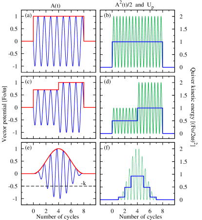
Figure 1: (Color online) Vector potential and quiver kinetic energy as function of the number of cycles $m=\omega t/2\pi$, for three envelopes: flat top, 1 step and sine squared envelope (top, middle and lower panels respectively). The laser pulse duration is equivalent to 8 cycles. Here $F_{1}=F_{0}/\sqrt{2}$, $F_{2}=F_{0}$ and $t_{1}=t_{2}=\tau/2$. Left column: Vector potential amplitude $A(t)$ in thin (blue) line and envelope of the laser field thick (red) line in units of $F_{0}/\omega$. Right column: quiver kinetic energy $A^{2}(t)/2$ in thin (green) line and cycle averaged quiver kinetic energy $U_{p}(m)$ in thick (blue) line in units of $(F_{0}/2\omega)^{2}$.

In order to illustrate the dependence of the ponderomotive energy with the envelope, let us consider a linearly polarized laser pulse modeled by the electric field

$$\mathbf{F}_{i}(t)=f_{i}(t)\,\cos{(\omega t)}\,\mathbf{\hat{\varepsilon}\,},$$ (16)

where we choose linear polarization along the direction $\hat{\varepsilon}$ and the total pulse duration $\tau=NT$ is such that the field oscillates $N$ cycles. We consider three different types of envelope $f_{i}(t)$ defined as

$$f_{1}(t) = F_{0}$$ (17)

$$f_{2}(t) = \begin{cases}F_{1},&\text{if }0<t<t_{1}\\ 0,&\text{if }t_{1}<t<t_{2}\\ F_{2},&\text{if }t_{2}<t<\tau\end{cases}$$ (18)

$$f_{3}(t) = F_{0}\,\sin^{2}(\pi t/\tau),$$ (19)

and zero outside the time interval $[0,\tau]$. Figure 1 presents the envelope, potential vector, quiver and ponderomotive energy for these three laser pulses for $N=8$. In the first case (Fig. 1(a) and (b)) corresponding to the flat top envelope, all cycles are identical to each other, the mean ponderomotive energy is equal to $(F_{0}/2\omega)^{2}$ along the pulse in a plane wave laser. Instead, the two step [$t_{1}=t_{2}$ in Eq. (18)] and sine squared [Eq. (19)] envelopes show clearly the dependence of $U_{p}$ on the $m$th cycle where the average is performed [see Fig. 1(d) and (f)]. However, to the best of our knowledge, for few-cycle laser pulses it is common to define in the literature a unique value of the ponderomotive energy as $U_{p}^{0}=(F_{0}/2\omega)^{2}$ with $F_{0}$ the maximal value of the envelope despite its strong envelope time variation.

Another important issue is about $\Delta\bm{\alpha}(m)$. As we have noted before, in the flat top [Eq. (17)] and step [Eq. (18)] cases, it is clear that $\Delta\bm{\alpha}(m)=0$ since the envelope remains constant during each cycle, whereas for the $f_{3}$ envelope it can be shown that $\Delta\bm{\alpha}(m)$ decreases as $N$ increases and it becomes negligible at the middle of the pulse ($m\sim\frac{N}{2}$) where the laser intensity (and then the probability of electronic emission in ionization problems) is maximum.

III Above threshold ionization

We consider the problem of above threshold ionization of one-electron atom due to the interaction with a classical EM field, in particular, short laser pulses. It is known that ATI peaks produced by long pulses in the PE spectra are located in the positions given by Eq. (1). Its validity requires an initial and final state energies well defined. However, when a laser pulse impinges on an atom, the electron leaves its stationary state and its energy level changes over time and the simple relationship given by Eq. (1) is not exact for this time-dependent process. A reasonable approximation can be achieved by averaging the main value of $H$ [Eq. (10)] over a pulse optical cycle. As we have already explained, this is exact for a monochromatic pulse with flat envelope and the pulse has an integer number of cycles. When the pulse envelope varies in time it is not clear the concept of energy conservation Eq. (1) and the ensuing exact position of ATI peaks. For this reason, we will analyze the electron emission spectra and the validity of Eq. (1) in cases where the envelope results on a varying ponderomotive energy. We examine ionization of a hydrogen atom from the $1s$ state by short laser pulses with frequency and amplitude parameters such that the value $(F_{0}/2\omega)^{2}$, as indicator of the ponderomotive energy, is comparable to the separation of ATI peaks, i.e. $\omega$ and, therefore, Eq. (1) results sensitive to variations of the ponderomotive energy.

To investigate the PE spectra, especially within approaches based on time dependent quantum theory, the Volkov sate given by Eq. (8) has been widely used to describe the emitted electron immersed in the laser field. For example the Strong Field Approximation (SFA) Keldysh:64 ; Faisal:73 ; Reiss:80 ; Milosevic:06 , the Coulomb-Volkov Approximation (CVA) Duchateau:02 ; Rodriguez:04 ; Arbo:08 ; Gravielle:12 ; DellaPicca:13 and the semiclassical application of the Simple Man’s Model (SCM) Arbo:10R ; Arbo:10 ; Arbo:14 employ the non-stationary Volkov state as final wavefunction. The use of length gauge for the perturbation potential, i.e. $\mathbf{r}\cdot\mathbf{F}(t)$, and the Volkov state Eq. (13) also guarantee the presence of $U_{p}$ in the “final energy”, as we have mentioned before.

Within the time-dependent distorted wave theory, the transition amplitude in the prior form and length gauge is expressed as

$$T_{if}=-i\int_{0}^{\tau}\big{\langle}\chi_{f}^{-}(\mathbf{r},t)|\mathbf{r}\cdot\mathbf{F}(t)|\Phi_{i}(\mathbf{r},t)\big{\rangle}\,\mathrm{d}t$$ (20)

where $\Phi_{i}(\mathbf{r},t)=\varphi(\mathbf{r})\,\mathrm{e}^{\mathrm{i}I_{p}t}$ is the $1s$ initial state of the hydrogen atom and $\chi_{f}^{-}(\mathbf{r},t)$ is the length Volkov state Eq. (13) in the SFA. In the CVA, $\chi_{f}^{-}$ includes the coulomb distortion as an additional factor:

$$\chi_{f}^{-}(\mathbf{r},t)=\chi^{L}(\mathbf{r},t)\,D_{C}^{-}(\mathbf{k},\mathbf{r})$$ (21)

where $D_{C}^{-}(\mathbf{k},\mathbf{r})=N(\nu)\,{{}_{1}F_{1}}\left(\mathrm{i}\nu;1;-\mathrm{i}(kr+\mathbf{k}\cdot\mathbf{r})\right)$, the normalization factor is defined as $N(\nu)=\Gamma(1-\mathrm{i}\nu)\mathrm{e}^{-\pi\nu/2}$ and $\nu=-1/k$ is the Sommerfeld parameter, and ${{}_{1}F_{1}}$ is the hypergeometric function.

The photoelectron momentum distributions is obtained from the transition matrix magnitude as

$$\frac{\mathrm{d}P}{\mathrm{d}\mathbf{k}}=|T_{if}|^{2}$$ (22)

and the PE spectrum, that is the differential ionization probability of emitting electron with energy $E=k^{2}/2$, is

$$\frac{\mathrm{d}P}{\mathrm{d}E}=\int k\,|T_{if}|^{2}\mathrm{d}\Omega_{k}.$$ (23)

The semiclassical model (SCM) described in previous works Arbo:10R ; Arbo:10 ; Arbo:14 , utilizes the saddle point approximation to replace the time integration in Eq. (20) by a sum over ionization or release times $t_{r}$ where the oscillating phase

$$S(t)=\int_{0}^{t}\left[\frac{(\mathbf{k}+\mathbf{A}(t^{\prime}))^{2}}{2}+I_{p}\right]\mathrm{d}t^{\prime}$$ (24)

is stationary and has null derivative. Here, $S$ represents the modified Volkov action in which the energy of the initial state is included. The SCM approximates the complex release times $t_{r}$ with the real solutions of

$$\mathbf{k}+\mathbf{A}(t_{r})=0\,,$$ (25)

assuming that the electron is emitted from the atom into the continuum at the release time $t_{r}$ with zero initial velocity.

III.1 Flat-top pulse

The coherent superposition of classical trajectories associated with release times $t_{r}^{i}$ $(i=1,2,\dots)$ gives rise to semiclassical interferences, provided they satisfy the condition given by Eq. (25) for reaching the same final momentum $\mathbf{k}$. For a flat-top pulse the transition matrix can be written as

$$T_{if}=G(\mathbf{k})\sum_{i=1}^{M}\exp{\left[\mathrm{i}S(t_{r}^{i})\right]}\,,$$ (26)

where $M$ is the number of classical trajectories reaching a given final momentum $\mathbf{k}$ and $G(\mathbf{k})$ is the ionization amplitude that is independent of the emission times.

For an $N$-cycle flat top pulse (envelope defined in Eq. (17) and Fig. 1 a) there are two time solutions of Eq. (25) for each cycle $m$: $t_{1}^{m}$ and $t_{2}^{m}$. Let us introduce the difference and the average of the action evaluated at these times:

$$\Delta S = S(t_{2}^{m})-S(t_{1}^{m})$$ (27)

$$\overline{S}_{m} = \frac{S(t_{2}^{m})+S(t_{1}^{m})}{2}=S_{0}+m\bar{S}$$ (28)

where $\Delta S$ is the accumulated action, independent of the cycle $m$ and $\overline{S}_{m}$ is the average action in the $m$-cycle that depends linearly with $m$, where $\bar{S}=\frac{2\pi}{\omega}\left(\frac{k^{2}}{2}+U_{p}+I_{p}\right)$ and $S_{0}=-\bar{S}/2-kF_{0}/\omega^{2}$. We can derive an analytical expression for the transition amplitude as Arbo:10R ; Arbo:10

$$T_{if}=2\,G(\mathbf{k})\,\cos{\left(\frac{\Delta{S}}{2}\right)}\,\frac{\sin(N\bar{S}/2)}{\sin({\bar{S}/2})}\,\mathrm{e}^{\mathrm{i}(S_{0}+\frac{N+1}{2}\bar{S})}\,,$$ (29)

When the square modulus of Eq. (29) is considered, the factor $\cos^{2}(\Delta{S}/2)$ represents the form factor (or structure factor) accounting for intracycle interference, since it arises from the pairs of classical trajectories born at different times separated by $\Delta t=t_{2}^{m}-t_{1}^{m}$ between them. On the other hand, the factor $\left[\sin(N\bar{S}/2)/\sin({\bar{S}/2})\right]^{2}$ is the responsible for the intercycle interference, resulting in the well-known ATI peaks. In fact, when $N\rightarrow\infty$ this factor become a sequence of delta functions situated at $E_{n}$ values given by Eq. (1).

III.2 Semiclassical model for interpulse interference

For a more clear and comprehensive analysis of how the shape of the pulse envelope affects the PE spectra we assume an $N$-cycle laser pulse modeled by the simple time-dependent envelope $f_{2}(t)$, defined by two flat-top pulses with different amplitudes (as in Fig. 1 c-d) and separated by a time interval $\Delta t=t_{2}-t_{1}$. This last condition allows us to see how the interference pattern depends on the temporal separation between pulses. We assume that the time gap of $\Delta t$ corresponds to $M=\Delta t/T$ cycles, with $T=2\pi/\omega$. The first pulse corresponds to a $N_{1}$-cycle flat-top pulse with a field strength $F_{1}$ and the second to a $N_{2}$-cycle flat-top pulse with a field strength $F_{2}$, where $N_{1}=t_{1}/T$, $N_{2}=(\tau-t_{2})/T$ and $N=N_{1}+N_{2}+M$.

Since the perturbation is decomposed in two temporal contributions, the ionization amplitude can be written as the sum of the ionization amplitudes corresponding to each component of the pulse $T_{if}=T_{1}+T_{2}$ and consequently, the momentum distribution reads:

$$\frac{\mathrm{d}P}{\mathrm{d}\mathbf{k}}=|T_{1}|^{2}+|T_{2}|^{2}+2\,|T_{1}||T_{2}|\cos{\Phi}$$ (30)

where each term $T_{i}$ (with $i=1,2$) can be expressed as in Eq. (29). Then, the first two terms correspond to the individual emission probabilities that have the typical structure of ATI peaks at electron energies following Eq. (1) with the corresponding ponderomotive energy values $U_{p1}=\left(F_{1}/2\omega\right)^{2}$ and $U_{p2}=\left(F_{2}/2\omega\right)^{2}$. The third term accounts for the interference between the two contributions that we call interpulse interference term. The phase $\Phi$ results

$$\Phi = \frac{N_{1}\pi}{\omega}\left(I_{p}+\frac{k^{2}}{2}+U_{p1}\right)+\frac{N_{2}\pi}{\omega}\left(I_{p}+\frac{k^{2}}{2}+U_{p2}\right)$$ (31)

$$+\Delta t\left(I_{p}+\frac{k^{2}}{2}\right)+\frac{k}{\omega^{2}}(F_{1}-F_{2})\,.$$

The emission probability will have maximum and minimum values when $\Phi=\ell\pi$. According whether $\ell$ is odd or even the interference will be destructive or constructive, respectively. In these cases the emission probability is

$$\frac{\mathrm{d}P}{\mathrm{d}\mathbf{k}}=\left(|T_{1}|+(-1)^{\ell}|T_{2}|\right)^{2}$$ (32)

This take place at $k_{\ell}$ values, that are solutions of the quadratic equation $\Phi=\ell\pi$, where $\Phi$ is given by Eq. (31). Let us consider the separation between two successive “interpulse interference-peaks” (even $\ell$) in the PE spectra. It is easy to see that

$$2\pi=(k_{\ell+2}^{2}-k_{\ell}^{2})\,\frac{\pi(N+M)}{2\omega}+(k_{\ell+2}-k_{\ell})\frac{(F_{1}-F_{2})}{\omega^{2}}$$ (33)

This pattern (a sequence of minima and maxima every time that the electron momentum verifies $\Phi=\ell\pi$) is superimposed to the sum of individual PE spectra originating from each pulse contribution. This interpulse interference pattern is observed as fine structure on each intercycle peak.

In particular, when we consider two identical steps ($F_{1}=F_{2}$ and $N_{1}=N_{2}$), the ionization probability in Eq. (30) reads

$$\frac{\mathrm{d}P}{\mathrm{d}\mathbf{k}}=4\,|T_{1}|^{2}\,\cos^{2}{(\Phi/2)}$$ (34)

and the phase is reduced to $\Phi=t_{2}\left(I_{p}+\frac{k^{2}}{2}\right)+t_{1}\,U_{p1}$, or what is the same $\Phi=t_{1}\left(I_{p}+\frac{k^{2}}{2}+U_{p1}\right)+\Delta t\left(I_{p}+\frac{k^{2}}{2}\right)$. In this situation, the interpulse interference is clearly marked as an oscillating modulation over the single PE spectrum and it becomes destructive or constructive according to the time delay between cycles.

III.3 Analysis of PE spectra produced by a few-step envelope pulse

In this section we evaluate the PE spectra for ionization of the hydrogen atom from the $1s$ state by laser pulses with envelope defined in Eq. (18), using the SCM approximation described above. This will give evidence of the interferences between cycles with different ponderomotive energy.

In Fig. 2 we present the PE spectra for $F_{1}=0.2$ a.u. and $F_{2}=0.2$ a.u. and $0.225$ a.u., in left and right column respectively and variable time delay $\Delta t$, while keeping the frequency constant $\omega=0.25$ a.u. and the number of cycles $N_{1}=N_{2}=8$. The rows of Fig. 2 correspond to different temporal delays between the two pulses. In the first row we show the PE spectra for the not delay ($t_{2}=t_{1}$) case. In (a), as there is no time delay, i.e., $\Delta t=0$ the two half pulses with amplitude $F_{1}=F_{2}=F_{0}$ merge in a flat top pulse [Fig. 1 (a)] and the ponderomotive energy can be uniquely defined as $U_{p}=U_{p}^{0}=(F_{0}/2\omega)^{2}$ [see Fig. 1 (b)] and the PE spectrum is equivalent to that obtained from a $N=16$ cycle laser pulse and the ATI peak observed corresponds to the absorption of $n=3$ photons in agreement with Eq. (1). In turn, when the two half pulses have different amplitudes [Fig. 2 (b)], we observe the presence of ATI peaks at electron energies (marked with vertical dashed lines) according to Eq. (1) with $U_{p1}=\left(F_{1}/2\omega\right)^{2}$ and $U_{p2}=\left(F_{2}/2\omega\right)^{2}$ values. The energy separation between the two peaks agrees with the prediction $\Delta E=U_{p2}-U_{p1}=(F_{2}^{2}-F_{1}^{2})/4\omega^{2}=0.0425$ a.u.. In Fig. 2 (b) we add with a thin (green) line the PE spectrum for the smaller pulse alone ($F_{1}=0.2$ a.u. and $F_{2}=0$). We observe that the presence of the field with amplitude $F_{2}$ not only produces an ATI peak at $E=0.09$ a.u, according to Eq. (1) with $U_{p2}=\left(F_{2}/2\omega\right)^{2}$, but also the interference structures at the main and lateral peaks in agreement with the theory of interpulse interference described in the last subsection.

When the interpulse delay increases (middle and lower rows) we observe a subtle oscillating structure due to the interpulse interference term: the energy separation between consecutive peaks decreases as increasing $M$ [Eq. (33)]. This oscillating pattern is maximum when amplitudes are equals (left column) and diminishes as the amplitude difference $|F_{2}-F_{1}|$ increases (right column). In the former the interference leads to a null emission probability at certain energy values following Eq. (34).

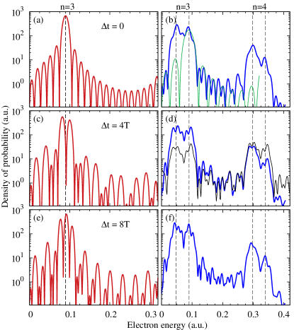
Figure 2: (Color online) H(1s) ATI PE spectra obtained within the SCM by laser pulses with envelope given by Eq. (18) with $\omega=0.25$ a.u., $N_{1}=N_{2}=8$ cycles and $F_{1}=0.2$ a.u.. Left column (red lines): two identical pulses case with $F_{1}=F_{2}$. Right column (blue lines): $F_{2}=0.225$ a.u.. Vertical dashed lines indicates the position of the ATI peaks following Eq. (1) with $U_{p1}$ and $U_{p2}$ values. The upper labels $n=3$ or $4$ indicate the number of absorbed photons. In (a-b), (c-d) and (e-f) cases the time delay between the two parts of the pulse are $0,4$ and $8$ cycles, respectively. In (b) PE spectrum for a flat top with 8 cycle pulse in thin (green) line. In (d) CVA PE spectrum with thin (black) line.

In order to check the validity of the employed model we compare the SCM and the CVA PE spectra in Fig 2 (d). We observe that despite SCM overestimates the emission probability, both calculations results in practically the same interference pattern.

Summarizing, from this simple example we can distinguish two different effects on the PE spectrum due to the time-dependent envelope: (i) different ATI peaks are expected at different energy positions depending on the field strengths, or what is the same, the emission time intervals, and (ii) different field strengths and the temporal delay provoke an interference pattern that is maximal when the pulses are identical affecting the shapes of the ATI peaks. The first conclusion (i) can be easily deduced from the individual contributions $|T_{i}|^{2}$ in Eq. (30), whereas the second (ii) has its origin in the interpulse interference term.

In the same way as the simple cases mentioned above, the ionization amplitudes for pulses with a several-step envelope could also be written as sum of contribution from each part of the pulse, and this leads to interferences in the emission probability. In this situation the number of interfering terms will be large, the associated peaks superpose and a possible recognition could be lost. However, the general analysis for the two step pulse can be easily extrapolated to several-step pulses and therefore, a more deep understanding of the shape of the spectra could be achieved.

In the Fig. 3 we show the PE spectra corresponding to a symmetric pulse with three different field amplitudes $0.8F_{0}$, $0.9F_{0}$ and $F_{0}$, as shown in the inset of figure 3 (a). Each step involves 8 cycles, $F_{0}=0.25$ a.u. and $\omega=0.25$ a.u.. As before, we can consider that this pulse is a superposition of several short pulses with different amplitudes. Therefore, the resulting electron emission probability results from the sum of 5 terms $|Ti|^{2}$ and 10 interference terms ($T_{i}T_{j}^{\ast}+T_{i}^{\ast}T_{j}$) with $1\leq i,j\leq 5$ and $i\neq j$. As before, the main contribution to the interference effects will come from the amplitudes corresponding to pair of steps with the same electric field amplitude, temporarily delayed. We evaluate independently each of these pair of steps and the results are displayed in Fig 3 (b). There we observe that the position of the ATI peaks are given by Eq. (1) with their respective ponderomotive energies, as it is indicated by the broken lines. A comparison of Fig 3 (a) with 3 (b) clearly shows that the contributions from the time delayed interference terms between $T_{1}$ and $T_{5}$ and between $T_{2}$ and $T_{4}$ dominate the respective ATI peaks. These interferences have an analytical representation as given by Eq. (34). Furthermore, we have checked that the ATI peak at $0.25$ a.u. due to the central highest step (red contribution in inset of Fig 3(b)) reproduces the non-symmetric shape that it acquires in Fig. 3(a) when the neighboring level of lower amplitude (blue contribution in inset of Fig 3(b)) is also considered (not shown). An important consequence of conclusion (i) is that we can consider that ATI peaks have a maximum spread directly related to the spread of the ponderomotive energy values. In the case of Fig 3 this means that the ATI peak for $n=4$ photon absorption is comprised in the electron energy range between $0.25$ to $0.34$ a.u.

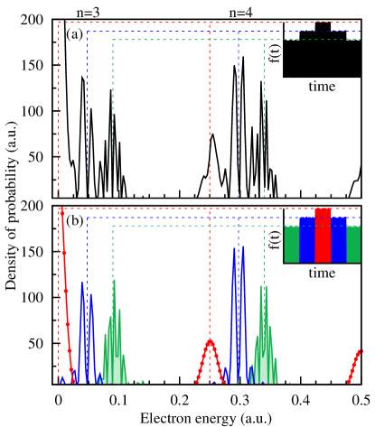
Figure 3: (Color online) CVA H(1s) ATI PE spectra with $F_{0}=\omega=0.25$ a.u. and envelope shown in the inset. (a) CVA PE spectrum for 5-level envelope. (b) PE spectra for one step of amplitude $F_{0}$ with (red) line with dots, for two step of amplitude $0.9F_{0}$ delayed 8 cycles with (blue) thick line and for two step of amplitude $0.8F_{0}$ delayed 24 cycles with (green) filled curve line.

III.4 The PE spectra for a continuous envelope

We consider an electric field with a more realistic envelope described by a continuous smooth envelope [Eq. (19)]. Following the SCM, electron trajectories released at different ionization times interfere producing an interference pattern. These ionization times can be easily calculated as $\mathbf{k}+\mathbf{A}(t_{r})=0$. Unlike the flat-top pulse, ionization times are not equally spaced in the continuous envelope case, i.e., sine-squared envelope (see Fig. 1(e)). The temporal separation of these slits depends on the electron energy and the particular envelope function. Only the cycles with sufficient intensity will significantly contribute to the electron emission with a given momenta $\mathbf{k}$. In other words, unlike Eq. (27) for a flat top pulses, the accumulated action $\Delta S$ does depend on each particular cycle. The action in Eq. (24) depends on the shape of the envelope and the number of cycles involved, and it does not scale linearly with the cycle order. Therefore, the intercycle interference will not be described by a simple periodic function as before and the electron spectra will not exhibit a homogeneous periodic interference pattern. Anyhow, we are able to analyze qualitatively the PE spectrum in view of the previous analysis.

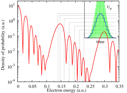
Figure 4: (Color online) H(1s) CVA ATI PE spectra for sinusoidal envelope with $F_{0}=0.1$ a.u., $\omega=0.15$ a.u. and $N=24$ cycles. In the inset we show the quiver (in thin green line) and the cycle dependent ponderomotive energy (in thick blue line) as function of time.

The electron emission will be maximum near the center of the pulse ($t\simeq\tau/2)$, that is for the strongest values of the field. Therefore, in the atomic process of absorption of $n$ photons, the kinetic energy will have an lower bound limit given by Eq. (1), with ponderomotive energy $U_{p}^{0}=(F_{0}/2\omega)^{2}$. The electrons emitted by lower field values in the pulse will feel a lower ponderomotive energy and therefore will acquire a higher kinetic energy with decreasing emission probability. In other words, the minimal strength electric field at the beginning and the end of the pulse produces negligible contribution to the PE spectrum at maximal value of the electron energy $E_{n}=n\omega-I_{p}$. In the middle between both situations, as the field envelope vary continuously the ponderomotive energy is strong dependent on the cycle $(t_{0},t_{0}+2\pi/\omega)$ where the quiver energy average is perform. Depending on the time $t_{0}$ we can expect continuous values of $U_{p}$ between $0$ and $U_{p}^{0}$ and therefore some structures in the PE spectrum are expected in the energy range $(n\omega-I_{p}-U_{p}^{0},n\omega-I_{p})$ where effect (ii) described in previous section, is also added. Then, the width of the energy range of each peak is the peak ponderomotive energy $U_{p}^{0}$, provided $U_{p}^{0}<\omega$, and therefore it is independent of the pulse duration. As an example, we display in Fig. 4 the CVA PE spectrum produced by a sinusoidal pulse with $\omega=0.15$ a.u., $F_{0}=0.10$ a.u. and $N=24$. There it can be observed that the ATI peak corresponding to $n=5$ absorbed photons starts at electron energy $5\omega-I_{p}-U_{p}^{0}=0.139$ a.u. (when the field is maximum) and finishes at $5\omega-I_{p}=0.25$ a.u.. In the inset of the figure, as in Fig. 1 (f), we show the cycle averages of the quiver energy, i.e. the ponderomotive energy, which are associated to the electron energies indicated by dashed lines in the main graph. In this case, they coincide whit the substructures peaks.

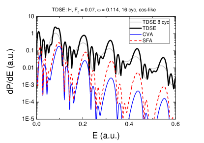
Figure 5: (Color online) H(1s) TDSE (black thick line), CVA (blue thin line), and SFA (red dashed line) PE spectra for sinusoidal envelope with $F_{0}=0.07$ a.u., $\omega=0.114$ a.u. and $N=16$ cycles.

These results are corroborated with the ab initio solution of the TDSE in the SAE approximation tong97 ; tong00 ; Arbo06prl . The existence of the shifted ATI peaks with different values of the ponderomotive energy appears also in the TDSE calculations (Fig. 5). The exact positions of the peaks do not exactly coincide with the CVA and SFA calculations, which happens to be slightly displaced to higher energies. The comparison between CVA and SFA PE spectra indicates that the effect of the long-range Coulomb potential, which is accounted approximately in CVA and neglected in SFA, does not have any significant effect in the formation of the substructure by a rapidly changing ponderomotive energy Wickenhauser:06 .

IV Conclusions

The quiver energy acquired by an atomic electron in a laser field is a time dependent quantity, that produces a strong time variation of the electron kinetic energy. For a simple interpretation of the emitted electron spectra it is usual to introduce the ponderomotive energy as the time average of the quiver energy, and use it in a stationary energy conservation rule. We show that this approximation is reasonable for pulses with flat envelopes, but it is poor for fast changing pulse envelopes. Firstly, we consider multiple-step pulses with an envelope that is constant in different regions of the time domain and show that each step of constant envelope leads to a peak in the PE spectra with position determined by Eq. (1) with the corresponding stepponderomotive energy $U_{p}$. We found that the electron emission amplitudes produced by the steps interfere with each other and produce a new pattern additional to the inter-cycle peaks. We derive an analytic expression for these interferences for the two step envelope and discuss how the PE spectrum varies as a function of the relative field strength and the time delay between steps. When the pulse has a non constant continuous envelope function the intensity of the electric field and ponderomotive energy changes concurrently. We found that the electron ionization energy spectra is characterized by well known ATI peaks with a width (or substructures) associated to the variation of ponderomotive energy values. Therefore, the shape of these peaks follows the shape of the envelope.

- [1] P. Agostini, F. Fabre, G. Mainfray, G. Petite, and N. K. Rahman. Free-free transitions following six-photon ionization of xenon atoms. Phys. Rev. Lett., 42:1127–1130, Apr 1979.
- [2] D. G. Arbó, S. Yoshida, E. Persson, K. I. Dimitriou, and J. Burgdörfer. Interference Oscillations in the Angular Distribution of Laser-Ionized Electrons near Ionization Threshold. Physical Review Letters, 96(14):143003, April 2006.
- [3] Diego G. Arbó, Kenichi L. Ishikawa, Klaus Schiessl, Emil Persson, and Joachim Burgdörfer. Diffraction at a time grating in above-threshold ionization: The influence of the coulomb potential. Phys. Rev. A, 82:043426, Oct 2010.
- [4] Diego G. Arbó, Kenichi L. Ishikawa, Klaus Schiessl, Emil Persson, and Joachim Burgdörfer. Intracycle and intercycle interferences in above-threshold ionization: The time grating. Phys. Rev. A, 81:021403, Feb 2010.
- [5] Diego G. Arbó, Jorge E. Miraglia, María Silvia Gravielle, Klaus Schiessl, Emil Persson, and Joachim Burgdörfer. Coulomb-volkov approximation for near-threshold ionization by short laser pulses. Phys. Rev. A, 77:013401, Jan 2008.
- [6] Diego G. Arbó, Stefan Nagele, Xiao-Min Tong, Xinhua Xie, Markus Kitzler, and Joachim Burgdörfer. Interference of electron wave packets in atomic ionization by subcycle sculpted laser pulses. Phys. Rev. A, 89:043414, Apr 2014.
- [7] C. C. Chirilă and R. M. Potvliege. Low-order above-threshold ionization in intense few-cycle laser pulses. Phys. Rev. A, 71:021402, Feb 2005.
- [8] R. Della Picca, J. Fiol, and P. D. Fainstein. Factorization of laser–pulse ionization probabilities in the multiphotonic regime. Journal of Physics B: Atomic, Molecular and Optical Physics, 46(17):175603, 2013.
- [9] Philipp V. Demekhin and Lorenz S. Cederbaum. Dynamic interference of photoelectrons produced by high-frequency laser pulses. Phys. Rev. Lett., 108:253001, Jun 2012.
- [10] L. F. Di Mauro and P. Agostini. Ionization dynamics in strong laser fields, Advances in Atomic, Molecular and Optical Physics, volume 35. Academic Press, 1995.
- [11] G. Duchateau, E. Cormier, and R. Gayet. Coulomb-volkov approach of ionization by extreme-ultraviolet laser pulses in the subfemtosecond regime. Phys. Rev. A, 66:023412, Aug 2002.
- [12] D B Miloěvić, G G Paulus, D Bauer, and W Becker. Above-threshold ionization by few-cycle pulses. Journal of Physics B: Atomic, Molecular and Optical Physics, 39(14):R203, 2006.
- [13] F H M Faisal. Multiple absorption of laser photons by atoms. Journal of Physics B: Atomic and Molecular Physics, 6(4):L89, 1973.
- [14] W. Gordon. Der comptoneffekt nach der schrödingerschen theorie. Zeitschrift für Physik, 40(1-2):117–133, 1926.
- [15] M S Gravielle, D G Arbó, J E Miraglia, and M F Ciappina. A doubly distorted-wave method for atomic ionization by ultrashort laser pulses. Journal of Physics B: Atomic, Molecular and Optical Physics, 45(1):015601, 2012.
- [16] C. J. Joachain, N. J. Kylstra, and R. M. Potvliege. Atoms in intense laser fields. Cambridge University Press, 2012. Chap. 2.
- [17] L. V. Keldysh. Zh. Eksp. Teor. Fiz., 47:1945, 1964.
- [18] M. Lewenstein, Ph. Balcou, M. Yu. Ivanov, Anne L’Huillier, and P. B. Corkum. Theory of high-harmonic generation by low-frequency laser fields. Phys. Rev. A, 49:2117–2132, Mar 1994.
- [19] M. Lewenstein, K. C. Kulander, K. J. Schafer, and P. H. Bucksbaum. Rings in above-threshold ionization: A quasiclassical analysis. Phys. Rev. A, 51:1495–1507, Feb 1995.
- [20] F. Lindner, M. G. Schätzel, H. Walther, A. Baltuška, E. Goulielmakis, F. Krausz, D. B. Milošević, D. Bauer, W. Becker, and G. G. Paulus. Attosecond double-slit experiment. Phys. Rev. Lett., 95:040401, Jul 2005.
- [21] Jonathan Parker and Charles W. Clark. Study of a plane-wave final-state theory of above-threshold ionization and harmonic generation. J. Opt. Soc. Am. B, 13(2):371–379, Feb 1996.
- [22] Howard R. Reiss. Effect of an intense electromagnetic field on a weakly bound system. Phys. Rev. A, 22:1786–1813, Nov 1980.
- [23] V. D. Rodríguez, E. Cormier, and R. Gayet. Ionization by short uv laser pulses: Secondary above-threshold-ionization peaks of the electron spectrum investigated through a modified coulomb-volkov approach. Phys. Rev. A, 69:053402, May 2004.
- [24] X.-M. Tong and S.-I. Chu. Theoretical study of multiple high-order harmonic generation by intense ultrashort pulsed laser fields: A new generalized pseudospectral time-dependent method. Chemical Physics, 217:119–130, May 1997.
- [25] X.-M. Tong and S.-I. Chu. Probing the spectral and temporal structures of high-order harmonic generation in intense laser pulses. Phys. Rev. A, 61(2):021802, February 2000.
- [26] M. Wickenhauser, X. M. Tong, and C. D. Lin. Laser-induced substructures in above-threshold-ionization spectra from intense few-cycle laser pulses. Phys. Rev. A, 73:011401, Jan 2006.
- [27] D.M. Wolkow. Über eine klasse von lösungen der diracschen gleichung. Zeitschrift für Physik, 94(3-4):250–260, 1935.